Not show value excel - Word и Excel - помощь в работе с программами

Excel for Microsoft 365 Excel 2021 Excel 2019 Excel 2016 Excel 2013 Excel 2010 Excel 2007 More…Less

Suppose you have a worksheet that contains confidential information, such as employee salaries, that you do not want a co-worker who stops by your desk to see. Or perhaps you multiply the values in a range of cells by the value in another cell that you do not want to be visible on the worksheet. By applying a custom number format, you can hide the values of those cells on the worksheet.

Note: Although cells with hidden values appear blank on the worksheet, their values remain displayed in the formula bar where you can work with them.

Hide cell values

Select the cell or range of cells that contains values that you want to hide. For more information, see Select cells, ranges, rows, or columns on a worksheet .

Note: The selected cells will appear blank on the worksheet, but a value appears in the formula bar when you click one of the cells.
On the Home tab, click the Dialog Box Launcher next to Number.
In the Category box, click Custom.
In the Type box, select the existing codes.
Type ;;; (three semicolons).
Click OK.

Tip: To cancel a selection of cells, click any cell on the worksheet.

Display hidden cell values

Select the cell or range of cells that contains values that are hidden. For more information, see Select cells, ranges, rows, or columns on a worksheet .
On the Home tab, click the Dialog Box Launcher next to Number.
In the Category box, click General to apply the default number format, or click the date, time, or number format that you want.

Tip: To cancel a selection of cells, click any cell on the worksheet.

Need more help?

Источник

Sometimes, when you open an Excel spreadsheet, you can’t see the text you have typed in a cell.

The text may be visible on the formula bar but not in the cell itself. For instance, in the image below, the data in cell C2 is not visible but you can see it in the formula bar.

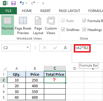
Figure 1 — Excel Not Showing Data in Cells

Also Read: Data Disappears in Excel – How to Get it Back?

Workarounds to Fix ‘Excel Not Showing Data in Cells’

Note: Before trying these workarounds, make sure that your Office program is updated.

Workaround 1 – Check for Hidden Cell Values

If cell values are hidden, you won’t be able to see data when a cell is selected. But the data will be visible in the formula bar. To display hidden cell values in a worksheet, follow these steps:

Select a single cell or range of cells that doesn’t show the text.
Right-click on the selected cell or range of cells and choose Format Cells.

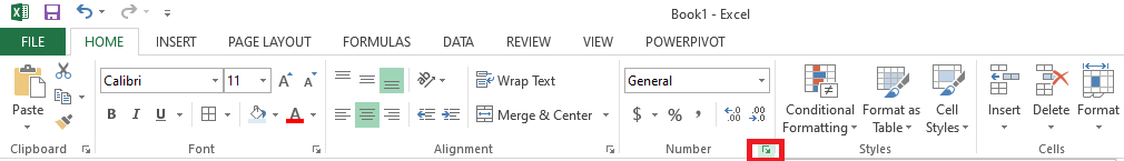
Figure 2 — Select Format Cells

A ‘Format Cells’ window opens. On the Number tab, choose Custom and check if 3 semi-colons (;;;) appear in the Type textbox.

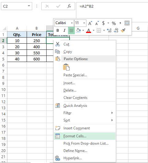
Figure 3 — Check for Semi-Colons in Type Box

If you can see the 3 semi-colons, delete them and then click OK. If you cannot see semi-colons in the ‘Type’ textbox, skip to the next workaround.

Workaround 2 – Change the Default Font

The font of cells in your Excel worksheet may be creating the problem. So, try changing the default font of cells or ranges:

Select a cell or cell range where the text is not showing up.
Right-click on the selected cell or cell range and click Format Cells.
From the pop-up window, click on the Font tab and then change the default font (usually Calibri) to any other font, like ‘Arial’ or ‘Times New Roman’. Press the OK button.

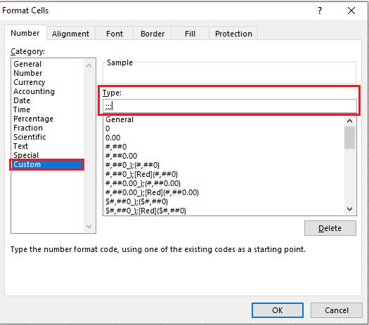
Figure 4 – Format Cells Window

If changing the default font doesn’t fix the ‘Excel data not showing in cell’ problem, proceed with the next workaround.

Workaround 3 – Disable Allow Editing Directly in Cell Option

Some users have reported that they were able to resolve the ‘Excel data not showing in cells’ issue by unchecking the ‘Allow editing directly in cells’ option. To do so, follow these steps:

In Excel, click on the File menu and then click on Options.

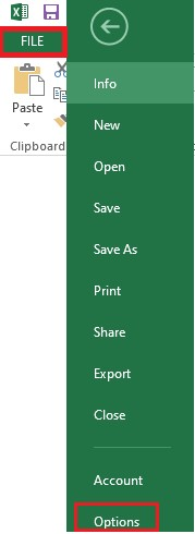
Figure 5 — Excel Options

From the Excel Options window, choose Advanced in the left pane and then uncheck ‘Allow editing directly in cells’.

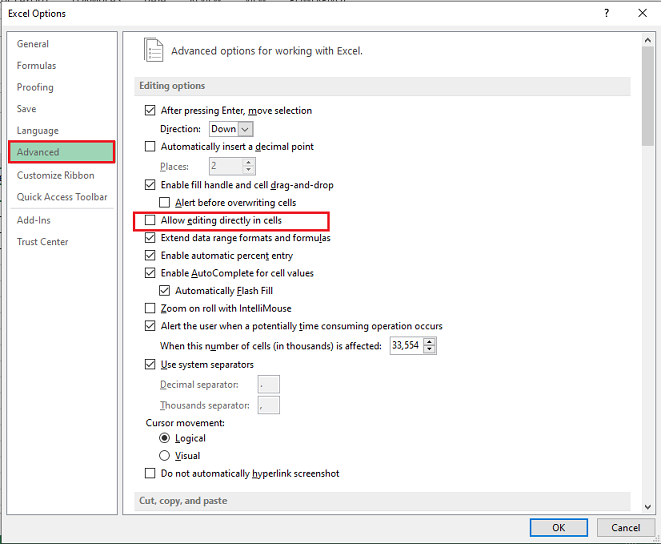
Figure 6 — Uncheck Allow Editing Directly in Cells

Click OK.

If you are unable to view the text in Excel cells, try the next workaround.

Workaround 4 – Adjust Row Height to Make the Cell Data Visible

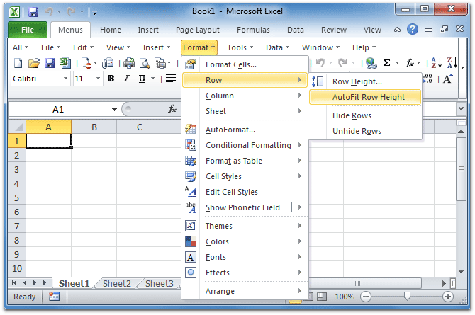
If you have cells with wrapped text, then try adjusting the row height of the cell or range to make the data visible. Here are the steps:

Select a specific cell or range for adjusting the row height.
On the Home tab, click Format from the Cells group.

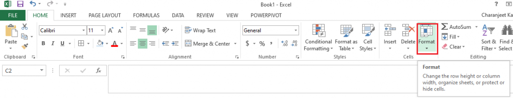
Figure 7 — Format Option in Cells Group

Under Cell Size, perform any of these actions:
Click AutoFit Row Height to automatically adjust the row height of your cell or cell range.
Click Row Height to manually enter a cell’s row height. This will open a ‘Row Height’ box. In the box, enter the row height that you want.

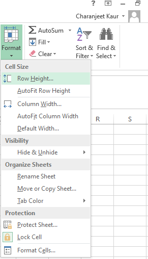
Figure 8 – Cell Size Options

Tip: You can also adjust a cell’s row height by dragging the bottom border of the row till the height when the wrapped text is visible.

Workaround 5 – Recover Missing Cell Content

Your Excel worksheet won’t display data in cells if it is corrupted. In other words, the cell values won’t display any result if the data in your Excel worksheet is damaged or corrupted. In that case, you can manually fix and recover corrupt Excel files or use an Excel repair tool, such as Stellar Repair for Excel.

Read this: How to Recover Corrupted Excel File?

Using the Excel file repair tool can help you retrieve all your worksheet data, including cell content, tables, numbers, text, rules, etc.

Wrapping Up

Oftentimes, when opening an Excel worksheet or while working on one, clicking on a cell or cell range doesn’t show any data. You may be able to see the data in the formula bar of your worksheet but not within the cells. This may prevent you from doing anything constructive in Excel. Try troubleshooting the issue by using the workarounds discussed in this article. If nothing works, chances are that corruption in the Excel file is causing it to behave oddly. Try repairing corrupt Excel file by using the built-in ‘Open and Repair’ feature or use Excel file repair software by Stellar to quickly restore your worksheet with all its data intact.

You might also be interested in reading:

[Fix] Excel formula not showing result

Easy Steps to Make Excel Hyperlinks Working

Источник

Does your Excel cell content not visible but show in formula bar? Don’t have any idea why is the text not showing in Excel cells?

Want to know how you can solve this Excel text disappears in cell mystery?

In that case, this particular post is very important to read. As it contains complete detail on how to fix Excel cell contents not visible issues.

User’s Query:

Let’s understand this issue more clearly with these user complaints.

Issue: Content of Excel cells invisible while typing

If I’m typing text or numbers into an Excel cell, while I can see what I’m writing in the formula bar above the chart, the cell shows nothing but the vertical stroke of a cursor, and no text or numbers at all until I tab out of the cell. I find this very annoying, though not a stopper to doing work. It’s unlike any Excel I’ve used in the past.

Source: https://answers.microsoft.com/en-us/msoffice/forum/all/content-of-excel-cells-invisible-while-typing/7937a331-4b27-4790-adda-9341d2010f10?auth=1

To recover lost Excel cell contents, we recommend this tool:

This software will prevent Excel workbook data such as BI data, financial reports & other analytical information from corruption and data loss. With this software you can rebuild corrupt Excel files and restore every single visual representation & dataset to its original, intact state in 3 easy steps:

Download Excel File Repair Tool rated Excellent by Softpedia, Softonic & CNET.
Select the corrupt Excel file (XLS, XLSX) & click Repair to initiate the repair process.
Preview the repaired files and click Save File to save the files at desired location.

These are the fixes that you all must try to get rid of the issue Excel cell contents not visible but show in formula bar.

1# Set The Cell Format To Text
2# Display Hidden Excel Cell Values
3# Using The Autofit Column Width Function
4# Display Cell Contents With Wrap Text Function
5# Adjust Row Height For Cell Content Visibility
6# Reposition Cell Content By Modifying The Alignment Or Rotating Text
7# Retrieve Missing Excel Cell Content

Let’s discuss all these fixes in detail….!

Fix 1# Set The Cell Format To Text

If you are facing this Excel cell contents not visible issue with a particular formula. Even after checking the formula, you haven’t found any error but still, it not showing the result.

In that case, immediately check whether the cell format is set to text or not.
You can also set the format of the cell to another suitable number format.
Now you need to get into the “cell edit mode” so that Excel can easily identify the format modification. For this just make a tap on the formula bar and hit enter.

Fix 2# Display Hidden Excel Cell Values

Choose either the range of the cell or the cells having hidden values.

Tip: you can easily cancel the cell selection, by tapping any cell present on the Excel worksheet.

Go to the Home tab and hit the Dialog Box Launcher which is present next to the Number.

Now from the Category box, tap to the General for application of the default number format.

Just tap on the number, date, or time, a format that you require.

Fix 3 # Using The Autofit Column Width Function

To display all the text not showing in Excel cell you can use the function Autofit Column Width.

It’s a very helpful feature to make easy adjustments in the column width of the cells. So this feature will, ultimately going to help in displaying all the hidden Excel cells content.

Here are the steps which you need to perform.

Choose the cell having hidden excel cell content and follow this path Home> Format > AutoFit Column Width.

After this, you will see all the cells of your worksheet will adjust their respective column width. This ultimately shows all the hidden Excel cell text.

Fix 4# Display Cell Contents With Wrap Text Function

With the Excel wrap text feature you can apply such cell formatting in which text will get wrap automatically or put a line break. After using the wrap text function your hidden excel cell content will start appearing in multiple lines.

Choose that cell whose content is not visible and tap to the Home> Wrap Text

After that, you will see your selected cell will be expanded with all the hidden content. Like this:

Note:

If still your Excel cell content not visible completely then maybe it’s because of the row size which is set to some specific height.

So follow the next solution of changing the row height to perfect content visibility.

Fix 5# Adjust Row Height For Cell Content Visibility

You can choose single or multiple rows in which you want to make a row height changes.
Go to the Home tab. Now from the Cells group choose the Format option.
Within the Cell Size, tap to the AutoFit Row Height.

Note: for quick autofit row height of the entire worksheet cells. Just tap to the Select All button. After that make double-tap on the boundary present just below the row heading.

Fix 6# Reposition Cell Content By Modifying The Alignment Or Rotating Text

For the perfect display of data in the worksheet, you must try repositioning the text present within the cell. For this, you can make modifications in the alignment of the cell content or you can use the indentation for correct spacing. Or else display the cell content at various angles by rotating it.

1. Select the range of the cells having the data which you wish to reposition.

2. Now make a right-click over the selected rows, you will get a list of options. From which you have to choose format cells.

3. In the opened dialog box of Format Cells choose the Alignment tab and perform any of the following operations:

Change the horizontal alignment of the cell contents
Change the vertical alignment of the cell contents
Indent the cell contents
Display the cell contents vertically from top to bottom
Rotate the text in a cell
Restore the default alignment of selected cells

Fix 7# Retrieve Missing Excel Cell Content

Another very high possibility of having this Excel cell content not visible issue is worksheet corruption. As it is found that data from Excel sheet goes missing when Excel file or worksheet got corrupted.

So either you can try the manual fixes to recover corrupt Excel file data. Or else go with experts recommended solution for recovery i.e Excel repair software.

Have a look over some catchy features of this software:

This supports the entire Excel version and the demo version is free.
This is a unique tool to repair multiple Excel files at one repair cycle and recovers the entire data in a preferred location.
This is unique software to repair multiple files at once and recover everything in the preferred location.
It is easy to use and compatible with both Windows as well as Mac operating systems.
With the help of this, you can fix all sorts of issues, corruption, errors in Excel workbooks.

Wrap Up:

By trying the above-mentioned fixes you can easily fix Excel cell contents not visible but show in formula bar issue. But even if the fixes fail to display hidden Excel cell content then immediately approach the software solution.

Don’t do unnecessary delay as this will lessen the possibility of complete Excel worksheet data recovery.

Priyanka is an entrepreneur & content marketing expert. She writes tech blogs and has expertise in MS Office, Excel, and other tech subjects. Her distinctive art of presenting tech information in the easy-to-understand language is very impressive. When not writing, she loves unplanned travels.

Источник

I’m working on an excel sheet and I’ve encountered an issue I’ve never come across before. I’m trying to sum the results of an array function, but I’m not getting any results from the sum on the sheet — just blank cells. The weird part is when I press F9 in the formula bar it shows the correct summed value that should show in the cells on the sheet. I just don’t get why the value would appear in the formula bar, but not in the cells on the sheet. Other forums mentioned changing the calculation option (on automatic of course) or to ‘show zeros’, which just changed the cells to zero instead of blank. F9 still shows the correct value. Here’s the formula:

{=SUM(OFFSET(INDIRECT("Sheet1!E"&IF(ISERROR(MATCH($A$2:$A$15&$C$1,Sheet1!$C$2:$C$51,0)),
1000,MATCH($A$2:$A$15&$C$1,Sheet1!$C$2:$C$51,0))),0,ROW(1:1)))}

The match gets me the row index for the numbers I need to sum. (E1000 is just a default for when there isn’t a match and references a cell with 0 in it). If I remove the sum from the function and use F9 I can see the actual array with the numbers to be summed. This is what is so confusing to me. Everything seems to evaluate correctly, it just doesn’t show on the sheet. Thanks for the help!

Xavier Guihot

52.1k21 gold badges284 silver badges183 bronze badges

asked Apr 28, 2016 at 7:29

I know this thread is a couple months old, but for anyone having this issue, try checking for Circular References. It is likely that your formula has at least one.

To check: click the Formulas tab, click the arrow next to Error Checking, point to Circular References, and then click the first cell listed in the submenu.

Reasoning: When using the Evaluate Formula function (F9), it only does a one time calculation and is able to give a complete result. However, if a circular reference is present, the formula in the sheet itself will continuously recalculate so may never have a definitive result.

answered Dec 11, 2016 at 19:33

I came here because I had the same issue, and the above did not initially work for me.

I found that to execute the array function you must highlight the entire formula and then (for Mac) press Control+Shift+Enter.

Once I did this it worked like a charm!!

Xavier Guihot

52.1k21 gold badges284 silver badges183 bronze badges

answered Mar 15, 2018 at 3:31

Joann Joann

111 bronze badge

Try «Recalculate All» on the formulas tab.

This solved a similar issue for me with an AVERAGEIF function, whose value would show up correctly in the formula viewer, but not in the sheet. Forcing the sheet to recalculate everything fixed the problem in my case.

The problem seems to occur when defining a cell that is based on another cell, that is based on other cells, that are based on other cells, that are based on other cells…at some point Excel seems to give up and assume that there’s a circular reference somewhere, even though there isn’t in my case.

When Excel calculates all sheets, it re-uses results, and ignores cells until their precedents are known, rather than working backward from a particular cell, so it doesn’t freak out if a cell relies on too many preceding cells.

answered Sep 7, 2018 at 3:59

Theodore MurdockTheodore Murdock

1,5181 gold badge13 silver badges27 bronze badges

Having the same problem, very frustrating. I have found an insane solution. I don’t know why it works but it does… I thought that I would try the formula in another cell. So I copied and pasted the cell in another cell… And the formula in the original cell worked and the correct value appeared.

answered Jul 5, 2016 at 0:28

I came across this problem when using SUMIFS with three queries on an array. I found the solution was to encapsulate the whole function in brackets. I think the problem must arise from the order in which excel evaluates the constituents of the formula when it derives its answer.

So for example I had to add the following brackets [highlighted in bold] =

SUMIFS( [00_COMBINED_NO_DUPLICATES.xlsx]COMBINED!$CK$2:$CK$60067,
        [00_COMBINED_NO_DUPLICATES.xlsx]COMBINED!$F$2:$F$60067,
        [@RR1],
        [00_COMBINED_NO_DUPLICATES.xlsx]COMBINED!$S$2:$S$60067,
        ">="&[@[Quarter_Starting]],
        [00_COMBINED_NO_DUPLICATES.xlsx]COMBINED!$S$2:$S$60067,
        "<"&EOMONTH([@[Quarter_Starting]],
        2
      )+1)

ρяσѕρєя K

132k52 gold badges197 silver badges213 bronze badges

answered Feb 1, 2017 at 0:20

AkanniAkanni

9249 silver badges10 bronze badges

This was happening to me. I solved it by pressing Ctrl and ‘
OR you can go to View, and unselect Show formulas.

In ‘normal’ Excel Ctrl+’ would insert the data from the cell above.

Hope this helps someone.

answered May 8, 2017 at 13:21

Make Calculate option as automatic. It should solve the probelem
See the screen shot

answered Jun 13, 2017 at 9:29

Sorry to reopen this but here is a new solution.

I do have circular references, deliberately, so I set Excel to allow them to evaluate only once. Default is OFF — do not evaluate, hence why your formulae returned false / 0 every time even if they appeared true.

To switch on Iterative calculations (i.e. do something with circular references instead of nothing): File -> Options -> Formulas -> Enable Iterative Calculations -> Change from 100 (a little excessive except in special applications) to 1.

Link (scroll down to the bit about iterative calculations): https://support.office.com/en-ie/article/remove-or-allow-a-circular-reference-8540bd0f-6e97-4483-bcf7-1b49cd50d123

Hope this helps some more folks!

answered Mar 27, 2019 at 12:34

jfgoodhew1jfgoodhew1

952 silver badges11 bronze badges

Sometimes it is a problem if you are using arrays with OFFSET or INDIRECT.
You can solve it using =N(INDIRECT(… or =N(OFFSET(

You can find the explanation below

Array Formula Confusion

answered Jun 22, 2020 at 18:56

Many of us have old ways to correct the formula, but let me tell you something: The iterative formula which shows correct results using «F9» means that you do not have to check the formula again and again.

You also do not have to check except the type=»general» — that’s it.

Now please please, please allow FILE>OPTIONS>FORMULAS>ENABLE ITERATIVE CALCULATION, maximum iteration = 300 (assuming you have 300 cells for iteration), maximum change = 0.001.

This is because we have to check whether the iteration is allowed or not. Hope your problem gets solved.

ouflak

2,44810 gold badges44 silver badges49 bronze badges

answered Oct 30, 2021 at 17:47

This problem also occurred when using an excel table reference. Converting the table to normal cells fixed it. Alternatively, changing the references from table to normal references fixed it too.

This part of a formula caused a #value / #wert error

VERGLEICH(LF5;DATWERT('Inzidenz RKI_20211129.xlsx'!Table6[[#Kopfzeilen];[27.09.2021]:[26.11.2021]]);0)

This did not:

VERGLEICH(LF5;DATWERT('[Inzidenz RKI_20211129.xlsx]LK_7-Tage-Fallzahl-aktualisiert'!$C$3:$C$173);0)

(vergleich is match, and datwert is datevalue in german excel, and it uses ; instead of commas)

answered Nov 29, 2021 at 7:08

DrWhatDrWhat

2,3305 gold badges19 silver badges31 bronze badges

Источник

This article is all about the #VALUE! error in Excel and the different ways to fix it. We will also look at the reasons why we encounter a #VALUE! in Excel in this tutorial.

What is #VALUE! error?

A #VALUE! error is displayed in an Excel spreadsheet when a value or formula is not the expected type. You are seeing this error probably because you entered a text value instead of a number value in a formula or a number value for a date value in a formula.

When does the #VALUE! error occur?

The #VALUE! error occurs due to multiple causes. Let us look at the different instances when this occurs in Excel.

1. Summing text and numerical values together

You can see that a series of cells that include text, date, and numerical values were summed up manually in the cell below. On pressing ENTER on the keyboard, the #VALUE! error shows up.

This happens because Excel is looking for a set of numerical or date values only to add them together and give an answer based on that. Excel is unable to add the values together because of a text value in between.

Note that no #VALUE! error is displayed when you sum these values using the SUM function in Excel. The SUM function is smarter and automatically removes all text values in the calculation.

2. Summing text values

In the image above, we have summed up three text values in three different cells together. Again, we didn’t use the SUM function here, and instead, we summed each value manually putting a + sign in the middle. As a result, we see a #VALUE! error.

The reason is simple. Excel cannot sum text values together. If you had used the SUM function to sum these text values together, the result would be 0 because it didn’t find any summable values in any cell.

The result will be the same if you try to find the difference between these values and almost any mathematical function in Excel.

3. Multiplying numbers with text or blank cells

In this image above, we are trying to multiply a text value with a number and the result is a #VALUE! error on pressing ENTER. Similarly, if you try to multiply a number with a blank cell in Excel you get the #VALUE! error.

A blank cell denotes a cell with an unnecessary space in an empty cell. A space in between formulas also gives a #VALUE! error in Excel.

4. Summing and multiplying ranges

In this image, we are trying to sum and multiply the two ranges but we get the result as a #VALUE! error. The reason is that the SUM function cannot add and multiply two ranges at a time. You need to use the SUMPRODUCT formula for that.

The SUMPRODUCT formula multiplies the adjacent values of corresponding ranges and returns a sum of it. However, the trick is to make the SUM formula work without having to use the SUMPRODUCT function is to press CTRL+SHIFT+ENTER before finishing the formula.

5. Providing a text value to the NETWORKDAYS function

The NETWORKDAYS function is used to count the working days between two dates. In the example above, we have provided a text value with a date value for the function that is unable to count the days and is giving the result as a #VALUE! error.

6. Creating an illogical IF formula

You can see that we did not provide any appropriate logical text for the IF formula to give an appropriate true or false value. You see a #VALUE! error displaying on pressing ENTER.

Tips to fix the #VALUE! error for different cases

Here are the tips to fix #VALUE! error in Excel for different instances like these.

1. Summing text and numerical values together

When you sum numbers manually without using the SUM function, make sure to add numbers with numbers or date values only based on your preferences and date values with date values only to avoid getting the #VALUE! error.

2. Summing only text values

Excel cannot add or subtract text values and will display the #VALUE error when you sum, multiply or subtract them manually. However, to avoid getting the error, use built-in formulas like SUM, PRODUCT, SUMPRODUCT, etc. to let Excel ignore a text or any other values that cannot be quantified.

3. Multiplying numbers with text or blank cells

If you have a blank space in a cell where you are applying a formula that is showing a #VALUE! error. Make sure to remove all unnecessary spaces from cells while you are applying a formula to a set of values.

If the dataset is too large to be modified, consider using the TRIM function on your datasets to remove all extra spaces and mistakes from them.

4. Summing and multiplying ranges

You cannot normally sum and multiply two ranges using the SUM formula in Excel. To be able to sum and multiple ranges at the same time, you can use the SUMPRODUCT function to multiply the corresponding ranges and give a sum of them.

Or, press CTRL+SHIFT+ENTER before finishing the SUM formula to make it work like the SUMPRODUCT formula.

5. Providing a text value to the NETWORKDAYS function

The NETWORKDAYS function requires two date values to count the number of working days between them. Avoid entering text or numerical values and end getting a vague answer or the famous #VALUE error.

6. Creating an illogical IF formula

Make sure you provide the IF function with an appropriate logical test. Here’s is an example of a correct IF function.

Here, we are creating a condition that if the values in the range are less than 20, then display “Low” in the active cell, if not, display “High” in the active cell.

Note that we have changed the values to help you understand how an IF function works.

Read more about the IF function in detail here.

Conclusion

This article was all about the #VALUE! error in Excel and the different ways to fix it. Stay tuned for more amazing Excel tutorials like this only on QuickExcel!

References: ExcelJet.

Источник