
Excel for Microsoft 365 for Mac Excel 2021 for Mac Excel 2019 for Mac Excel 2016 for Mac Excel for Mac 2011 More…Less
In Excel, the number that appears in a cell is separate from the number that is stored in the cell. For example, a number with seven decimal places may display as rounded when the cell format is set to display only two decimal places, or when the column isn’t wide enough to display the actual number. When performing a calculation, Excel uses the stored value, not the value that is visible in the cell.
To stop numbers from being displayed as rounded, you can increase the number of decimal places for that number, or you can increase the column width.
Note: By default, Excel displays two decimal places when you apply the number, currency, accounting, percentage, or scientific format to cells or data. You can specify the number of decimal places that you want to use when you apply these formats.
-
Select the column or columns that you want to change.
-
On the Format menu, point to Column, and then click AutoFit Selection.
Tips:
-
You can double-click a boundary to the right of one of the column headings to have the columns resize automatically.
-
To change the column width to a custom size, drag the boundary to the right of one of the column headings until the column is the size that you want.

-
-
Select the cell or range of cells that contains the numbers for which you want to increase the decimal places.
-
Do one of the following:
Excel 2016 for Mac: Click the Home tab, and then click Increase Decimal
once for each decimal place that you want to add.Excel for Mac 2011: On the Home tab, under Number, click Increase Decimal
once for each decimal place that you want to add.
 once for each decimal place that you want to add.
-
On the Format menu, click Cells, and then click the Number tab.
-
In the Category list, click Number, Currency, Accounting, Percentage, or Scientific depending on your cell data.
-
In the Decimal places box, enter the number of decimal places that you want to display.
See Also
Round a number to the decimal places I want
Need more help?
Want more options?
Explore subscription benefits, browse training courses, learn how to secure your device, and more.
Communities help you ask and answer questions, give feedback, and hear from experts with rich knowledge.
Isn’t it annoying when Excel just keeps rounding off numbers? Below table shows some common examples:
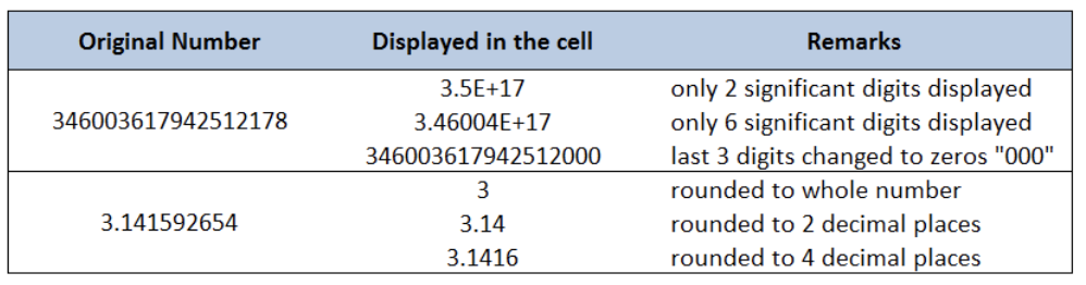 Figure 1. Examples of Excel Rounding Off Numbers
There are several possible reasons but the most common are these:
- Column width too narrow and doesn’t display the whole number
- The number of decimal places is set to fewer digits than the actual decimal places
- The number is too large and exceeds 15 digits; Excel is limited to display only 15 significant digits
- The default format for every cell in Excel is set to “General” and not “Number”
In this article we will discuss the following:
- Stop Excel From Rounding Large Numbers
- Stop Excel From Rounding Whole Numbers
- Stop Excel From Rounding Currency
Stop Excel From Rounding Large Numbers
There are instances when we need to enter large numbers, such as credit card or reference numbers. Unfortunately, Excel has a limitation and displays only 15 significant digits. The excess digits will be changed to zeros.
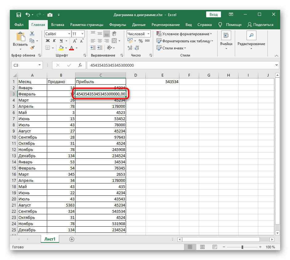
Example: In cell D3, enter the number “346003617942512178”, which contains 18 digits.
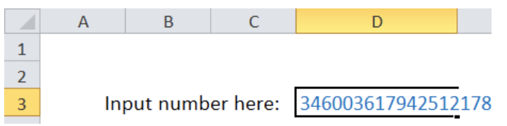 Figure 2. Entering an 18-digit number in Excel
Press enter. Cell D2 will display the value “3.46004E+17” while the formula bar will display the value “346003617942512000”.
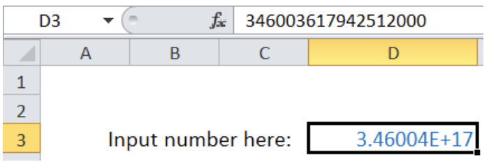 Figure 3. Excel rounding a large number and showing 15 significant digits only
Notes:
- The 16th to 18th digits are changed from “178” to “000”.
- The displayed value only shows 6 significant digits because default format in Excel is “General”
- To display the 18-digit number 346003617942512000, select D3 and press Ctrl + 1 to launch the Format Cells dialog box. Select the format “Number” and set the decimal places to zero “0”. The 18-digit number is now displayed in D3.
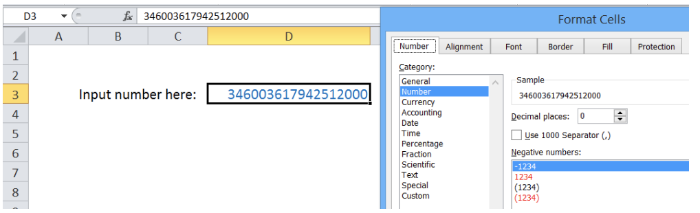 Figure 4. Changing the cell format from “General” to “Number”
But how to display the original number 346003617942512178?
Work-around:
To stop Excel from rounding a large number, especially those exceeding 15 digits, we can:
- Format the cell as text before entering the number; or
- Enter the number as a text by entering an apostrophe “ ‘ ” before the number
- Example: Enter into cell D3: ‘346003617942512178
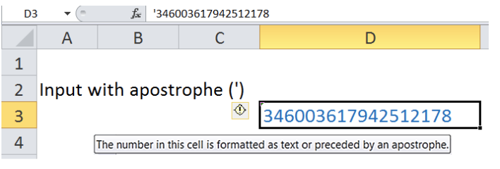 Figure 5. Entering the large number as text by preceding with an apostrophe
Stop Excel From Rounding Whole Numbers
Let’s take for example the value of pi(), which is commonly used in mathematical equations.
Example 1 : In cell D3, enter the formula =pi(). Column E displays the value of pi with varying number of decimal places.
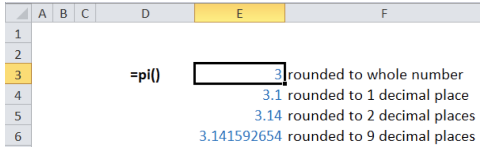 Figure 6. The value of pi() displayed with varying number of decimal places
Work-around:
To stop Excel from rounding whole numbers, click the Increase Decimal button in the Home > Number tab. Increase the decimal place until the desired number of decimal places is displayed.
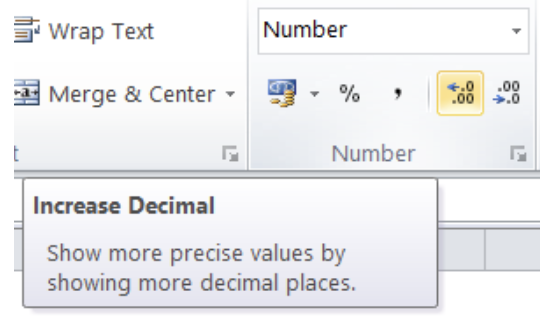 Figure 7. Increase Decimal button in Excel
Example 2: In cell D3, enter the number 123456789, and see how Excel rounds off the number into varying number of significant digits, depending on the column width.
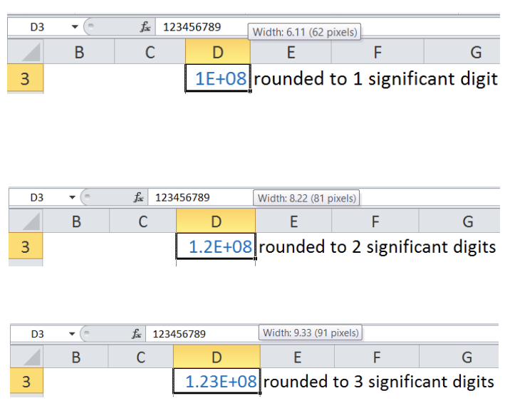 Figure 8. A large number displayed with different number of significant digits based on column width
Work-around:
To stop Excel from rounding a whole number, we can adjust the column width to display all the digits.
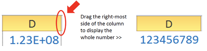 Figure 9. Adjusting column width to display the entire number
Stop Excel From Rounding Currency
Most currencies have two decimal places. Rounding currencies might have a small impact since it will only be dealing with tenths or hundredths of a currency, such as centavos.
There are instances, however, where rounding currencies becomes serious. In Accounting, for example, in order to arrive at a more accurate result, rounding should be done only as needed, or as late into the calculations as possible.
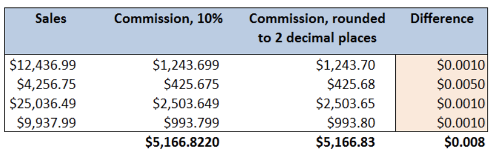 Figure 10. Sample calculation showing the difference with rounded numbers
The table above shows the effect of rounding currencies into the total commission.
Work-around:
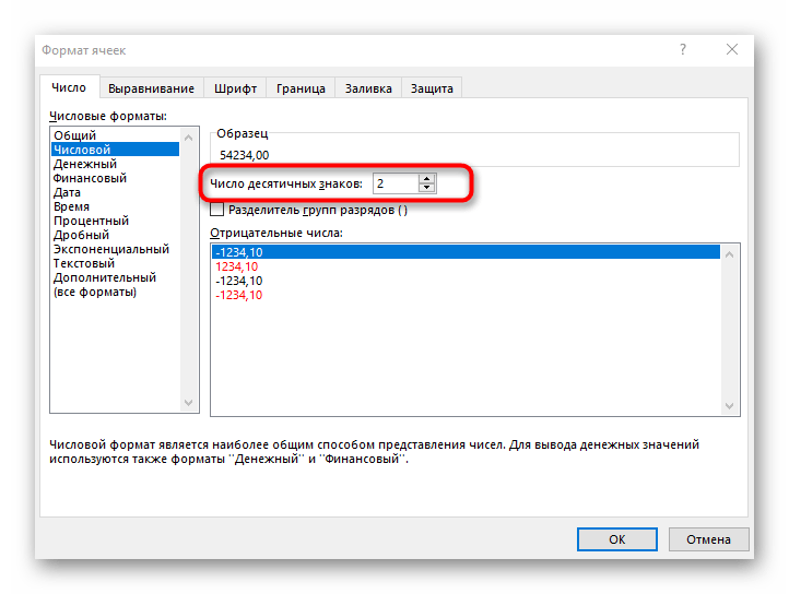
To stop Excel from rounding currencies, format the decimal places to “3 or more”. This way, the precision and accuracy of our data is preserved as close to the original value as possible.
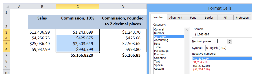 Figure 11. Setting the decimal places to display the whole value of currencies
Most of the time, the problem you will need to solve will be more complex than a simple application of a formula or function. If you want to save hours of research and frustration, try our live Excelchat service! Our Excel Experts are available 24/7 to answer any Excel question you may have. We guarantee a connection within 30 seconds and a customized solution within 20 minutes.
Содержание
- Способ 1: Функция «Увеличить разрядность»
- Способ 2: Настройка формата ячеек
- Способ 3: Изменение формата ячеек
- Вопросы и ответы

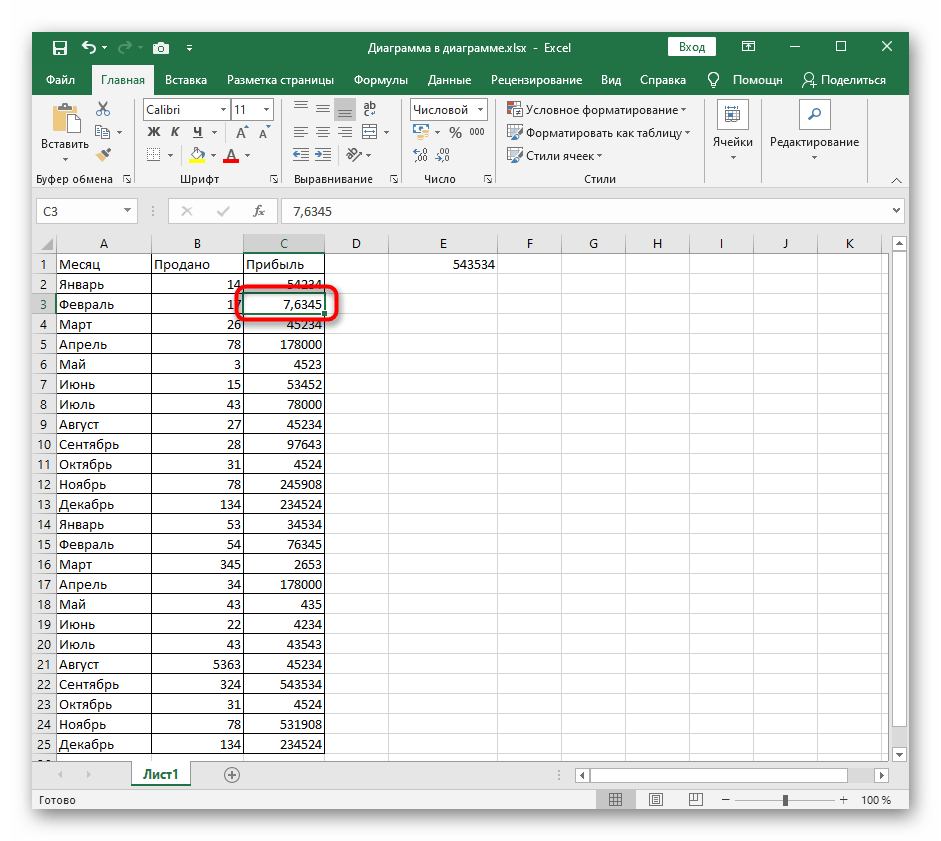
Способ 1: Функция «Увеличить разрядность»
Самый простой и быстрый способ отключения округления чисел в Excel — использование функции «Увеличить разрядность». Она работает по принципу увеличения отображения чисел после запятой до необходимого количества, а для использования понадобится выполнить пару действий.
- Определитесь, для каких ячеек требуется вносить изменения, и если их несколько, выделите все сразу.
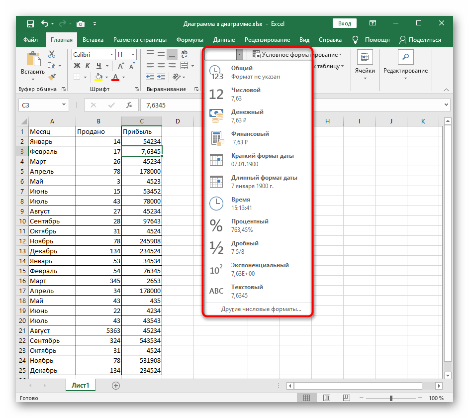
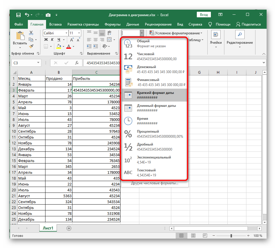
- В блоке «Число» разверните список числовых форматов и решите, какой хотите использовать.
- Сразу же после этого нажмите по кнопке «Увеличить разрядность» столько раз, сколько чисел хотите добавить.
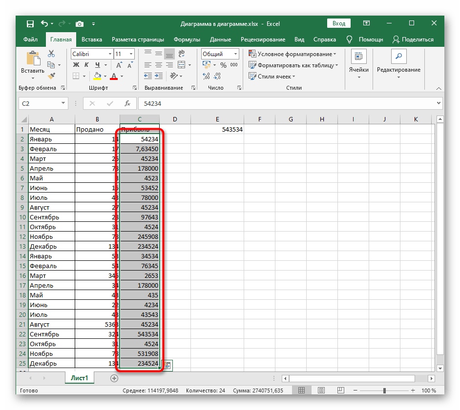
- Отслеживайте изменения, просматривая состояние ячеек, и учитывайте, что как только округление отключится полностью, каждый следующий добавляемый знак будет «0».


Точно по так же функционирует и другая опция, предназначенная для уменьшения разрядности. Она расположена на этой же панели и ей можно воспользоваться, если вдруг вы добавили несколько лишних знаков.
Способ 2: Настройка формата ячеек
Настройка формата ячеек позволяет установить точное количество знаков после запятой, чтобы задать автоматическое округление. Ничего не помешает увеличить их количество до требуемого, отключив тем самым округление. Для этого понадобится обратиться к соответствующему меню в Excel.
- В первую очередь всегда выделяйте те ячейки, для которых будут применены последующие изменения.
- Далее разверните меню «Ячейки» и выберите выпадающее меню «Формат».
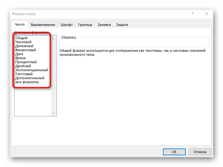
- В нем кликните по последнему пункту «Формат ячеек».
- Выделите левой кнопкой мыши тот числовой формат, который используется для выделенных ранее ячеек.
- Установите количество десятичных знаков, вписав его значение в отведенном для этого поле, примените новые настройки и покиньте текущее меню.
- Взгляните на выделенные ранее ячейки и убедитесь в том, что теперь их значения отображаются корректно.


Способ 3: Изменение формата ячеек
Завершает статью вариант, подразумевающий изменение формата ячеек с числами, для которых отключается округление. Это единственный доступный метод, который окажется эффективным, если округление происходит по причине недостаточного места в ячейке для всех знаков.
Вы можете воспользоваться предыдущим способом, выбрав другой формат ячеек, но при этом с результатом можно будет ознакомиться только после выхода из меню. В качестве альтернативы советуем развернуть меню «Число», о котором уже говорилось в Способе 1, и посмотреть представление чисел для других форматов. Нажмите по тому, который окажется подходящим, чтобы он сразу вступил в действие.

Учитывайте, что если числу задать текстовый формат, не получится рассчитать его сумму при выделении или использовать ячейку в математических формулах. Если же в будущем потребуется снова округлить числа, воспользуйтесь другой инструкцией на нашем сайте, перейдя по ссылке ниже.
Подробнее: Округление чисел в Microsoft Excel
Еще статьи по данной теме:
Помогла ли Вам статья?
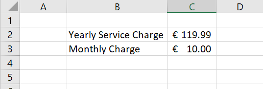
Hello, welcome to another #formulafriday blog post for some more formula fun on a Friday – why not?. Today let’s take a look and explore the issue of Excel rounding or not rounding numbers. You may have come across this in Excel especially when working with currency values. Rounding your values may work in some scenarios, but you may NOT want to round up figures in some circumstances. Take a look at an example, you may have a yearly charge of a service, which is split between 12 monthly payments. See my screenshot below.
Excel Rounding- Do You Want It?
The example above Excel has rounded the monthly charge to 10. This is not pricing that the sales department want to promote the service at in their online advertisement. Excel will automatically round the numbers if the column is not wide enough to display the entire number, or when it’s format is set to show a smaller number of decimal places than the original number contains.
If you enter a number into a worksheet cell that has General formatting, like all cells in a new worksheet, the number will be rounded so it fits into the cell. In the case of our promotion of monthly service the display in the cell is 10 but in the formula bar, you can see that the actual entire number is still available in full.
To toggle between seeing the formula and the result of the formula in the formula bar you can click into the formula bar then hit the F9 button. Hit the ESC key to return to the display to the formula again.
Using The TRUNC Function.
The TRUNC function returns a truncated number based on a given number of digits. The Syntax of TRUNC is
=TRUNC (number, [num_digits]) where
number = the number to truncate
num_digits = an optional argument with which to determine the precision of the truncation. The default is 0.
TRUNC removes the fractional part of the number and returns just the integer. For example,
4.9 would return 4
5.25 would return 5
As you can see this is a lot different to the automatically rounded numbers that Excel usually displays. So, if you want only the integer part of your number use TRUNC. Back to our online sales example. The sales department do want to use the monthly payments of 10.00 that Excel rounds to automatically instead we have to force the 9.99 offer they want to market to their online customers. Ok, so that is no problem for us now. As well as just returning integers TRUNC can also be used with the optional argument num_digits. This will return a specified number of decimal places, again with no rounding.
The Solution!
So we can use the TRUNC formula for our problem as we can specify that it uses 2 as the optional argument as the number of digits.
Our formula would look like this
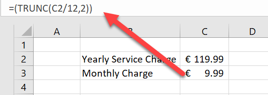
Solved!. We can keep the sales department happy.
If you want more Excel and VBA tips then sign up for my Monthly Newsletter where I share 3 Tips on the first Wednesday of the month and receive my free Ebook, 30 Excel Tips.

If you want to see all of the blog posts in the Formula Friday series. Click on the link below
How To Excel At Excel – Formula Friday Blog Posts.


Do You Need Help With An Excel Problem?.
I am pleased to announce I have teamed up with Excel Rescue, where you can get help with Excel FAST.

Microsoft has designed excel in a way that will be efficient and easy to use for its users. However, some of the features of Excel can be counterproductive and thus reducing its efficiency. Rounding off large numbers is one of these features that are times counterproductive. When dealing with large numbers on excel cells, excel decides to round off the number hence not displaying the exact number inputted. This may be brought about by issues like; the number inputted is too large to be accommodated by the cell’s width and the cell formatted nature of rounding off large numbers.
To stop excel from rounding off numbers is possible and can be achieved by altering the cell’s settings. Let us now discuss the procedure to be followed in doing this.
1. Open the excel
Double click the Excel app icon, which resembles a green with a white «X» on it. And then, open either a new document or an existing document on your device that you want to change the cell setting.
2. Input your large numbers
On the blank screen of excel, choose and select any blank cell to input the number. Within the cell, input the number of any length and click anywhere outside the cell to save the cell’s data. As expected, Excel will automatically convert the large number into a smaller rounded-off number. Now it’s upon the user to alter the settings to regain the original large number.

3. Click the cell
Click the cell that contains the rounded-off number. Then, right-click to access the cell’s side setting.
4. Click the Format cells button
On the side setting, locate and click on the format cells button. This is where the entire cell’s setting and other cell features are contained.

5. Tap the number tab
On the format cells screen, locate and tap the number bar on the top leftmost most of the screen. And then, select the number button on the left side of the page.

6. Change the decimal places figures
If you’re working with data that contains decimal places, click the up or down button next to «Decimal places» and then adjust/increase the decimal place figures according to your data. Then, click «OK» to save changes. Otherwise, if you’re working with large whole numbers, you can alter the cell settings by only clicking the «OK» button without altering with any other setting on this screen.
Your data on the selected cell will be converted to its original format by clicking the OK button.

Also, once you’ve changed the data on that cell, all the cells found in the same column will be formatted. Thus, you can enter large numbers on that column without having to change the cell setting. This makes it easier and more efficient for the user to input large numbers on the same column.
