Excel for Microsoft 365 Excel 2021 Excel 2019 Excel 2016 Excel 2013 Excel 2010 Excel 2007 More…Less
Operators specify the type of calculation that you want to perform on the elements of a formula. Excel follows general mathematical rules for calculations, which is Parentheses, Exponents, Multiplication and Division, and Addition and Subtraction, or the acronym PEMDAS (Please Excuse My Dear Aunt Sally). Using parentheses allows you to change that calculation order.
Types of operators. There are four different types of calculation operators: arithmetic, comparison, text concatenation, and reference.
-
Arithmetic operators
To perform basic mathematical operations, such as addition, subtraction, multiplication, or division; combine numbers; and produce numeric results, use the following arithmetic operators.
Arithmetic operator
Meaning
Example
+ (plus sign)
Addition
=3+3
– (minus sign)
Subtraction
Negation=3–3
=-3* (asterisk)
Multiplication
=3*3
/ (forward slash)
Division
=3/3
% (percent sign)
Percent
30%
^ (caret)
Exponentiation
=3^3
-
Comparison operators
You can compare two values with the following operators. When two values are compared by using these operators, the result is a logical value—either TRUE or FALSE.
Comparison operator
Meaning
Example
= (equal sign)
Equal to
=A1=B1
> (greater than sign)
Greater than
=A1>B1
< (less than sign)
Less than
=A1<B1
>= (greater than or equal to sign)
Greater than or equal to
=A1>=B1
<= (less than or equal to sign)
Less than or equal to
=A1<=B1
<> (not equal to sign)
Not equal to
=A1<>B1
-
Text concatenation operator
Use the ampersand (&) to concatenate (join) one or more text strings to produce a single piece of text.
Text operator
Meaning
Example
& (ampersand)
Connects, or concatenates, two values to produce one continuous text value
=»North»&»wind» results in «Northwind».
Where A1 holds «Last name» and B1 holds «First name», =A1&», «&B1 results in «Last name, First name». -
Reference operators
Combine ranges of cells for calculations with the following operators.
Reference operator
Meaning
Example
: (colon)
Range operator, which produces one reference to all the cells between two references, including the two references.
B5:B15
, (comma)
Union operator, which combines multiple references into one reference
=SUM(B5:B15,D5:D15)
(space)
Intersection operator, which produces one reference to cells common to the two references
B7:D7 C6:C8
Need more help?
‘Less Than or Equal to’ operator (<=) is one of the six logical operators (also known as the comparison operators) used in Microsoft Excel to compare values. The “<=” operator checks if the first value is less than or equal to the second value and returns ‘TRUE’ if the answer is yes or else ‘FALSE’. This is a boolean expression, so it can only return either TRUE or FALSE.
The ‘less than or equal to’ is used to perform the various logical operations in Excel. It is rarely used alone, and it is often combined with other Excel functions such as IF, OR, NOT, SUMIF, and COUNTIF, etc. to perform powerful calculations. In this tutorial, we will see how to use the ‘less than or equal to (<=)’ operator with text, date, and number as well as with Excel functions.
Compare Text Values with ‘<=’ Operator in Excel
The ‘less than or equal to’ operator can be used to compare text values in Excel. Before you compare values text values in Excel, you should know that all logical operators are case-insensitive. It means they ignore case differences when comparing text values.
There’s another thing, you should know when comparing text strings with logical operators in Excel. MS Excel considers the first alphabet “a” as the smallest value and the last alphabet “z” as the largest value. That means a < d, r < v, k > j, etc. Let us explain with an example.
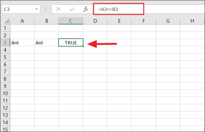
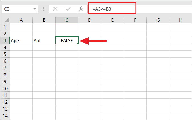
Example 1: If you want to check the text value in cell A3 is less than or equal to the value in cell B4, use this simple formula:
=A3<=B3An excel formula must always start with an equal sign ‘=’. The first argument is cell A3, the second argument is cell B3, and the operator is placed in between. Since both values are the same, the result is ‘TRUE’.
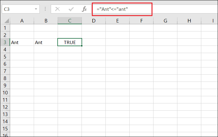
Instead of using cell references, you can also use direct text value as arguments in the formula. But when a text value is inserted in a formula, it must always be enclosed in double quotation marks like this:
="Ant"<="ant"Since logical operators are case-insensitive, it ignores the case differences and returns TRUE as the result.
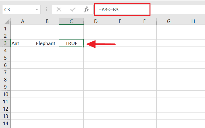
Example 2:
In the below example, “Ant” text is definitely not equal to “Elephant”. So you may be wondering, but how Ant is less than Elephant? Is it because it’s small? No, the first letter of cell A3 (“A”) is smaller than the first letter of cell B3 (“E”).
As we mentioned before, Excel considers that letters later in the alphabet are larger than earlier letters. Here, the formula compares the first letter of the A3 with the first letter of B3. The first letter ‘A’ < first letter ‘E’, so the formula returns ‘TRUE’.
Example 3:
When comparing texts, Excel starts with the first letter of the texts. If they are identical, it goes to the second letter. In this example, the first letter of A3 and B3 are the same, so the formula moves to the second letter of A3 and B3. Now, “p” is not less than “n”, hence, it returns ‘FALSE’.
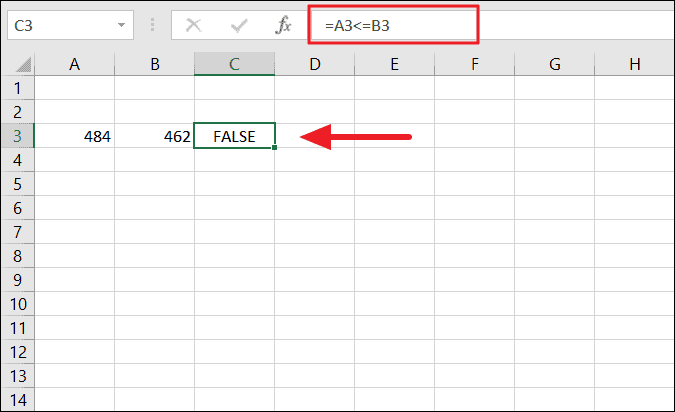
Compare Numbers with ‘<=’ Operator in Excel
Using ‘less than or equal to’ with numbers is simple enough anyone can do it. You can also use this operator to build complex mathematical operations in Excel.
Here’s an example to compare to numbers with ‘<=’:
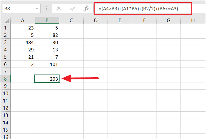
You can use the ‘less than or equal’ operator with mathematical operators as well as other logical operators to create complex mathematical operations.
For example, try this formula:
=(A4>B3)+(A1*B5)+(B2/2)+(B6<=A3)In mathematical calculations, the result of logical operation ‘TRUE’ is the equivalent of 1, and FALSE is 0.
That means, first part of the formula (A4>B3) returns ‘0’ and the last part of the formula (B6<=A3) returns ‘1’. And our formula would look like this:
=0+(A1*B5)+(B2/2)+1And the returning result would be ‘203’.
Compare Dates with ‘<=’ Operator in Excel
Besides text and numbers, you can also use the ‘less than or equal to’ operator to compare date values. Logical operators can also be used to compare between data types, like date and text or number and text, etc.
One thing you should know when comparing dates is that Excel saves dates and time as numbers, but they are formatted to look like dates. Excel date number starts from 1st of January 1900 12:00 AM, which is saved as 1, 2nd of January 1900 is saved as 2, and so on.
For instance, here a list of dates entered in Excel.
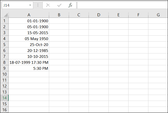
To see the numbers behind dates, press the shortcut keys Ctrl + ~ on the keyboard or change the format of the date to number or general. And you will see numbers of the above dates entered in excel as shown below.
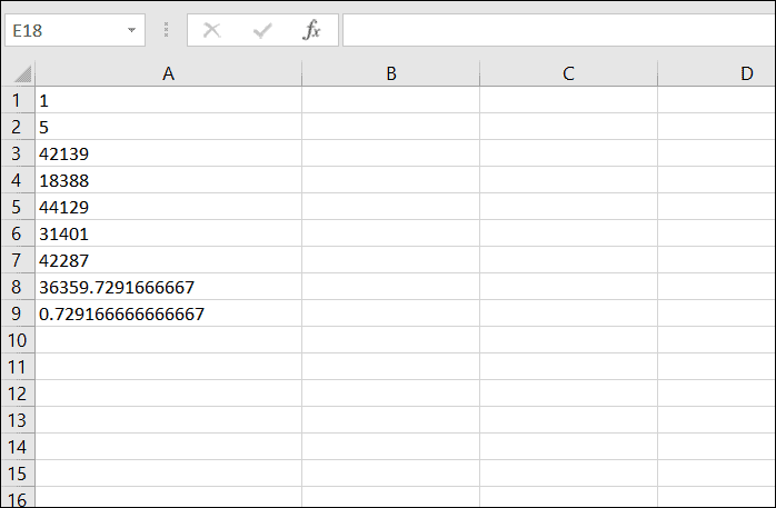
Excel uses these numbers whenever a date is involved in a calculation.
Let’s take a look at this table:
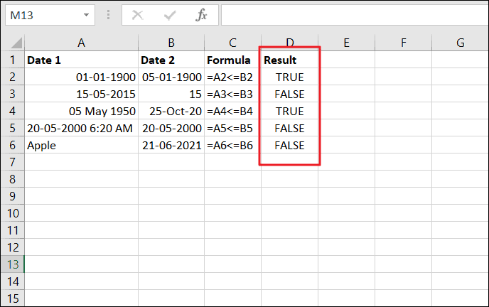
- C2: A2 date is less than the B2, hence, TRUE.
- C3: A3 (which number is 42139) is greater than B3 – FALSE.
- C4: A4 is less than B4 – TRUE.
- C5: A5 (36666.263) is greater than B5 (36666). When only a date is entered, its default time is 12:00 AM, which is midnight. So the answer is FALSE
- C6: A6 is greater than B6. Because a text is always considered as the largest value when compared to any number or date in Excel. Hence, it’s FALSE.
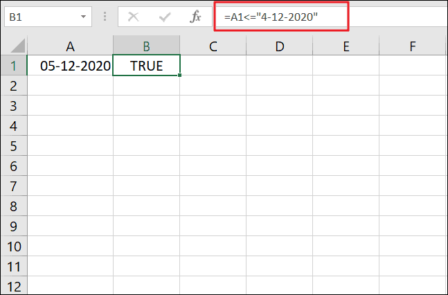
Sometimes, when you comparing a date value with a cell, Excel may consider the date value as a text string or arithmetic calculation.
In the below example, even though A1 is greater than “4-12-2020”, the result is “TRUE”. Because Excel considers the value as a text string.
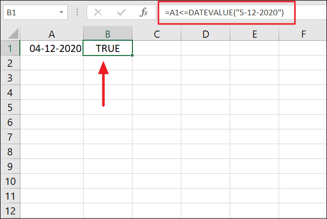
Also, here the date part (5-12-2020) in the formula is considered as a mathematical calculation:

To fix this, you need to enclose a date in the DATEVALUE function, like this:
=A1<=DATEVALUE("5-12-2020")Now, you would get the correct result:
Using ‘Less Than or Equal To’ Operator with Functions
In excel, logical operators (like <=) are widely used in parameters of Excel functions such as IF, SUMIF, COUNTIF, and many other functions to perform powerful calculations.
Using ‘<=’ with IF Function in Excel
The ‘<=’ operator can be used within the ‘logic_test’ argument of the IF function to perform logical operations.
The Excel IF function evaluates a logical condition (which is made by ‘less than or equal to’ operator) and returns one value if the condition is TRUE, or another value if the condition is FALSE.
The syntax for the IF function is:
=IF(logical_test,[value_if_true],[value_if_false])Let’s assume, you have a list of student mark lists, and you want to check whether each student is passed or failed based on their test score. To do that, try this formula:
=IF(B2<=50,"Fail","Pass")The passing mark is ’50’ which is used in the logical_test argument. The formula checks, if the value in B2 is less than or equal to ’50’, and returns ‘Fail’ if the condition is TRUE or returns ‘Pass’ if the condition is FALSE.
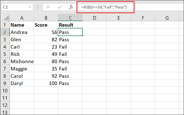
And the same formula is applied to the rest of cells.
Here’s another example:
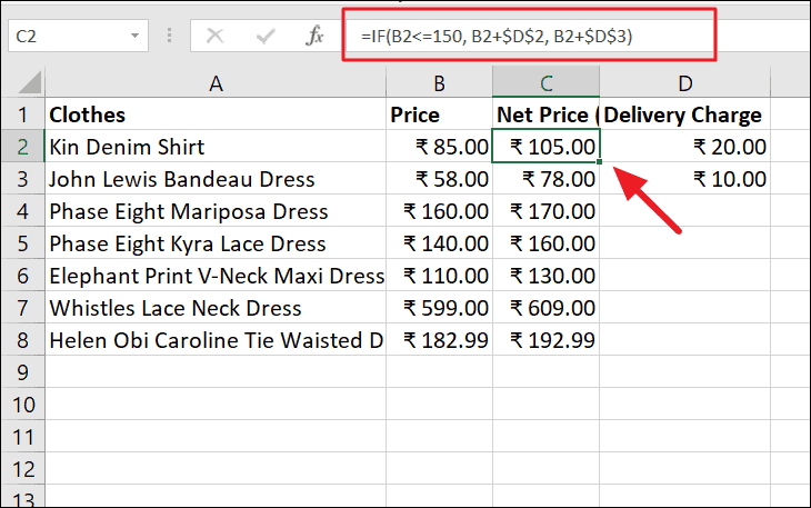
For example, let’s say we have a clothes order list with prices. If the price of a dress is less than or equal to $150, we need to add a $20 delivery charge to the net price or add a $10 delivery charge to the price. Try this formula for that:
=IF(B2<=150, B2+$D$2, B2+$D$3)Here, if the value in B2 is less than or equal to 150, the value in D2 is added to B2, and the result is displayed in C2. If the condition is FALSE, then D3 is added to B2. We added the ‘$’ sign before the column letters and row numbers of cell D2 and D3 ($D$2, $D$3) to make them absolute cells, so it doesn’t change when copying the formula to the rest of the cells (C3:C8).
Using ‘<=’ with SUMIF Function in Excel
Another Excel function that logical operators are more commonly used with is the SUMIF function. The SUMIF function is used to sum a range of cells when corresponding cells match a certain condition.
The general structure of SUMIF function is:
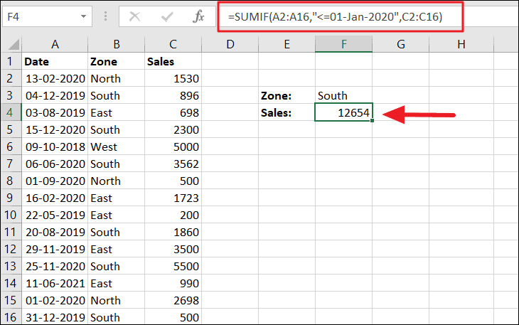
=SUMIF(range,criteria,[sum_range])For example, let’s say you want to sum all the sales that happened on or before (<=) January 01, 2019, in the below table, you can use the ‘<=’ operator with SUMIF function to sum all values:
=SUMIF(A2:A16,"<=01-Jan-2020",C2:C16)The formula check looks for all sales that occurred on or before (<=) 01-Jan-2020 in the cell range A2:A16 and sums all the sales amounts corresponding to those matching dates in the range C2:C16.
Using ‘<=’ with COUNTIF Function in Excel
Now, let’s use the logical operator ‘less than or equal to’ with the COUONTIF function. Excel COUNTIF function is used to counts the cells that meet a certain condition in a range. You can use the ‘<=’ operator to count the number of cells with a value that is less than or equal to the specified value.
The Syntax of COUNTIF:
=COUNTIF(range,criteria)You have to write a condition using the ‘<=’ operator in the criteria argument of the function and the range of cells where you count the cells in the range argument.
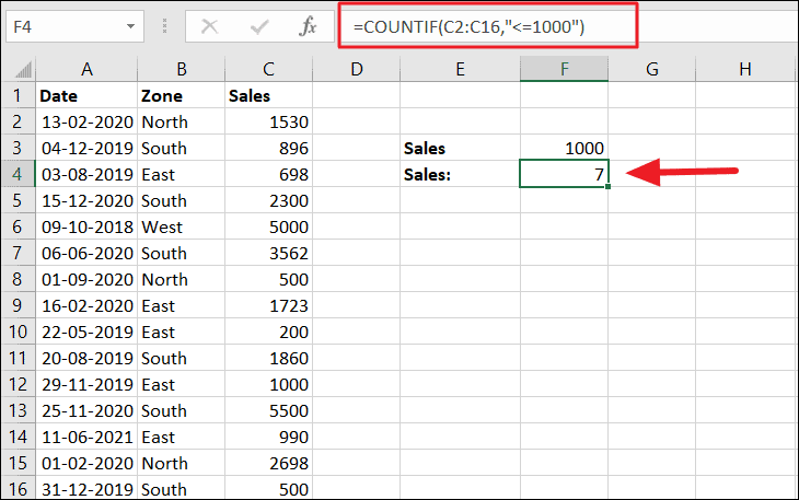
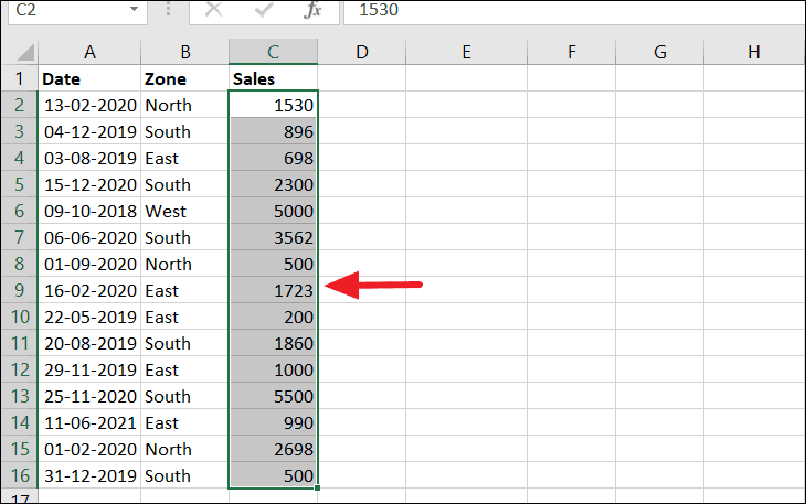
Suppose you want to count the sales that are less than or equal to 1000 in the below example, then you can use this formula:
=COUNTIF(C2:C16,"<=1000")The above formula counts cells that are less than or equal to 1000 in the range C2 to C16 and displays the result in cell F4.
You can also count cells by comparing a criterion value in a cell against a range of cells. In such cases, write criteria by joining the operator (<=) and a reference to the cell containing the value. To do that, you need to enclose the comparison operator in double quotes (“”), and then place an ampersand (&) sign between the logical operator (<=) and the cell reference.
=COUNTIF(C2:C16,"<="&F3)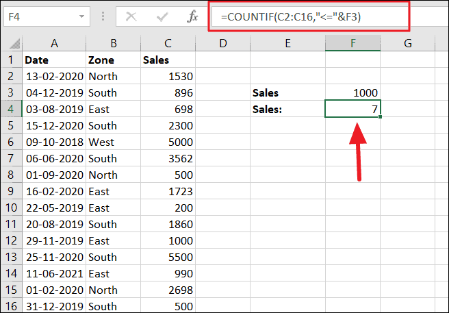
Besides IF, SUMIF, and COUNTIF functions, you also use the ‘less than or equal’ operator with other less used functions such as AND, OR, NOR, or XOR, etc.
Using ‘<=’ Operator in Excel Conditional Formatting
Another common use for the ‘less than or equal to’ operator is in Excel Conditional Formatting which helps you highlight or differentiate data stored in your worksheet based on a condition.
For example, if you want to highlight the sales amounts that are less than or equal to ‘2000’ in column C, you have to write a simple rule using the ‘<=’ operator in Excel Conditional Formatting. Here’s how you do that:
First, select the cell range of cells where you want to apply a rule (condition) and highlight data (In our case C2:C16).
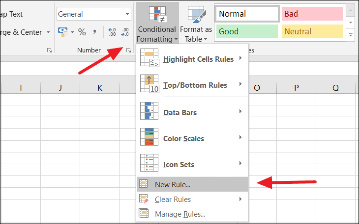
Then go to the ‘Home’ tab, click ‘Conditional Formatting’ and select ‘New Rule’ from the drop-down.
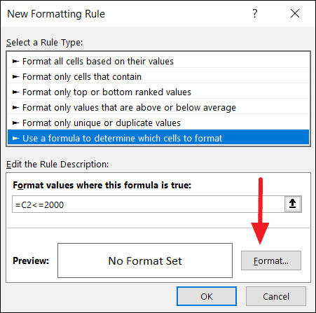
In the New Formatting Rule dialog box, select the ‘Use a formula to determine which cells to format’ option under the Select a Rule Type section. Then, type the below formula to highlight sales that are less than or equal to 2000 in the ‘Format values where this formula is true’ box:
=C2<=2000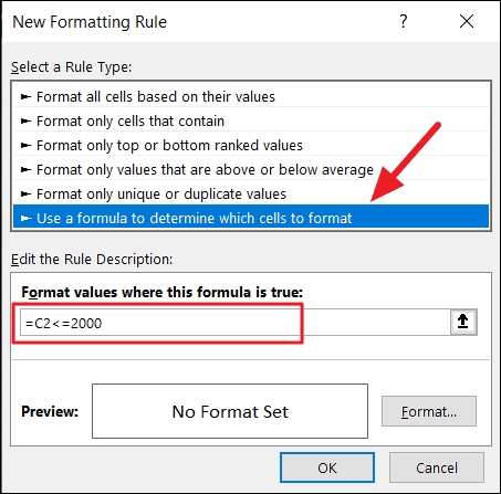
After you enter the rule, click the ‘Format’ button to specify the formatting.
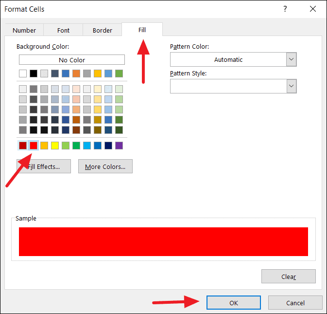
In the Format Cells dialog box, you can choose the specific formatting you want to apply to highlight cells. You can change the number format, font format, borders style, and fill the color of the cells. Once, you have chosen the format, click ‘OK’.
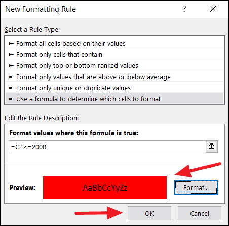
Back in the New Formatting Rule dialog, you can see the preview of your selected format. Now, click ‘OK’ again to apply the formatting and highlight the cells.
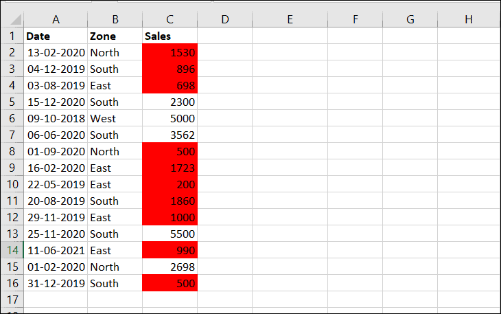
As you can see, the sales that are less than or equal to 2000 are highlighted in column C.
As you have learned, the ‘<=’ operator is quite easy and useful in Excel to perform calculations.
That’s it.
Logical operators in Excel are also known as comparison operators. They are used to compare two or more values. The return output given by these operators is either TRUE or FALSE. We get a TRUE value when the conditions match the criteria and FALSE as a result when the conditions do not match the criteria.
Below are the most commonly used logical operators in Excel.
Now we will look at each one of them in detail.
| Sr No. | Logical Operator Excel Symbol | Operator Name | Description |
|---|---|---|---|
| 1 | = | Equal to | Compares One Value to Other Value |
| 2 | > | Greater Than | Tests whether the value is greater than a certain value or not |
| 3 | < | Less Than | Tests whether the value is less than a certain value or not |
| 4 | >= | Greater Than or Equal To | Tests whether the value is greater than or equal to a certain value or not |
| 5 | <= | Less Than or Equal To | Tests whether the value is less than or equal to a certain value or not |
| 6 | <> | Not Equal To | Tests whether a particular value is not equal to a certain value or not |
Table of contents
- List of Logical Excel Operators
- #1 Equal Sign (=) to Compare Two Values
- #2 Greater Than (>) Sign to Compare Numerical Values
- #3 Greater Than or Equal To (>=) Sign to Compare Numerical Values
- #4 Less than Sign (<) to Compare Numerical Values
- #5 Less Than or Equal To Sign (<=) to Compare Numerical Values
- #6 Not Equal Sign (<>) to Compare Numerical Values
- Logical Operator in Excel with Formulas
- #1 – IF with Equal Sign
- #2 – IF with Greater Than Sign
- #3 – IF with Less Than Sign
- Things to Remember
- Recommended Articles
You can download this Excel Operators Template here – Excel Operators Template
#1 Equal Sign (=) to Compare Two Values
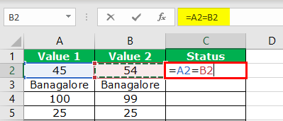
We can use the equal sign (=) to compare one cell value against the other cell value. In addition, we can compare all types of values using an equal sign. For example, assume we have the below values from cells A1 to B5.
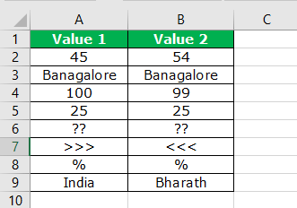
Now, we want to test whether the value in cell A1 is equal to cell B1’s value.
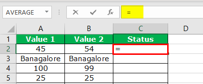
- To select the value of A1 to B1, let us open the formula with an equal sign.

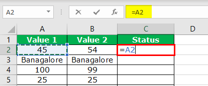
- Now, select cell A1.

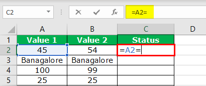
- Now, type the one more logical operator symbol equal sign (=).

- Now, select the second cell we are comparing, the B2 cell.

- Press the “Enter” key to close the formula. Then, we must copy and paste it into other cells.

So, we get “TRUE” as a result if the cell 1 value is equal to cell 2 or we get “FALSE.”
#2 Greater Than (>) Sign to Compare Numerical Values
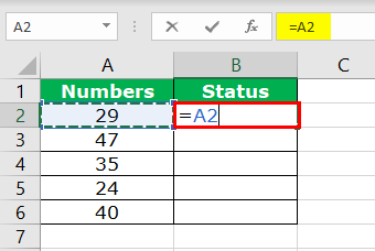
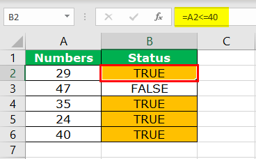
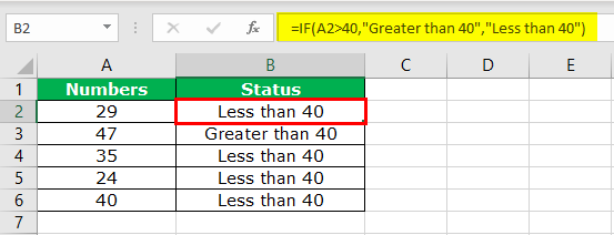
Unlike equal sign (=) greater than sign (>) can only test numerical values, not text values. So, for example, if the values are in cells A1 to A5 and we want to try whether these values are greater than (>) the value of 40 or not.

- Step 1: We must first open the formula in the B2 cell and select cell A2 as the cell reference.
- Step 2: Since we are testing, the value is greater than the mention > symbol and apply the condition as 40.
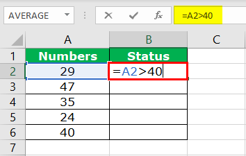
- Step 3: Now, close the formula and use it to remain cells.
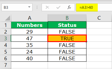
Only one value is >40, i.e., cell A3 value.
Cell A6 value is 40; since we have applied the logical operator > as the criteria formula returned, the result is FALSE. We will see how to solve this issue in the next example.
#3 Greater Than or Equal To (>=) Sign to Compare Numerical Values
In the previous example, the formula returns a TRUE value only to those greater than the criteria value. But if the criteria value is also included in the formula, we need to use the >= symbol.
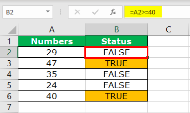
The previous formula excluded the value of 40, but this formula included.
#4 Less than Sign (<) to Compare Numerical Values
Like how greater than tests the numerical values are, similarly less than also tests the numbers. We have applied the formula as <40.
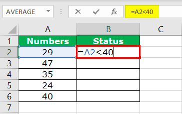
It works opposite to the greater than criteria. It has returned TRUE to all those values that are less than 40.

#5 Less Than or Equal To Sign (<=) to Compare Numerical Values
Like how >= sign includes the criteria value in the formula similarly, <= also performs the same way.
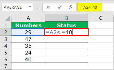
This formula had the criteria value, so the value of 40 is returned as TRUE.
#6 Not Equal Sign (<>) to Compare Numerical Values
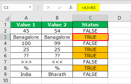
Combination of greater than (>) and less than (<) signs make the operator sign not equal to <>. It works opposite to an equal sign. The equal sign (=) tests whether the one value is equal to the other value and returns TRUE, whereas not equal to sign <> returns TRUE if the one value is not equal to another value and returns FALSE if the one value is not equal to another one.
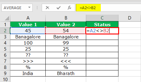
As we said, A3 and B3 cell values are the same, but the formula returns FALSE, which is completely different from the EQUAL sign logical operator.

Logical Operator in Excel with Formulas
We can also use logical operator symbols in other Excel formulas IF Excel function is one of the often used formulae with logical operators.
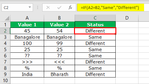
#1 – IF with Equal Sign
Suppose the function tests whether the condition is equal to a certain value or not. If the value is equal, then we can have our value. Below is a simple example of that.
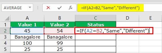
The formula returns the Same if the cell A2 value is equal to the B2 value; if not, it will return Different.
#2 – IF with Greater Than Sign
We can test certain numerical values, arrive at results if the condition is TRUE, and return a different result if the condition is FALSE.
#3 – IF with Less Than Sign
The below formula will show the logic of applying if with less than the logical operators.

Things to Remember
- Excel logical operator symbols return only TRUE or FALSE.
- Combination of > & < symbols do not equal sign <>.
- >= & <= sign includes the criteria also in the formula.
Recommended Articles
This article is a guide to Logical Operators in Excel. We discuss the top 6 types of MS Excel logical operators, practical examples, and a downloadable Excel template. You may learn more about Excel from the following articles: –
- How Not Equal to Works in Excel VBA?
- Greater Than or Equal to in Excel
- Divide Formula in Excel
- Multiply in Excel Formula
- Quotient in Excel
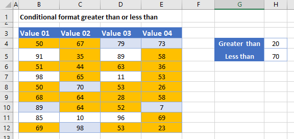
This tutorial will demonstrate how to highlight cells based on whether they are greater than or less than another cell using Conditional Formatting in Excel and Google Sheets.
Use a Highlight Cell Rule
To highlight cells where the value is greater than a specified number, you can use one of the built in Highlight Cell rules within the Conditional Formatting menu.
Greater Than
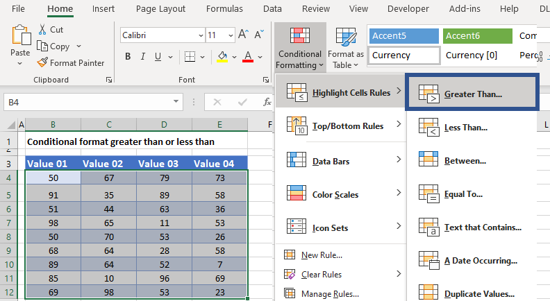
- Select the range to apply the formatting (e.g., B4:E12).
- In the Ribbon, select Home > Conditional Formatting > Highlight Cells Rules > Greater Than…
- You can either type in the value, or to make the formatting dynamic (i.e., the result will change if you change the values), you can click on the cell that contains the value you require.
- Select the type of formatting you require from the drop down box and click OK.
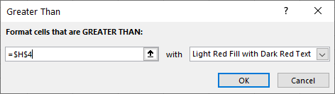
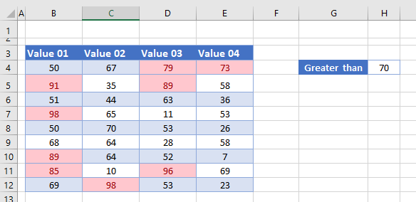
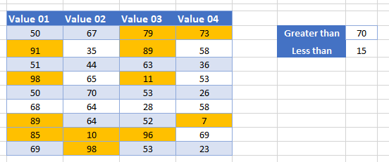
The table now indicates which values are greater than that in cell H4 (20) by making them red.
- Change the value in H4 to obtain a different result.
Less Than
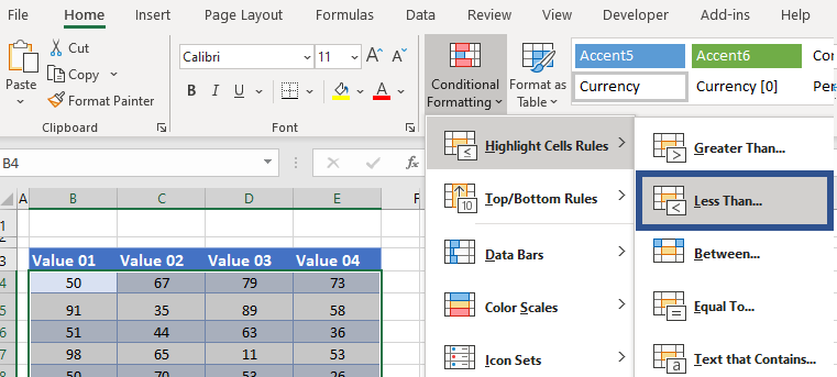
- Select the range to apply the formatting.
- In the Ribbon, select Home > Conditional Formatting > Highlight Cells Rules > Less Than…
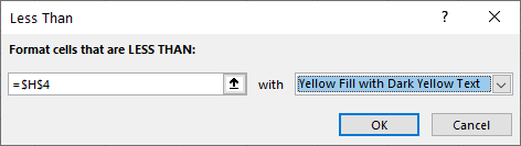
- As before, click on the cell that contains the value you require.
- Click OK to format the cells with the desired formatting.
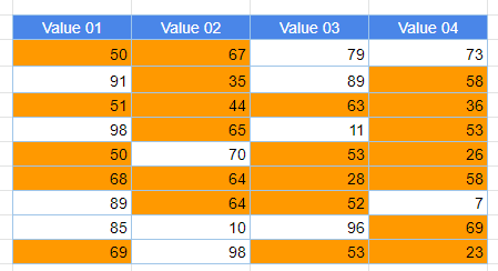
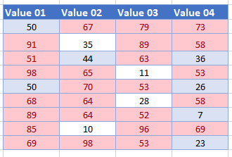
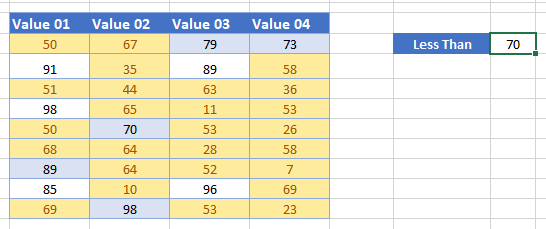
The resulting formatting shows numbers less than 70 in yellow.
Highlight Cells With a Custom Function
With Conditional Formatting, you can also highlight cells by using a custom function.
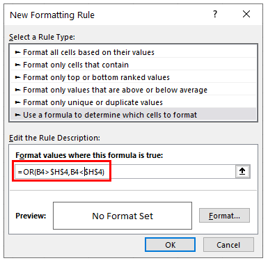
Greater Than AND Less Than
You can highlight cells that have a greater value than one cell, but a smaller value than another by creating a New Rule and selecting Use a formula to determine which cells to format.
- Select the range to apply the formatting.
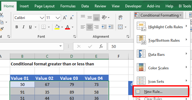
- In the Ribbon, select Home > Conditional Formatting > New Rule.
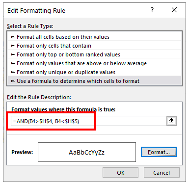
- Select Use a formula to determine which cells to format, and enter this formula that uses the AND Function:
=AND(B4>$H$4, B4<$H$5)- You need to lock the reference to cells H4 and H5 by making them absolutes. Do this by using the $ sign around the row and column indicators, or by pressing F4 on the keyboard.
- Finally, click on the Format button.
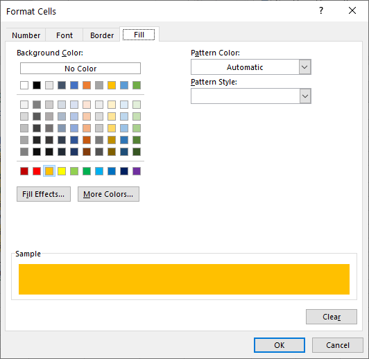
- Select the formatting you want for numbers between H4 (20) and H5 (70). Click OK.
The result is similar to the previous examples, just highlighting on a different condition.
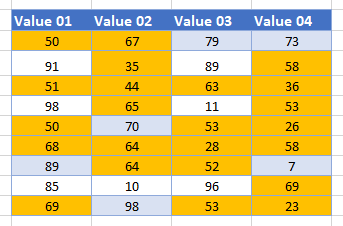
Greater Than OR Less Than
To highlight cells that have a greater value than one cell or have a smaller value than another cell (i.e., outside the range of the two cells), follow these steps:
- Select the range to apply the formatting.
- In the Ribbon, select Home > Conditional Formatting > New Rule
- Select Use a formula to determine which cells to format, and enter this formula that uses the OR Function:
=OR(B4>$H$4, B4<$H$5)- Once again, lock the reference to cells H4 and H5 by making them absolutes. Use the $ sign around the row and column indicators, or press F4 on the keyboard.
- Click on the Format button.
- Select the formatting you want for numbers that are not between H4 (20) and H5 (70). Click OK.
Highlight Cells With a Custom Function in Google Sheets
The process to highlight cells with a greater value than one cell, and a smaller value than another cell in Google Sheets is similar to the process in Excel.
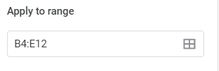
- Highlight the cells you wish to format, and then click on Format > Conditional Formatting.
- The Apply to Range section will already be filled in.
- From the Format Rules section, select Custom Formula from the drop-down list and type in the following formula:
=AND(B4>$H$4, B4<$H$5)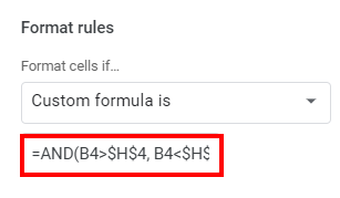
Once again, use the absolute signs (dollar signs) to lock in the values in H4 and H5.
- Select the fill style for the cells that meet the criteria.
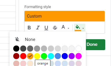
- Click Done to apply the rule.