Not in list function in excel - Word и Excel - помощь в работе с программами

So, there are times when you would like to know that a value is in a list or not. We have done this using VLOOKUP. But we can do the same thing using COUNTIF function too. So in this article, we will learn how to check if a values is in a list or not using various ways.

Check If Value In Range Using COUNTIF Function

So as we know, using COUNTIF function in excel we can know how many times a specific value occurs in a range. So if we count for a specific value in a range and its greater than zero, it would mean that it is in the range. Isn’t it?

Generic Formula

=COUNTIF(range,value)>0

Range: The range in which you want to check if the value exist in range or not.

Value: The value that you want to check in the range.

Let’s see an example:

Excel Find Value is in Range Example

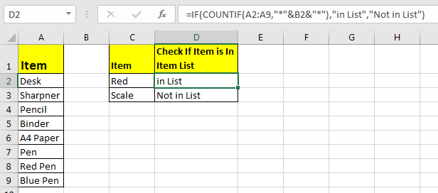
For this example, we have below sample data. We need a check-in the cell D2, if the given item in C2 exists in range A2:A9 or say item list. If it’s there then, print TRUE else FALSE.

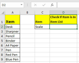
Write this formula in cell D2:

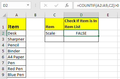
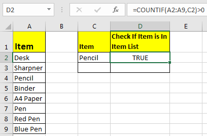
Since C2 contains “scale” and it’s not in the item list, it shows FALSE. Exactly as we wanted. Now if you replace “scale” with “Pencil” in the formula above, it’ll show TRUE.

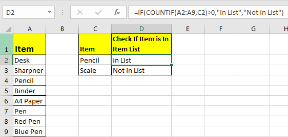
Now, this TRUE and FALSE looks very back and white. How about customizing the output. I mean, how about we show, “found” or “not found” when value is in list and when it is not respectively.
Since this test gives us TRUE and FALSE, we can use it with IF function of excel.

Write this formula:

=IF(COUNTIF(A2:A9,C2)>0,»in List»,»Not in List»)

You will have this as your output.

What If you remove “>0” from this if formula?

=IF(COUNTIF(A2:A9,C2),»in List»,»Not in List»)

It will work fine. You will have same result as above. Why? Because IF function in excel treats any value greater than 0 as TRUE.

How to check if a value is in Range with Wild Card Operators

Sometimes you would want to know if there is any match of your item in the list or not. I mean when you don’t want an exact match but any match.

For example, if in the above-given list, you want to check if there is anything with “red”. To do so, write this formula.

=IF(COUNTIF(A2:A9,»*red*»),»in List»,»Not in List»)

This will return a TRUE since we have “red pen” in our list. If you replace red with pink it will return FALSE. Try it.
Now here I have hardcoded the value in list but if your value is in a cell, say in our favourite cell B2 then write this formula.

IF(COUNTIF(A2:A9,»*»&B2&»*»),»in List»,»Not in List»)

There’s one more way to do the same. We can use the MATCH function in excel to check if the column contains a value. Let’s see how.

Find if a Value is in a List Using MATCH Function

So as we all know that MATCH function in excel returns the index of a value if found, else returns #N/A error. So we can use the ISNUMBER to check if the function returns a number.
If it returns a number ISNUMBER will show TRUE, which means it’s found else FALSE, and you know what that means.

Write this formula in cell C2:

=ISNUMBER(MATCH(C2,A2:A9,0))

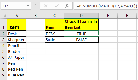
The MATCH function looks for an exact match of value in cell C2 in range A2:A9. Since DESK is on the list, it shows a TRUE value and FALSE for SCALE.

So yeah, these are the ways, using which you can find if a value is in the list or not and then take action on them as you like using IF function. I explained how to find value in a range in the best way possible. Let me know if you have any thoughts. The comments section is all yours.

Related Articles:

How to Check If Cell Contains Specific Text in Excel

How to Check A list of Texts In String in Excel

How to take the Average Difference between lists in Excel

How to Get Every Nth Value From A list in Excel

Popular Articles:

50 Excel Shortcuts to Increase Your Productivity

How to use the VLOOKUP Function in Excel

How to use the COUNTIF function in Excel

How to use the SUMIF Function in Excel

Источник

What is IFERROR Function in Excel?

The IFERROR function in Excel checks a formula (or a cell) for errors and returns a specified value in place of the error. This returned value can be a text message, an empty string, a logical value, a number, etc. The errors handled by the function include “#N/A,” “#DIV/0!,” “#NAME?,” and so on.

For example, cells A1, A2, and A3 contain the numbers 24, 35, and 78 respectively. We perform the following tasks in the given sequence:

To find the minimum number among the listed ones, we enter the formula “=MN(A1:A3)” in cell A4. It returns the “#NAME?” error because the correct function is MIN.
To return a custom message, we enter the formula “=IFERROR(MN(A1:A3),”incorrect function name”)” in cell A4. It returns the text “incorrect function name” (without the double quotation marks).

In this way, the IFERROR excel function replaces the error message (#NAME?) with a customized text string (incorrect function name).

In Excel, errors are displayed on account of multiple reasons. The IFERROR function detects and deals with these errors the way the user wants.

The purpose of using the IFERROR function is to return a customized and specified result in case a formula evaluates to an error. However, if no error is detected, the function returns the output of the formula.

The IFERROR function is categorized under the Logical functions of Excel.

What is IFERROR Function in Excel?
Syntax
- How to Use IFERROR Excel?
  - #1–“#N/A” Error
  - #2–“#DIV/0!” Error
  - #3–“#NAME?” Error
  - #4–“#NULL!” Error
  - #5–“#NUM!” Error
  - #6–“#REF!” Error
  - #7–“#VALUE!” Error
- Frequently Asked Questions
- Recommended Articles

Syntax

The syntax of the IFERROR excel function is shown in the following image:

The function accepts the following arguments:

Value: This is the value to be checked for errors. It can be a cell reference, formula, value or expression.
Value_if_error: This is the output returned in case an error is found. It can be a text string, blank cell, number, logical value, and so on.

Both the preceding arguments are mandatory.

How to Use IFERROR Excel?

Let us go through some examples to understand how the IFERROR function handles the Excel errorsErrors in excel are common and often occur at times of applying formulas. The list of nine most common excel errors are — #DIV/0, #N/A, #NAME?, #NULL!, #NUM!, #REF!, #VALUE!, #####, Circular Reference.read more. Every example covers one Excel error.

You can download this IFERROR Function Excel Template here – IFERROR Function Excel Template

#1–“#N/A” Error

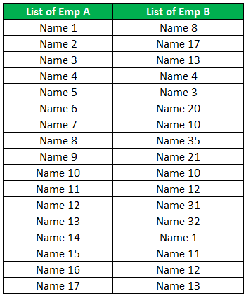
The following table shows the names of some employees segregated in two columns titled “list of emp A” and “list of emp B.” Every name is written as “name” followed by a number. Some names are common to both the columns, while some are present in just one column.

We want to create an excel listA list can be created in Excel to define a list of items/values as predefined values. It may be created using the Data Validation tool so that users may select from a list rather than entering their own values.read more that separates the common names (present in both the columns) from those absent in the first column (list of emp A). Use the following functions:

The VLOOKUPThe VLOOKUP excel function searches for a particular value and returns a corresponding match based on a unique identifier. A unique identifier is uniquely associated with all the records of the database. For instance, employee ID, student roll number, customer contact number, seller email address, etc., are unique identifiers.
read more function of Excel must look up values in the first column (list of emp A).
The IFERROR function of Excel must return the text string “name not in list A” for all “#N/A” errors.

The steps to apply the VLOOKUP and IFERROR functions (with reference to the current example) are listed as follows:

Step 1: Enter the following VLOOKUP formula in cell C2.

“=VLOOKUP(B2,$A:$A,1,0)”

Press the “Enter” key. Drag the formula downwards till the cell C18. The output of the VLOOKUP formula is shown in column C of the following image.

The VLOOKUP formula looks for a name of column B in column A. It returns the “#N/A” error (in column C) for the names that are absent in column A. Such names could not be found in column A as they are present only in column B.

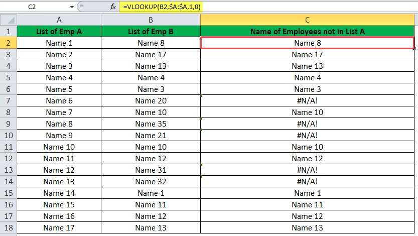
Step 2: Replace the “#N/A” errors (shown in column C of the preceding image) with the text string “name not in list A.” For this, enter the following formula in cell C2.

“=IFERROR(VLOOKUP(B2,$A:$A,1,0),”Name not in list A”)”

Press the “Enter” key. Drag the IFERROR formula till cell C18.

For the ease of understanding, we have displayed the formulas of column C in the succeeding image. Some cells of column C are shown in green. These are the ones that had returned the “#N/A” error in the preceding step (step 1).

The formula “VLOOKUP(B2,$A:$A,1,0)” becomes the first argument and the string “name not in list A” becomes the second argument of the IFERROR function.

The IFERROR function checks the first argument for an error. If the VLOOKUP formula evaluates to an error, the second argument of the IFERROR function is returned. It has already been stated that the VLOOKUP formula evaluates to an error if the lookup value is not found in column A.

Step 3: The output of the IFERROR formula appears in column C, as shown in the succeeding image.

The IFERROR function returns the name if the VLOOKUP formula does not evaluate to an error. However, if the VLOOKUP formula does evaluate to an error, the IFERROR function returns the string “name not in list A.”

In this way, all the “#N/A” errors have been replaced by the text string “name not in list A.” This string implies that the particular name is not in list A (column A).

Hence, “name 20,” “name 35,” “name 21,” “name 31,” and “name 32” are present in column B but not in column A. The names common to both the columns (shown without color) have been separated (in column C) from those absent in column A (shown in green).

#2–“#DIV/0!” Error

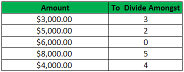
The following table shows some amounts (in $) in the first column titled “amount.” We want to distribute every amount equally among the corresponding number of people mentioned in the second column named “to divide amongst.”

Use the following formulas or functions:

The division formula must divide the amounts among the stated number of people.
The IFERROR function must return the text string “no of person < 1” for all “#DIV/0!” errors.

The steps to apply the division formula and the IFERROR function are listed as follows:

Step 1: Enter the following division formula in cell C2.

“=amount/number of people” or “A2/B2”

Press the “Enter” key. Drag the formula downwards till cell C6. The output of the division formula is shown in column C of the following image.

Cell C4 shows the “#DIV/0!” error because the number of people (in cell B4), i.e., the denominator is zero.

Note: In Excel, any number divided by zero returns the “#DIV/0!” error.

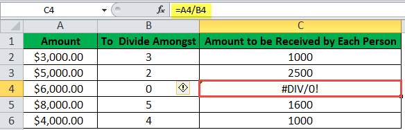
Step 2: To replace the “#DIV/0!” error with the text string “no of person < 1,” enter the following formula in cell C2.

“=IFERROR((A2/B2),”No of Person < 1″)”

Press the “Enter” key. Drag the formula till cell C6. The output appears in column C, as shown in the following image.

In cases where the argument “A2/B2” does not evaluate to an error, the IFERROR formula returns the amount (in column C). Wherever the first argument (A2/B2) evaluates to an error, the text string “no of person < 1” is returned. This text string (in cell C4) implies that the number of persons among which $6,000 is to be divided is less than 1.

Hence, the amounts listed in column A have been divided among the number of people stated in column B. The amount received by each person is stated in column C.

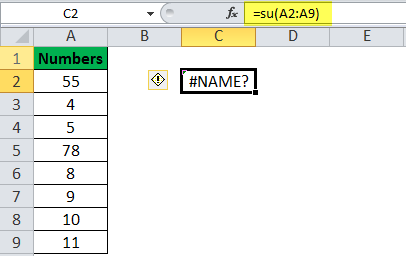
#3–“#NAME?” Error

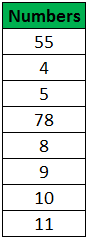
The following list shows some numbers to be added. Use the following functions:

The SUM function in ExcelThe SUM function in excel adds the numerical values in a range of cells. Being categorized under the Math and Trigonometry function, it is entered by typing “=SUM” followed by the values to be summed. The values supplied to the function can be numbers, cell references or ranges.read more must sum the given numbers.
The IFERROR function of Excel must return the text string “typed wrong formula” for all “#NAME?” errors.

The steps to apply the SUM and the IFERROR function are listed as follows:

Step 1: Enter the following formula in cell C2.

“=SU(A2:A9)”

The same is shown in the succeeding image.

Press the “Enter” key. The “#NAME?” error appears in cell C2. This is because we have mistakenly entered the function name as “SU” instead of “SUM.”

Step 2: To replace the “#NAME?” error with the text string “typed wrong formula,” enter the following formula in cell C2.

“=IFERROR(SU(A2:A9),”Typed Wrong Formula”)”

Press the “Enter” key. The formula is shown in the following image.

Step 3: The output appears in cell C2 of the following image. Hence, the IFERROR function has returned the text string “typed wrong formula” in cell C2. This string implies that the name of the function (SUM) has been typed incorrectly.

The given text string is returned because there is an error in the first argument [SU(A2:A9)] of the IFERROR function. Had we entered the correct function name (SUM), the output of the IFERROR formula (in cell C2) would have been the sum of the listed numbers, i.e., 180.

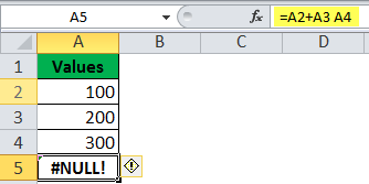
#4–“#NULL!” Error

The following list shows three numbers in the range A2:A4. We want to sum the numbers using the following formulas or functions:

The arithmetic operator “plus” (+) must be used to add the numbers in cells A2, A3, and A4.
The IFERROR function must return the total of the listed numbers.

The steps to use the plus sign (+) and the IFERROR function are listed as follows:

Step 1: Enter the following formula in cell A5.

“=A2+A3 A4”

Press the “Enter” key. The “#NULL!” error appears in cell A5, as shown in the following image. This error appears because we have forgotten to enter the relevant arithmetic operator before the reference A4. Rather, we have mistakenly entered a space before A4.

Step 2: To replace the “#NULL!” error with the total of the listed numbers in column A, enter the following formula in cell A5.

“=IFERROR((A2+A3 A4),(SUM(A2:A4)))”

Press the “Enter” key.

The first argument, “A2+A3 A4,” is checked for an error. The second argument, “SUM(A2:A4),” is the “value_if_error.” This implies that if the first argument evaluates to an error, the function returns the output of the second argument “SUM(A2:A4).”

Hence, the IFERROR formula returns the sum 600 in cell A5, as shown in the following image.

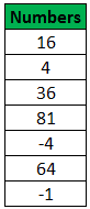
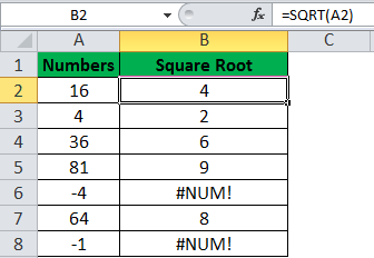
#5–“#NUM!” Error

The following list shows some numbers. We want to find the square roots of these numbers. Use the following functions:

The SQRT function in Excel must calculate the square roots of the given numbers.
The IFERROR function must return the text string “a negative number” for all “#NUM!” errors.

The steps to apply the SQRT FunctionThe Square Root function is an arithmetic function built into Excel that is used to determine the square root of a given number. To use this function, type the term =SQRT and hit the tab key, which will bring up the SQRT function. Moreover, this function accepts a single argument.read more and the IFERROR functions are listed as follows:

Step 1: Enter the following SQRT formula in cell B2.

“=SQRT(A2)”

Press the “Enter” key. Drag the formula downwards till cell B8. The output of the SQRT function is shown in column B of the following image.

The SQRT function helps calculate the square root of a number. However, the square root of a negative number does not exist. So, the SQRT function returns “#NUM!” errors for such numbers.

Step 2: To replace the “#NUM!” errors with the text string “a negative number,” enter the following formula in cell B2.

“=IFERROR(SQRT(A2),”A Negative Number”)”

Press the “Enter” key. Drag the formula till cell B8. The output of the formula is shown in column B of the following image.

The IFERROR function returns the result of the SQRT formula for all positive numbers. For the negative numbers, the IFERROR function returns the text “a negative number.” This text string notifies the user that the number whose square root needs to be found is negative.

Hence, the square roots of the listed numbers have been calculated and the resulting “#NUM!” errors have been replaced with a custom message (a negative number).

#6–“#REF!” Error

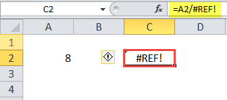
The following image shows two numbers in cells A2 and A3. These numbers have been divided with the help of the formula (=A2/A3) entered in cell C2. We want to delete row 3. Use the following techniques and functions:

The row 3 must be deleted by right-clicking its header and choosing “delete.”
The IFERROR function of Excel must return the text string “reference deleted” for the “#REF!” errors.

The steps to delete row 3 and apply the IFERROR function are listed as follows:

Step 1: Select row 3 by clicking the header (3) appearing on the leftmost side of the Excel sheet. Right-click the selection and choose “delete” from the context menu.

The row 3 is deleted and the “#REF!” error appears in cell C2, as shown in the following image.

The cell A3 was a part of the formula entered in cell C2. Since Excel is unable to locate the value (or cell reference) of the denominator, it returns the “#REF!” error in cell C2.

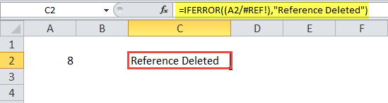
Step 2: To replace the “#REF!” error with the string “reference deleted,” enter the following formula in cell C2.

“=IFERROR((A2/#REF!),”Reference Deleted”)”

Press the “Enter” key. The output of the IFERROR formula appears in cell C2 of the following image.

The IFERROR function checks whether the first argument (A2/#REF!) evaluates to an error or not. Since it does return an error, the function returns the second argument (reference deleted) as the output.

The text string “reference deleted” implies that the cell referenceCell reference in excel is referring the other cells to a cell to use its values or properties. For instance, if we have data in cell A2 and want to use that in cell A1, use =A2 in cell A1, and this will copy the A2 value in A1.read more entered in the division formula has been deleted. This text string is the argument “value_if_error.”

Hence, row 3 has been deleted and the resulting “#REF!” error has been replaced by the string “reference deleted.”

#7–“#VALUE!” Error

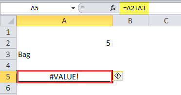
The following image shows two values in cells A2 and A3. We want to add these values. Use the following formulas or functions:

The arithmetic operator plus (+) must sum up the given values.
The IFERROR function must return the text string “text can’t add to number” for the “#VALUE!” errors.

The steps to use the plus symbol (+) and the IFERROR function are listed as follows:

Step 1: Enter the following formula in cell A5.

“=A2+A3”

Press the “Enter” key. The “#VALUE!” error appears in cell A5. This is because cell A2 contains a number while A3 contains a text string. The addition of a numeric and text value has resulted in an error. The same is shown in the following image.

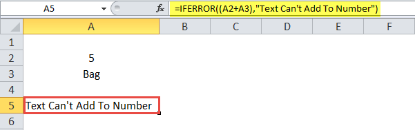
Step 2: To replace the “#VALUE!” error with the text string “text can’t add to number,” enter the following formula in cell A5.

“=IFERROR((A2+A3),”Text Can’t Add to Number”)”

Press the “Enter” key. The output of the IFERROR formula is shown in cell A5 of the following image.

The IFERROR function checks the first argument (A2+A3) for an error. Since this argument does evaluate to an error, the function returns the second argument (text can’t add to number). The text string “text can’t add to number” implies that a text value cannot be added to a numeric value.

Had there been a number in place of the string “bag,” the IFERROR function would have returned the sum of the two numbers.

Hence, since the given values could not be added, the resulting “#VALUE!” error has been replaced by a custom message (text can’t add to number).

Likewise, the IFERROR function can be used for managing errors in Excel. Moreover, the output to be returned (in case of an error) can be customized as per the requirements of the user.

Frequently Asked Questions

1. Define the IFERROR function of Excel.

The IFERROR function detects and handles the various types of Excel errors like “#N/A,” “#DIV/0!,” “#REF!,” “#VALUE!,” and so on. In place of these errors, the function returns a text message, number, empty string, logical value, etc.

The syntax of the IFERROR function of Excel is stated as follows:

“IFERROR(value,value_if_error)”

The first argument “value” is checked for errors. The second argument, “value_if_error,” is returned in case an error is found in the first argument. Both the arguments of the IFERROR function are mandatory.

2. When is the IFERROR function used and how does it work in Excel?

The IFERROR function is used in the following situations:

a. To capture the error and notify its presence to the user
b. To tell Excel what is to be done in case the first argument runs into an error
c. To replace the error with a customized message

The IFERROR function works as follows:

a. The function checks the first argument for errors.
b. In case the first argument does evaluate to an error, the function returns a predefined response. This response is entered as the second argument in the function.
c. In case the first argument does not run into an error, the function returns the result of the first argument.

3. How does the IFERROR function return a blank cell in Excel?

To return a blank cell, an empty string needs to be entered in the second argument of the IFERROR function. For example, two cells contain the following values:

• Cell A1 contains 20
• Cell A2 contains 0

Enter the formula “=IFERROR(A1/A2,””) in cell B1. After pressing the “Enter” key, it returns an empty cell (B1).

As long as cell A2 contains zero, the given IFERROR formula returns a blank cell. This is because the formula identifies division by zero as an error. The moment a value is entered in cell A2, the IFERROR formula returns the result of A1/A2.

Had A1 been a blank cell and A2 contained 20, the formula “=IFERROR(A1/A2,“no message”) would have returned 0. This is because the formula does not identify a blank cell in the numerator as an error. Hence, it returns the result of the first argument.

NOT in Excel

NOT function is an inbuilt function that is categorized under the Logical Function; the logical function operates under a logical test. It is also called Boolean logic or function. Boolean functions are most commonly used along with or in conjunction with other functions, specifically along with conditional test functions (“IF’’ FUNCTION), to create formulas that can evaluate multiple parameters or criteria and produce desired results depending on that criteria. It is used as an individual function or part of the formula and other excel functions in a cell. E.G. with AND, IF & OR function. It returns the opposite value of a given logical value in the formula, NOT function is used to reverse a logical value. If the argument is FALSE, then TRUE is returned and vice versa.

Note: Use NOT function when you want to make sure a value is not equal to one Specific or particular value

It’s a worksheet function; it is also used as part of the formula in a cell along with other excel function

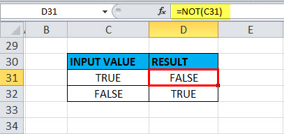
If given with the value TRUE, the Not function returns FALSE
If given with the value FALSE, the Not function returns TRUE

NOT Formula in Excel

Below is the NOT Formula in excel:

=NOT (logical) logical – A value that can be evaluated to TRUE or FALSE

The only parameter in the NOT function is a logical value.

The logical test or argument can be either entered directly, or it can be entered as a reference to a cell that contains a logical value, and it always returns the Boolean value (“TRUE” OR “FALSE”) only.

How to Use the NOT Function in Excel?

NOT Function in Excel is very simple and easy to use. Let us now see how to use the NOT function in excel with the help of some examples.

You can download this NOT function Excel Template here – NOT function Excel Template

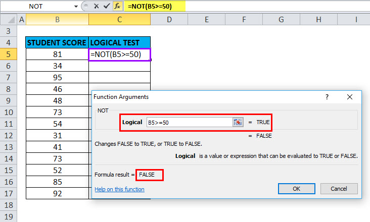
Example #1 – Excel NOT Function

Here a logical test is performed on the given set of values (Student score) by using the NOT function. Here, we will check which value is greater than or equal to 50.

In the table, we have 2 columns, the first column contains student score & the second column is the logical test column, where the NOT function is performed.

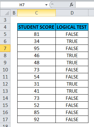
Result: It will return the reverse value if the value is greater than or equal to 50, then it will return FALSE and if the lesser than or equal to 50, it will return TRUE as output.

The result will be as given below:

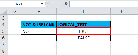
Example #2 – Using NOT Function with ISBLANK

the logical test is performed on the H5 & H6 Cells by using the NOT Function along with ISBLANK function; here will check if cells H5 & H6 is blank OR not using NOT function along with ISBLANK in excel

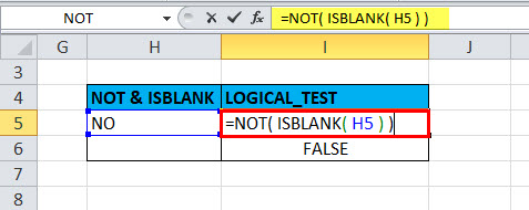
OUTPUT will be TRUE.

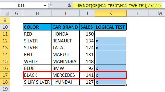
Example #3 – NOT Function along with “IF” and “OR” Function

Here the color check is performed for the cars in the below-mentioned table by using NOT Function along with “if” and “or” function

Here we have to sort out color “WHITE” or “RED” from the given set of data

=IF(NOT(OR(H11=”RED”,H11=”WHITE”)),”x”,””) formula is used

This logical condition is applied on a Color column containing any car with color “RED” or “WHITE”,

if the condition is true, then it will return blank as output,

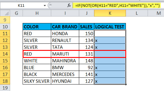
if not true, then it will return x as output

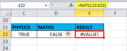
Example #4 – VALUE! Error

It Occurs when the supplied argument is not a logical or numeric value.

Suppose, if we give a range in the logical argument

Selected the range C22:D22 in the logical argument, i.e. =NOT (C22:D22)

a function returns a #VALUE error because the NOT function does not allow any range and can take only a logical test or argument or one condition.

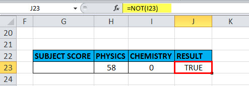
Example #5 – NOT Function for an empty cell or blank or “0”

An empty cell or blank or “0” are treated as false, therefore “NOT” function returns TRUE

Here in the cell “I23”, the stored value is “0” suppose if I apply the “NOT” function with logical argument or value as “0” or “I23”, Output will be TRUE.

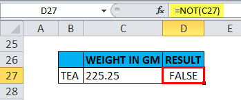
Example #6 – NOT Function for Decimals

When the value is decimal in a cell

Suppose if we take the argument as decimals, i.e. suppose if I apply the “NOT” function with logical argument or value as “225.25” or “c27”, Output will be FALSE.

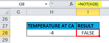
Example #7 – NOT Function for Negative Number

When the value is a negative number in a cell

Suppose if we take the argument as a negative number, i.e. suppose if I apply the “NOT” function with logical argument or value as “-4” or “H27”, Output will be FALSE.

Example #8 – When the value or Reference is Boolean Input in NOT Function

When the value or reference is Boolean input (“TRUE” OR “FALSE”) in a cell.

Here in the cell “C31”, the stored value is “TRUE” suppose if I apply the “NOT” function with logical argument or value as “C31” or “TRUE”, Output will be FALSE. It will be vice versa if the logical argument is “FALSE”, i.e. the NOT function returns the “TRUE” value as output.

What’s on this page

Check if the cell contains any value in the list
Display matches if cell contains text from list (Excel 2019)
Display matches if cell contains text from list (Earlier Excel versions)
Filter delimited values not in list (Excel 365)

1. Check if the cell contains any value in the list

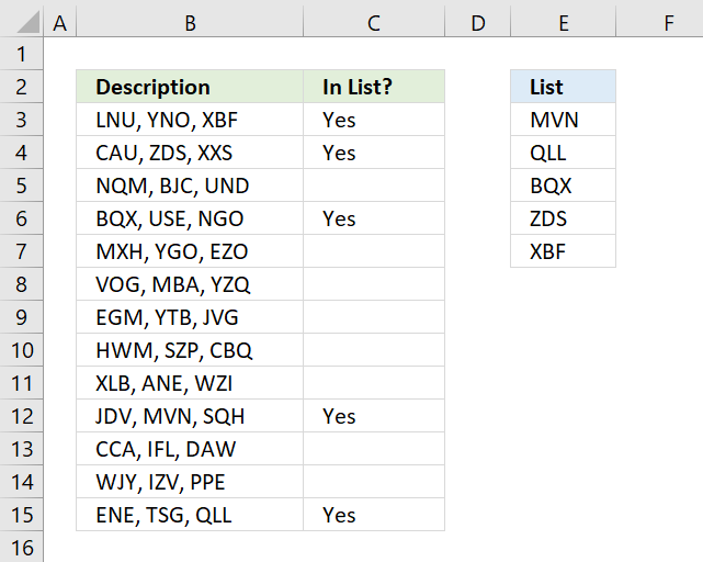
The image above shows an array formula in cell C3 that checks if cell B3 contains at least one of the values in List (E3:E7), it returns «Yes» if any of the values are found in column B and returns nothing if the cell contains none of the values.

For example, cell B3 contains XBF which is found in cell E7. Cell B4 contains text ZDS found in cell E6. Cell C5 contains no values in the list.

=IF(OR(COUNTIF(B3,»*»&$E$3:$E$7&»*»)), «Yes», «»)

You need to enter this formula as an array formula if you are not an Excel 365 subscriber. There is another formula below that doesn’t need to be entered as an array formula, however, it is slightly larger and more complicated.

Type formula in cell C3.
Press and hold CTRL + SHIFT simultaneously.
Press Enter once.
Release all keys.

Excel adds curly brackets to the formula automatically if you successfully entered the array formula. Don’t enter the curly brackets yourself.

1.1 Explaining formula in cell C3

Step 1 — Check if the cell contains any of the values in the list

The COUNTIF function lets you count cells based on a condition, however, it also allows you to count cells based on multiple conditions if you use a cell range instead of a cell.

COUNTIF(range, criteria)

The criteria argument utilizes a beginning and ending asterisk in order to match a text string and not the entire cell value, asterisks are one of two wildcard characters that you are allowed to use.

The ampersands concatenate the asterisks to cell range E3:E7.

COUNTIF(B3,»*»&$E$3:$E$7&»*»)

becomes

COUNTIF(«LNU, YNO, XBF», {«*MVN*»; «*QLL*»; «*BQX*»; «*ZDS*»; «*XBF*»})

and returns this array

{0; 0; 0; 0; 1}

which tells us that the last value in the list is found in cell B3.

Step 2 — Return TRUE if at least one value is 1

The OR function returns TRUE if at least one of the values in the array is TRUE, the numerical equivalent to TRUE is 1.

OR({0; 0; 0; 0; 1})

returns TRUE.

Step 3 — Return Yes or nothing

The IF function then returns «Yes» if the logical test evaluates to TRUE and nothing if the logical test returns FALSE.

IF(TRUE, «Yes», «»)

returns «Yes» in cell B3.

Regular formula

The following formula is quite similar to the formula above except that it is a regular formula and it has an additional INDEX function.

=IF(OR(INDEX(COUNTIF(B3,»*»&$E$3:$E$7&»*»),)), «Yes», «»)

2. Display matches if the cell contains text from a list

The image above demonstrates a formula that checks if a cell contains a value in the list and then returns that value. If multiple values match then all matching values in the list are displayed.

For example, cell B3 contains «ZDS, YNO, XBF» and cell range E3:E7 has two values that match, «ZDS» and «XBF».

Formula in cell C3:

=TEXTJOIN(«, «, TRUE, IF(COUNTIF(B3, «*»&$E$3:$E$7&»*»), $E$3:$E$7, «»))

The TEXTJOIN function is available for Office 2019 and Office 365 subscribers. You will get a #NAME error if your Excel version is missing this function. Office 2019 users may need to enter this formula as an array formula.

The next formula works with most Excel versions.

Array formula in cell C3:

=INDEX($E$3:$E$7, MATCH(1, COUNTIF(B3, «*»&$E$3:$E$7&»*»), 0))

However, it only returns the first match. There is another formula below that returns all matching values, check it out.

How to enter an array formula

2.1 Explaining formula in cell C3

Step 1 — Count cells containing text strings

The COUNTIF function lets you count cells based on a condition, we are going to use multiple conditions. I am going to use asterisks to make the COUNTIF function check for a partial match.

The asterisk is one of two wild card characters that you can use, it matches 0 (zero) to any number of any characters.

COUNTIF(B3, «*»&$E$3:$E$7&»*»)

becomes

COUNTIF(«ZDS, YNO, XBF», {«*MVN*»; «*QLL*»; «*BQX*»; «*ZDS*»; «*XBF*»})

and returns {1; 0; 0; 0; 1}.

This array contains as many values as there values in the list, the position of each value in the array matches the position of the value in the list. This means that we can tell from the array that the first value and the last value is found in cell B3.

Step 2 — Return the actual value

The IF function returns one value if the logical test is TRUE and another value if the logical test is FALSE.

IF(logical_test, [value_if_true], [value_if_false])

This allows us to create an array containing values that exists in cell B3.

IF(COUNTIF(B3, «*»&$E$3:$E$7&»*»), $E$3:$E$7, «»)

becomes

IF(COUNTIF(«ZDS, YNO, XBF», {«*MVN*»; «*QLL*»; «*BQX*»; «*ZDS*»; «*XBF*»}), {«*MVN*»; «*QLL*»; «*BQX*»; «*ZDS*»; «*XBF*»}, «»)

and returns {«»;»»;»»;»ZDS»;»XBF»}.

Step 3 — Concatenate values in array

The TEXTJOIN function allows you to combine text strings from multiple cell ranges and also use delimiting characters if you want.

TEXTJOIN(delimiter, ignore_empty, text1, [text2], …)

TEXTJOIN(«, «, TRUE, IF(COUNTIF(B3, «*»&$E$3:$E$7&»*»), $E$3:$E$7, «»))

becomes

TEXTJOIN(«, «, TRUE, {«»;»»;»»;»ZDS»;»XBF»})

and returns text strings ZDS, XBF.

3. Display matches if cell contains text from a list (Earlier Excel versions)

The image above demonstrates a formula that returns multiple matches if the cell contains values from a list. This array formula works with most Excel versions.

Array formula in cell C3:

=IFERROR(INDEX($G$3:$G$7, SMALL(IF(COUNTIF($B3, «*»&$G$3:$G$7&»*»), MATCH(ROW($G$3:$G$7), ROW($G$3:$G$7)), «»), COLUMNS($A$1:A1))), «»)

How to enter an array formula

Copy cell C3 and paste to cell range C3:E15.

3.1 Explaining formula in cell C3

Step 1 — Identify matching values in cell

The COUNTIF function lets you count cells based on a condition, we are going to use a cell range instead. This will return an array of values.

COUNTIF($B3, «*»&$G$3:$G$7&»*»)

becomes

COUNTIF(«ZDS, YNO, XBF», {«*MVN*»; «*QLL*»; «*BQX*»; «*ZDS*»; «*XBF*»})

and returns {0; 0; 0; 1; 1}.

Step 2 — Calculate relative positions of matching values

The IF function returns one value if the logical test is TRUE and another value if the logical test is FALSE.

IF(logical_test, [value_if_true], [value_if_false])

This allows us to create an array containing values representing row numbers.

IF(COUNTIF($B3, «*»&$G$3:$G$7&»*»), MATCH(ROW($G$3:$G$7), ROW($G$3:$G$7)), «»)

becomes

IF({0; 0; 0; 2; 1}, MATCH(ROW($G$3:$G$7), ROW($G$3:$G$7)), «»)

becomes

IF({0; 0; 0; 2; 1}, {1; 2; 3; 4; 5}, «»)

and returns {«»; «»; «»; 4; 5}.

Step 3 — Extract the k-th smallest number

I am going to use the SMALL function to be able to extract one value in each cell in the next step.

SMALL(array, k)

SMALL(IF(COUNTIF($B3, «*»&$G$3:$G$7&»*»), MATCH(ROW($G$3:$G$7), ROW($G$3:$G$7)), «»), COLUMNS($A$1:A1)))

becomes

SMALL({«»; «»; «»; 4; 5}, COLUMNS($A$1:A1)))

The COLUMNS function calculates the number of columns in a cell range, however, the cell reference in our formula grows when you copy the cell and paste to adjacent cells to the right.

SMALL({0; 0; 0; 4; 5}, COLUMNS($A$1:A1)))

becomes

SMALL({«»; «»; «»; 4; 5}, 1)

and returns 4.

Step 4 — Return value based on row number

The INDEX function returns a value from a cell range or array, you specify which value based on a row and column number. Both the [row_num] and [column_num] are optional.

INDEX(array, [row_num], [column_num])

INDEX($G$3:$G$7, SMALL(IF(COUNTIF($B3, «*»&$G$3:$G$7&»*»), MATCH(ROW($G$3:$G$7), ROW($G$3:$G$7)), «»), COLUMNS($A$1:A1)))

becomes

INDEX($G$3:$G$7, 4)

becomes

INDEX({«MVN»;»QLL»;»BQX»;»ZDS»;»XBF»}, 4)

and returns «ZDS» in cell C3.

Step 5 — Remove error values

The IFERROR function lets you catch most errors in Excel formulas except #SPILL! errors. Be careful when using the IFERROR function, it may make it much harder spotting formula errors.

IFERROR(value, value_if_error)

There are two arguments in the IFERROR function. The value argument is returned if it is not evaluating to an error. The value_if_error argument is returned if the value argument returns an error.

IFERROR(INDEX($G$3:$G$7, SMALL(IF(COUNTIF($B3, «*»&$G$3:$G$7&»*»), MATCH(ROW($G$3:$G$7), ROW($G$3:$G$7)), «»), COLUMNS($A$1:A1))), «»)

4. Filter delimited values not in the list (Excel 365)

The formula in cell C3 lists values in cell B3 that are not in the List specified in cell range E3:E7. The formula returns #CALC! error if all values are in the list, see cell C14 as an example.

Excel 365 dynamic array formula in cell C3:

=LET(z,TRIM(TEXTSPLIT(B3,,»,»)),TEXTJOIN(«, «,TRUE,FILTER(z,NOT(COUNTIF($E$3:$E$7,z)))))

4.1 Explaining formula

Step 1 — Split values with a delimiting character

The TEXTSPLIT function splits a string into an array based on delimiting values.

Function syntax: TEXTSPLIT(Input_Text, col_delimiter, [row_delimiter], [Ignore_Empty])

TEXTSPLIT(B3,,»,»)

becomes

TEXTSPLIT(«ZDS, VTO, XBF»,,»,»)

and returns

{«ZDS»; » VTO»; » XBF»}

Step 2 — Remove leading and trailing spaces

The TRIM function deletes all blanks or space characters except single blanks between words in a cell value.

Function syntax: TRIM(text)

TRIM(TEXTSPLIT(B3,,»,»))

becomes

TRIM({«ZDS»; » VTO»; » XBF»})

and returns

{«ZDS»; «VTO»; «XBF»}

Step 3 — Check if values are in list

The COUNTIF function calculates the number of cells that is equal to a condition.

Function syntax: COUNTIF(range, criteria)

COUNTIF($E$3:$E$7,TRIM(TEXTSPLIT(B3,,»,»)))

becomes

COUNTIF({«MVN»;»QLL»;»BQX»;»ZDS»;»XBF»},{«ZDS»; «VTO»; «XBF»})

and returns

{1; 0; 1}

These numbers indicate if a value is found in the list, zero means not in the list and 1 or higher means that the value is in the list at least once.

The number’s position corresponds to the position of the values. {1; 0; 1} — {«ZDS»; «VTO»; «XBF»} meaning «ZDS» and «XBF» are in the list and «VTO» not.

Step 4 — Not

The NOT function returns the boolean opposite to the given argument.

Function syntax: NOT(logical)

NOT(COUNTIF($E$3:$E$7,TRIM(TEXTSPLIT(B3,,»,»))))

becomes

NOT({1; 0; 1})

and returns

{FALSE; TRUE; FALSE}.

0 (zero) is equivalent to FALSE. The boolean opposite is TRUE.

Any other number than 0 (zero) is equivalent to TRUE. The boolean opposite is FALSE.

Step 5 — Filter

The FILTER function extracts values/rows based on a condition or criteria.

Function syntax: FILTER(array, include, [if_empty])

FILTER(TRIM(TEXTSPLIT(B3,,»,»)),NOT(COUNTIF($E$3:$E$7,TRIM(TEXTSPLIT(B3,,»,»)))))

becomes

FILTER({«ZDS»; «VTO»; «XBF»},{FALSE; TRUE; FALSE})

and returns

«VTO».

Step 6 — Join

The TEXTJOIN function combines text strings from multiple cell ranges.

Function syntax: TEXTJOIN(delimiter, ignore_empty, text1, [text2], …)

TEXTJOIN(«, «,TRUE,FILTER(TRIM(TEXTSPLIT(B3,,»,»)),NOT(COUNTIF($E$3:$E$7,TRIM(TEXTSPLIT(B3,,»,»))))))

becomes

TEXTJOIN(«, «,TRUE,{«VTO»})

and returns

«VTO».

Step 7 — Shorten the formula

The LET function lets you name intermediate calculation results which can shorten formulas considerably and improve performance.

Function syntax: LET(name1, name_value1, calculation_or_name2, [name_value2, calculation_or_name3…])

TEXTJOIN(«, «,TRUE,FILTER(TRIM(TEXTSPLIT(B3,,»,»)),NOT(COUNTIF($E$3:$E$7,TRIM(TEXTSPLIT(B3,,»,»))))))

z — TRIM(TEXTSPLIT(B3,,»,»))

LET(z,TRIM(TEXTSPLIT(B3,,»,»)),TEXTJOIN(«, «,TRUE,FILTER(z,NOT(COUNTIF($E$3:$E$7,z)))))

Источник

This formula relies on the FILTER function to retrieve data based on a logical test built with the COUNTIF function:

=FILTER(list1,COUNTIF(list2,list1))

working from the inside out, the COUNTIF function is used to create the actual filter:

COUNTIF(list2,list1)

Notice we are using list2 as the range argument, and list1 as the criteria argument. In other words, we are asking COUNTIF to count all values in list1 that appear in list2. Because we are giving COUNTIF multiple values for criteria, we get back an array with multiple results:

{1;1;0;1;0;1;0;0;1;0;1;1}

Note the array contains 12 counts, one for each value in list1. A zero value indicates a value in list1 that is not found in list2. Any other positive number indicates a value in list1 that is found in list2. This array is returned directly to the FILTER function as the include argument:

=FILTER(list1,{1;1;0;1;0;1;0;0;1;0;1;1})

The FILTER function uses the array as a filter. Any value in list1 associated with a zero is removed, while any value associated with a positive number survives.

The result is an array of 7 matching values which spill into the range F5:F11. If data changes, FILTER will recalculate and return a new list of matching values based on the new data.

Non-matching values

To extract non-matching values from list1 (i.e. values in list1 that don’t appear in list2) you can add the NOT function to the formula like this:

=FILTER(list1,NOT(COUNTIF(list2,list1)))

The NOT function effectively reverses the result from COUNTIF – any non-zero number becomes FALSE, and any zero value becomes TRUE. The result is a list of the values in list1 that are not present in list2.

With INDEX

It is possible to create a formula to extract matching values without the FILTER function, but the formula is more complex. One option is to use the INDEX function in a formula like this:

The formula in G5, copied down is:

=IFERROR(INDEX(list1,SMALL(IF(COUNTIF(list2,list1),ROW(list1)-ROW(INDEX(list1,1,1))+1),ROWS($F$5:F5))),"")

Note: this is an array formula and must be entered with control + shift + enter, except in Excel 365.

The core of this formula is the INDEX function, which receives list1 as the array argument. Most of the remaining formula simply calculates the row number to use for matching values. This expression generates a list of relative row numbers:

ROW(list1)-ROW(INDEX(list1,1,1))+1

which returns an array of 12 numbers representing the rows in list1:

{1;2;3;4;5;6;7;8;9;10;11;12}

These are filtered with the IF function and the same logic used above in FILTER, based on the COUNTIF function:

COUNTIF(list2,list1) // find matching values

The resulting array looks like this:

{1;2;FALSE;4;FALSE;6;FALSE;FALSE;9;FALSE;11;12} // result from IF

This array is delivered directly to the SMALL function, which is used to fetch the next matching row number as the formula is copied down the column. The k value for SMALL (think nth) is calculated with an expanding range:

ROWS($G$5:G5) // incrementing value for k

The IFERROR function is used to trap errors that occur when the formula is copied down and runs out of matching values. For another example of this idea, see this formula.

Источник

Функция NOT (НЕ) в Excel используется для изменения логического выражения TRUE (Истина) / FALSE (Ложь).

Содержание

Что возвращает функция
Синтаксис
Аргументы функции
Дополнительная информация
Примеры использования функции NOT (НЕ) в Excel
Пример 1. Конвертируем значение TRUE (Истина) в FALSE (Ложь), и наоборот.
Пример 2. Используем функцию NOT (НЕ) с результатом формулы
Пример 3. Используем функцию NOT (НЕ) с числовыми значениями

Что возвращает функция

Логический аргумент, который является обратным логическому аргументу, используемому в функции NOT. Например, =NOT(TRUE) возвращает FALSE (Ложь) и =NOT(FALSE) возвращает TRUE(Истина).

Синтаксис

=NOT (logical) — английская версия

=НЕ(логическое_значение) — русская версия

Аргументы функции

logical (логическое значение) — значение или выражение, которое может быть логически оценено как TRUE (Истина) или FALSE (Ложь)

Дополнительная информация

С помощью функции NOT (НЕ) в Excel вы можете проверить выражение, которое принимает значение TRUE или FALSE. Например, =NOT(1 + 1 = 2) вернет FALSE.

Больше лайфхаков в нашем Telegram Подписаться

Примеры использования функции NOT (НЕ) в Excel

Пример 1. Конвертируем значение TRUE (Истина) в FALSE (Ложь), и наоборот.

Функция преобразует TRUE (Истина) в FALSE (Ложь) и FALSE (Ложь) в TRUE (Истина). Аргумент внутри функции также может быть результатом другой функции, результатом которой являются TRUE / FALSE.

Пример 2. Используем функцию NOT (НЕ) с результатом формулы

Если вы используете функцию с результатом какой-либо формулы (которая возвращает значения TRUE или FALSE), то она конвертирует результат TRUE в FALSE и наоборот. На примере выше, значение в ячейке А2 сравнивается с числом. По результату вычисления, при совпадении условий формулы, NOT (НЕ) выдаст FALSE, или отразит TRUE, если значение не совпадает с условиями.

Пример 3. Используем функцию NOT (НЕ) с числовыми значениями

В Excel, по умолчанию принято, что цифровое значение “0” (ноль) принимается за FALSE, а любое положительное значение — TRUE. Функция NOT (НЕ) при использовании с числами конвертирует “0” (ноль) в TRUE (Истина) и любое позитивное значение или отрицательное в FALSE (Ложь).

Источник

Date yes Add (Subtract) Days to a Date Concatenate Dates Convert Date to Number Convert Date to Text Month Name to Number Create Date Range from Dates Day Number of Year Month Name from Date First Day of Month Add (Subtract) Weeks to a Date If Functions with Dates Max Date Number of Days Between Dates Number of Days in a Month Number of Weeks Between Dates Number of Years Between Dates Split Date & Time into Separate Cells Countdown Remaining Days Insert Dates Random Date Generator Using Dynamic Ranges — Year to Date Values Add (Subtract) Years to a Date Date Formula Examples Extract Day from Date Get Day Name from Date Count Days Left in Month / Year Count Workdays Left in Month / Year Get Last Day of Month Last Business Day of Month / Year Number of Work / Business Days in Month Weekday Abbreviations Auto Populate Dates Number of Months Between Dates Quarter from a Date Years of Service Change Date Format Compare Dates Time yes Add (Subtract) Hours to Time Add (Subtract) Minutes to Time Add (Subtract) Seconds to Time Add Up time (Total Time) Time Differences Change Time Format Convert Minutes to Hours Convert Time to Decimal Convert Time to Hours Convert Time to Minutes Convert Time to Seconds Military Time Round Time to Nearest 15 Minutes Overtime Calculator Number of Hours Between Times Convert Seconds to Minutes, Hours, or Time Count Hours Worked Time Differences Time Format — Show Minutes Seconds Text yes Add Commas to Cells Get First Word from Text Capitalize First Letter Clean & Format Phone #s Remove Extra Trailing / Leading Spaces Add Spaces to Cell Assign Number Value to Text Combine Cells with Comma Combine First and Last Names Convert Text String to Date Convert Text to Number Extract Text From Cell Get Last Word Remove Unwated Characters Extract Text Before or After Character How to Split Text String by Space, Comma, & More Remove Special Characters Remove First Characters from Left Substitute Multiple Values Switch First & Last Names w/ Commas Remove Specific Text from a Cell Extract Text Between Characters (Ex. Parenthesis) Add Leading Zeros to a Number Remove Line Breaks from Text Remove all Numbers from Text Reverse Text Remove Non-Numeric Characters Remove Last Character(s) From Right Separate First and Last Names Separate Text & Numbers Round yes Round Formulas Round Price to Nearest Dollar or Cent Round to Nearest 10, 100, or 1000 Round to Nearest 5 or .5 Round Percentages Round to Significant Figures Count yes Count Blank and Non-blank Cells Count Cells Between Two Numbers Count Cells not Equal to Count if Cells are in Range Count Times Word Appears in Cell Count Words in Cell Count Specific Characters in Column Count Total Number of Characters in Column Count Cells that Equal one of two Results Count Cells that do not Contain Count Cells that Contain Specific Text Count Unique Values in Range Countif — Multiple Criteria Count Total Number of Cells in Range Count Cells with Any Text Count Total Cells in a Table Lookup yes Two Dimensional VLOOKUP VLOOKUP Simple Example Vlookup — Multiple Matches Case Sensitive Lookup Case Sensitive VLOOKUP Sum if — VLOOKUP Case Sensitive Lookup Case Sensitive VLOOKUP Find Duplicates w/ VLOOKUP or MATCH INDEX MATCH MATCH Lookup — Return Cell Address (Not Value) Lookup Last Value in Column or Row Reverse VLOOKUP (Right to Left) Risk Score Bucket with VLOOKUP Sum with a VLOOKUP Function VLOOKUP & INDIRECT VLOOKUP Concatenate VLOOKUP Contains (Partial Match) 17 Reasons Why Your XLOOKUP is Not Working Double (Nested) XLOOKUP — Dynamic Columns IFERROR (& IFNA) XLOOKUP Lookup Min / Max Value Nested VLOOKUP Top 11 Alternatives to VLOOKUP (Updated 2022!) VLOOKUP – Dynamic Column Reference VLOOKUP – Fix #N/A Error VLOOKUP – Multiple Sheets at Once VLOOKUP & HLOOKUP Combined VLOOKUP & MATCH Combined VLOOKUP Between Worksheets or Spreadsheets VLOOKUP Duplicate Values VLOOKUP Letter Grades VLOOKUP Return Multiple Columns VLOOKUP Returns 0? Return Blank Instead VLOOKUP w/o #N/A Error XLOOKUP Multiple Sheets at Once XLOOKUP Between Worksheets or Spreadsheets XLOOKUP by Date XLOOKUP Duplicate Values XLOOKUP Multiple Criteria XLOOKUP Return Multiple Columns XLOOKUP Returns 0? Return Blank Instead XLOOKUP Text XLOOKUP with IF XLOOKUP With If Statement Misc. yes Sort Multiple Columns Use Cell Value in Formula Percentage Change Between Numbers Percentage Breakdown Rank Values Add Spaces to Cell CAGR Formula Average Time Decimal Part of Number Integer Part of a Number Compare Items in a List Dealing with NA() Errors Get Worksheet Name Wildcard Characters Hyperlink to Current Folder Compound Interest Formula Percentage Increase Create Random Groups Sort with the Small and Large Functions Non-volatile Function Alternatives Decrease a Number by a Percentage Calculate Percent Variance Profit Margin Calculator Convert Column Number to Letter Get Full Address of Named Range Insert File Name Insert Path Latitute / Longitude Functions Replace Negative Values Reverse List Range Convert State Name to Abbreviation Create Dynamic Hyperlinks Custom Sort List with Formula Data Validation — Custom Formulas Dynamic Sheet Reference (INDIRECT) Reference Cell in Another Sheet or Workbook Get Cell Value by Address Get Worksheet Name Increment Cell Reference List Sheet Names List Skipped Numbers in Sequence Return Address of Max Value in Range Search by Keywords Select Every Other (or Every nth) Row Basics yes Cell Reference Basics — A1, R1C1, 3d, etc. Add Up (Sum) Entire Column or Row Into to Dynamic Array Formulas Conversions yes Convert Time Zones Convert Celsius to Fahrenheit Convert Pounds to Kilograms Convert Time to Unix Time Convert Feet to Meters Convert Centimeters to Inches Convert Kilometers to Miles Convert Inches to Feet Convert Date to Julian Format Convert Column Letter to Number Tests yes Test if a Range Contains any Text Test if any Cell in Range is Number Test if a Cell Contains a Specific Value Test if Cell Contains Any Number Test if Cell Contains Specific Number Test if Cell is Number or Text If yes Percentile If Subtotal If Sumproduct If Large If and Small If Median If Concatentate If Max If Rank If TEXTJOIN If Sum yes Sum if — Begins With / Ends With Sum if — Month or Year to Date Sum if — By Year Sum if — Blank / Non-Blank Sum if — Horizontal Sum Count / Sum If — Cell Color INDIRECT Sum Sum If — Across Multiple Sheets Sum If — By Month Sum If — Cells Not Equal To Sum If — Not Blank Sum if — Between Values Sum If — Week Number Sum Text Sum if — By Category or Group Sum if — Cell Contains Specific Text (Wildcards) Sum if — Date Rnage Sum if — Dates Equal Sum if — Day of Week Sum if — Greater Than Sum if — Less Than Average yes Average Non-Zero Values Average If — Not Blank Average — Ignore 0 Average — Ignore Errors Math yes Multiplication Table Cube Roots nth Roots Square Numbers Square Roots Calculations yes Calculate a Ratio Calculate Age KILLLLLLL Calculate Loan Payments GPA Formula Calculate VAT Tax How to Grade Formulas Find yes Find a Number in a Column / Workbook Find Most Frequent Numbers Find Smallest n Values Find nth Occurance of Character in Text Find and Extract Number from String Find Earliest or Latest Date Based on Criteria Find First Cell with Any Value Find Last Row Find Last Row with Data Find Missing Values Find Largest n Values Most Frequent Number Conditional Formatting yes Conditional Format — Dates & Times Conditional Format — Highlight Blank Cells New Functions XLOOKUP Replaces VLOOKUP, HLOOKUP, and INDEX / MATCH Logical yes AND Checks whether all conditions are met. TRUE/FALSE IF If condition is met, do something, if not, do something else. IFERROR If result is an error then do something else. NOT Changes TRUE to FALSE and FALSE to TRUE. OR Checks whether any conditions are met. TRUE/FALSE XOR Checks whether one and only one condition is met. TRUE/FALSE Lookup & Reference yes FALSE The logical value: FALSE. TRUE The logical value: TRUE. ADDRESS Returns a cell address as text. AREAS Returns the number of areas in a reference. CHOOSE Chooses a value from a list based on it’s position number. COLUMN Returns the column number of a cell reference. COLUMNS Returns the number of columns in an array. HLOOKUP Lookup a value in the first row and return a value. HYPERLINK Creates a clickable link. INDEX Returns a value based on it’s column and row numbers. INDIRECT Creates a cell reference from text. LOOKUP Looks up values either horizontally or vertically. MATCH Searches for a value in a list and returns its position. OFFSET Creates a reference offset from a starting point. ROW Returns the row number of a cell reference. ROWS Returns the number of rows in an array. TRANSPOSE Flips the oriention of a range of cells. VLOOKUP Lookup a value in the first column and return a value. Date & Time yes DATE Returns a date from year, month, and day. DATEDIF Number of days, months or years between two dates. DATEVALUE Converts a date stored as text into a valid date DAY Returns the day as a number (1-31). DAYS Returns the number of days between two dates. DAYS360 Returns days between 2 dates in a 360 day year. EDATE Returns a date, n months away from a start date. EOMONTH Returns the last day of the month, n months away date. HOUR Returns the hour as a number (0-23). MINUTE Returns the minute as a number (0-59). MONTH Returns the month as a number (1-12). NETWORKDAYS Number of working days between 2 dates. NETWORKDAYS.INTL Working days between 2 dates, custom weekends. NOW Returns the current date and time. SECOND Returns the second as a number (0-59) TIME Returns the time from a hour, minute, and second. TIMEVALUE Converts a time stored as text into a valid time. TODAY Returns the current date. WEEKDAY Returns the day of the week as a number (1-7). WEEKNUM Returns the week number in a year (1-52). WORKDAY The date n working days from a date. WORKDAY.INTL The date n working days from a date, custom weekends. YEAR Returns the year. YEARFRAC Returns the fraction of a year between 2 dates. Engineering yes CONVERT Convert number from one unit to another. Financial yes FV Calculates the future value. PV Calculates the present value. NPER Calculates the total number of payment periods. PMT Calculates the payment amount. RATE Calculates the interest Rate. NPV Calculates the net present value. IRR The internal rate of return for a set of periodic CFs. XIRR The internal rate of return for a set of non-periodic CFs. PRICE Calculates the price of a bond. YIELD Calculates the bond yield. INTRATE The interest rate of a fully invested security. Information yes CELL Returns information about a cell. ERROR.TYPE Returns a value representing the cell error. ISBLANK Test if cell is blank. TRUE/FALSE ISERR Test if cell value is an error, ignores #N/A. TRUE/FALSE ISERROR Test if cell value is an error. TRUE/FALSE ISEVEN Test if cell value is even. TRUE/FALSE ISFORMULA Test if cell is a formula. TRUE/FALSE ISLOGICAL Test if cell is logical (TRUE or FALSE). TRUE/FALSE ISNA Test if cell value is #N/A. TRUE/FALSE ISNONTEXT Test if cell is not text (blank cells are not text). TRUE/FALSE ISNUMBER Test if cell is a number. TRUE/FALSE ISODD Test if cell value is odd. TRUE/FALSE ISREF Test if cell value is a reference. TRUE/FALSE ISTEXT Test if cell is text. TRUE/FALSE N Converts a value to a number. NA Returns the error: #N/A. TYPE Returns the type of value in a cell. Math yes ABS Calculates the absolute value of a number. AGGREGATE Define and perform calculations for a database or a list. CEILING Rounds a number up, to the nearest specified multiple. COS Returns the cosine of an angle. DEGREES Converts radians to degrees. DSUM Sums database records that meet certain criteria. EVEN Rounds to the nearest even integer. EXP Calculates the exponential value for a given number. FACT Returns the factorial. FLOOR Rounds a number down, to the nearest specified multiple. GCD Returns the greatest common divisor. INT Rounds a number down to the nearest integer. LCM Returns the least common multiple. LN Returns the natural logarithm of a number. LOG Returns the logarithm of a number to a specified base. LOG10 Returns the base-10 logarithm of a number. MOD Returns the remainder after dividing. MROUND Rounds a number to a specified multiple. ODD Rounds to the nearest odd integer. PI The value of PI. POWER Calculates a number raised to a power. PRODUCT Multiplies an array of numbers. QUOTIENT Returns the integer result of division. RADIANS Converts an angle into radians. RAND Calculates a random number between 0 and 1. RANDBETWEEN Calculates a random number between two numbers. ROUND Rounds a number to a specified number of digits. ROUNDDOWN Rounds a number down (towards zero). ROUNDUP Rounds a number up (away from zero). SIGN Returns the sign of a number. SIN Returns the sine of an angle. SQRT Calculates the square root of a number. SUBTOTAL Returns a summary statistic for a series of data. SUM Adds numbers together. SUMIF Sums numbers that meet a criteria. SUMIFS Sums numbers that meet multiple criteria. SUMPRODUCT Multiplies arrays of numbers and sums the resultant array. TAN Returns the tangent of an angle. TRUNC Truncates a number to a specific number of digits. Stats yes AVERAGE Averages numbers. AVERAGEA Averages numbers. Includes text & FALSE =0, TRUE =1. AVERAGEIF Averages numbers that meet a criteria. AVERAGEIFS Averages numbers that meet multiple criteria. CORREL Calculates the correlation of two series. COUNT Counts cells that contain a number. COUNTA Count cells that are non-blank. COUNTBLANK Counts cells that are blank. COUNTIF Counts cells that meet a criteria. COUNTIFS Counts cells that meet multiple criteria. FORECAST Predict future y-values from linear trend line. FREQUENCY Counts values that fall within specified ranges. GROWTH Calculates Y values based on exponential growth. INTERCEPT Calculates the Y intercept for a best-fit line. LARGE Returns the kth largest value. LINEST Returns statistics about a trendline. MAX Returns the largest number. MEDIAN Returns the median number. MIN Returns the smallest number. MODE Returns the most common number. PERCENTILE Returns the kth percentile. PERCENTILE.INC Returns the kth percentile. Where k is inclusive. PERCENTILE.EXC Returns the kth percentile. Where k is exclusive. QUARTILE Returns the specified quartile value. QUARTILE.INC Returns the specified quartile value. Inclusive. QUARTILE.EXC Returns the specified quartile value. Exclusive. RANK Rank of a number within a series. RANK.AVG Rank of a number within a series. Averages. RANK.EQ Rank of a number within a series. Top Rank. SLOPE Calculates the slope from linear regression. SMALL Returns the kth smallest value. STDEV Calculates the standard deviation. STDEV.P Calculates the SD of an entire population. STDEV.S Calculates the SD of a sample. STDEVP Calculates the SD of an entire population TREND Calculates Y values based on a trendline. Text yes CHAR Returns a character specified by a code. CLEAN Removes all non-printable characters. CODE Returns the numeric code for a character. CONCATENATE Combines text together. DOLLAR Converts a number to text in currency format. EXACT Test if cells are exactly equal. Case-sensitive. TRUE/FALSE FIND Locates position of text within a cell.Case-sensitive. LEFT Truncates text a number of characters from the left. LEN Counts number of characters in text. LOWER Converts text to lower case. MID Extracts text from the middle of a cell. PROPER Converts text to proper case. REPLACE Replaces text based on it’s location. REPT Repeats text a number of times. RIGHT Truncates text a number of characters from the right. SEARCH Locates position of text within a cell.Not Case-sensitive. SUBSTITUTE Finds and replaces text. Case-sensitive. TEXT Converts a value into text with a specific number format. TRIM Removes all extra spaces from text. UPPER Converts text to upper case. VALUE Converts a number stored as text into a number.

Источник

Excel for Microsoft 365 Excel for Microsoft 365 for Mac Excel for the web Excel 2021 Excel 2021 for Mac Excel 2019 Excel 2019 for Mac Excel 2016 Excel 2016 for Mac Excel 2013 Excel 2010 Excel 2007 Excel for Mac 2011 Excel Starter 2010 More…Less

Use the NOT function, one of the logical functions, when you want to make sure one value is not equal to another.

Example

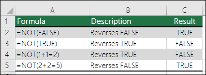
The NOT function reverses the value of its argument.

One common use for the NOT function is to expand the usefulness of other functions that perform logical tests. For example, the IF function performs a logical test and then returns one value if the test evaluates to TRUE and another value if the test evaluates to FALSE. By using the NOT function as the logical_test argument of the IF function, you can test many different conditions instead of just one.

Syntax

NOT(logical)

The NOT function syntax has the following arguments:

Logical Required. A value or expression that can be evaluated to TRUE or FALSE.

Remarks

If logical is FALSE, NOT returns TRUE; if logical is TRUE, NOT returns FALSE.

Examples

Here are some general examples of using NOT by itself, and in conjunction with IF, AND and OR.

Formula	Description
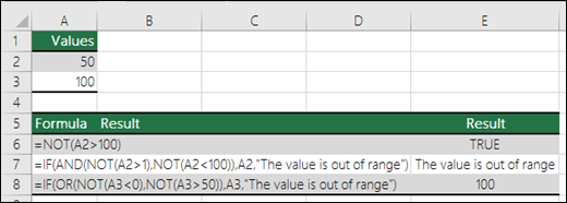
=NOT(A2>100)	A2 is NOT greater than 100
=IF(AND(NOT(A2>1),NOT(A2<100)),A2,»The value is out of range»)	50 is greater than 1 (TRUE), AND 50 is less than 100 (TRUE), so NOT reverses both arguments to FALSE. AND requires both arguments to be TRUE, so it returns the result if FALSE.
=IF(OR(NOT(A3<0),NOT(A3>50)),A3,»The value is out of range»)	100 is not less than 0 (FALSE), and 100 is greater than 50 (TRUE), so NOT reverses the arguments to TRUE/FALSE. OR only requires one argument to be TRUE, so it returns the result if TRUE.

Sales Commission Calculation

Here is a fairly common scenario where we need to calculate if sales people qualify for a bonus using NOT with IF and AND.

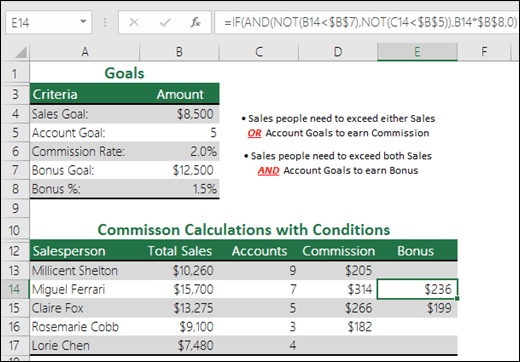
=IF(AND(NOT(B14<$B$7),NOT(C14<$B$5)),B14*$B$8,0)— IF Total Sales is NOT less than Sales Goal, AND Accounts are NOT less than the Account Goal, then multiply Total Sales by the Commission %, otherwise return 0.

Need more help?

You can always ask an expert in the Excel Tech Community or get support in the Answers community.

Check If Value In Range Using COUNTIF Function

Excel Find Value is in Range Example

How to check if a value is in Range with Wild Card Operators

Find if a Value is in a List Using MATCH Function

What is IFERROR Function in Excel?

Table of contents

Syntax

How to Use IFERROR Excel?

#1–“#N/A” Error

#2–“#DIV/0!” Error

#3–“#NAME?” Error

#4–“#NULL!” Error

#5–“#NUM!” Error

#6–“#REF!” Error

#7–“#VALUE!” Error

Frequently Asked Questions

Recommended Articles

NOT in Excel

NOT Formula in Excel

How to Use the NOT Function in Excel?

Example #1 – Excel NOT Function

Example #2 – Using NOT Function with ISBLANK

Example #3 – NOT Function along with “IF” and “OR” Function

Example #4 – VALUE! Error

Example #5 – NOT Function for an empty cell or blank or “0”

Example #6 – NOT Function for Decimals

Example #7 – NOT Function for Negative Number

Example #8 – When the value or Reference is Boolean Input in NOT Function

Recommended Articles

What’s on this page

1. Check if the cell contains any value in the list

1.1 Explaining formula in cell C3

Step 1 — Check if the cell contains any of the values in the list

Step 2 — Return TRUE if at least one value is 1

Step 3 — Return Yes or nothing

Regular formula

2. Display matches if the cell contains text from a list

2.1 Explaining formula in cell C3

Step 1 — Count cells containing text strings

Step 2 — Return the actual value

Step 3 — Concatenate values in array

3. Display matches if cell contains text from a list (Earlier Excel versions)

3.1 Explaining formula in cell C3

Step 1 — Identify matching values in cell

Step 2 — Calculate relative positions of matching values

Step 3 — Extract the k-th smallest number

Step 4 — Return value based on row number

Step 5 — Remove error values

4. Filter delimited values not in the list (Excel 365)

4.1 Explaining formula

Step 1 — Split values with a delimiting character

Step 2 — Remove leading and trailing spaces

Step 3 — Check if values are in list

Step 4 — Not

Step 5 — Filter

Step 6 — Join

Step 7 — Shorten the formula

Non-matching values

With INDEX

Что возвращает функция

Синтаксис

Аргументы функции

Дополнительная информация

Примеры использования функции NOT (НЕ) в Excel

Пример 1. Конвертируем значение TRUE (Истина) в FALSE (Ложь), и наоборот.

Пример 2. Используем функцию NOT (НЕ) с результатом формулы

Пример 3. Используем функцию NOT (НЕ) с числовыми значениями

Example

Examples

Need more help?

Related Topics

Need more help?

Want more options?