Not function for excel - Word и Excel - помощь в работе с программами

Excel for Microsoft 365 Excel for Microsoft 365 for Mac Excel for the web Excel 2021 Excel 2021 for Mac Excel 2019 Excel 2019 for Mac Excel 2016 Excel 2016 for Mac Excel 2013 Excel 2010 Excel 2007 Excel for Mac 2011 Excel Starter 2010 More…Less

Use the NOT function, one of the logical functions, when you want to make sure one value is not equal to another.

Example

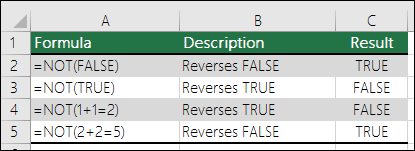
The NOT function reverses the value of its argument.

One common use for the NOT function is to expand the usefulness of other functions that perform logical tests. For example, the IF function performs a logical test and then returns one value if the test evaluates to TRUE and another value if the test evaluates to FALSE. By using the NOT function as the logical_test argument of the IF function, you can test many different conditions instead of just one.

Syntax

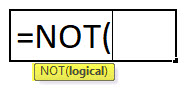
NOT(logical)

The NOT function syntax has the following arguments:

Logical Required. A value or expression that can be evaluated to TRUE or FALSE.

Remarks

If logical is FALSE, NOT returns TRUE; if logical is TRUE, NOT returns FALSE.

Examples

Here are some general examples of using NOT by itself, and in conjunction with IF, AND and OR.

Formula	Description
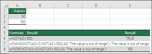
=NOT(A2>100)	A2 is NOT greater than 100
=IF(AND(NOT(A2>1),NOT(A2<100)),A2,»The value is out of range»)	50 is greater than 1 (TRUE), AND 50 is less than 100 (TRUE), so NOT reverses both arguments to FALSE. AND requires both arguments to be TRUE, so it returns the result if FALSE.
=IF(OR(NOT(A3<0),NOT(A3>50)),A3,»The value is out of range»)	100 is not less than 0 (FALSE), and 100 is greater than 50 (TRUE), so NOT reverses the arguments to TRUE/FALSE. OR only requires one argument to be TRUE, so it returns the result if TRUE.

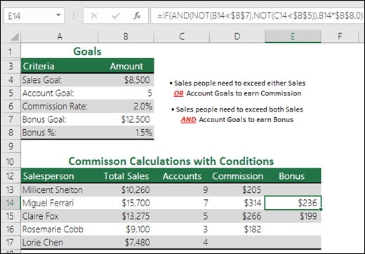
Sales Commission Calculation

Here is a fairly common scenario where we need to calculate if sales people qualify for a bonus using NOT with IF and AND.

=IF(AND(NOT(B14<$B$7),NOT(C14<$B$5)),B14*$B$8,0)— IF Total Sales is NOT less than Sales Goal, AND Accounts are NOT less than the Account Goal, then multiply Total Sales by the Commission %, otherwise return 0.

Need more help?

You can always ask an expert in the Excel Tech Community or get support in the Answers community.

Purpose

Reverse arguments or results

Usage notes

The NOT function returns the opposite of a given logical or Boolean value. Use the NOT function to reverse a Boolean value or the result of a logical expression.

When given FALSE, NOT returns TRUE.
When given TRUE, NOT returns FALSE.

Example #1 — not green or red

In the example shown, the formula in C5, copied down, is:

=NOT(OR(B5="green",B5="red"))

The literal translation of this formula is «NOT green or red». At each row, the formula returns TRUE if the color in column B is not green or red, and FALSE if the color is green or red.

Example #2 — Not blank

A common use case for the NOT function is to reverse the behavior of another function. For example, If cell A1 is blank (empty), the ISBLANK function will return TRUE:

=ISBLANK(A1)  // TRUE if A1 is empty

To reverse this behavior, wrap the NOT function around the ISBLANK function:

=NOT(ISBLANK(A1))  // TRUE if A1 is NOT empty

By adding NOT the output from ISBLANK is reversed. This formula will return TRUE when A1 is not empty and FALSE when A1 is empty. You might use this kind of test to only run a calculation if there is a value in A1:

=IF(NOT(ISBLANK(A1)),B1/A1,"")

Translation: if A1 is not blank, divide B1 by A1, otherwise return an empty string («»). This is an example of nesting one function inside another.

Источник

Функция NOT (НЕ) в Excel используется для изменения логического выражения TRUE (Истина) / FALSE (Ложь).

Содержание

Что возвращает функция
Синтаксис
Аргументы функции
Дополнительная информация
Примеры использования функции NOT (НЕ) в Excel
Пример 1. Конвертируем значение TRUE (Истина) в FALSE (Ложь), и наоборот.
Пример 2. Используем функцию NOT (НЕ) с результатом формулы
Пример 3. Используем функцию NOT (НЕ) с числовыми значениями

Что возвращает функция

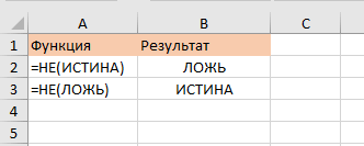
Логический аргумент, который является обратным логическому аргументу, используемому в функции NOT. Например, =NOT(TRUE) возвращает FALSE (Ложь) и =NOT(FALSE) возвращает TRUE(Истина).

Синтаксис

=NOT (logical) — английская версия

=НЕ(логическое_значение) — русская версия

Аргументы функции

logical (логическое значение) — значение или выражение, которое может быть логически оценено как TRUE (Истина) или FALSE (Ложь)

Дополнительная информация

С помощью функции NOT (НЕ) в Excel вы можете проверить выражение, которое принимает значение TRUE или FALSE. Например, =NOT(1 + 1 = 2) вернет FALSE.

Больше лайфхаков в нашем Telegram Подписаться

Примеры использования функции NOT (НЕ) в Excel

Пример 1. Конвертируем значение TRUE (Истина) в FALSE (Ложь), и наоборот.

Функция преобразует TRUE (Истина) в FALSE (Ложь) и FALSE (Ложь) в TRUE (Истина). Аргумент внутри функции также может быть результатом другой функции, результатом которой являются TRUE / FALSE.

Пример 2. Используем функцию NOT (НЕ) с результатом формулы

Если вы используете функцию с результатом какой-либо формулы (которая возвращает значения TRUE или FALSE), то она конвертирует результат TRUE в FALSE и наоборот. На примере выше, значение в ячейке А2 сравнивается с числом. По результату вычисления, при совпадении условий формулы, NOT (НЕ) выдаст FALSE, или отразит TRUE, если значение не совпадает с условиями.

Пример 3. Используем функцию NOT (НЕ) с числовыми значениями

В Excel, по умолчанию принято, что цифровое значение “0” (ноль) принимается за FALSE, а любое положительное значение — TRUE. Функция NOT (НЕ) при использовании с числами конвертирует “0” (ноль) в TRUE (Истина) и любое позитивное значение или отрицательное в FALSE (Ложь).

Источник

Перейти к содержанию

На чтение 1 мин Просмотров 226 Опубликовано 10.12.2021

Содержание

В каких случаях эта функция может пригодиться?
Что возвращает функция НЕ (NOT)?
Синтаксис
Используемые в формуле функции аргументы
Варианты использования функции НЕ (NOT)
Превращаем ИСТИНУ в ЛОЖЬ
Используем функцию вместе с вычислением
Пример использования НЕ (NOT) с числами

В каких случаях эта функция может пригодиться?

Идеально эта функция подойдет, когда необходимо поменять ИСТИНУ на ЛОЖЬ и наоборот.
Так же эту функцию можно использовать в условиях, когда нужно выбрать условия, отличные от того, что мы ищем.

Что возвращает функция НЕ (NOT)?

В результате выполнения этой функции вы получите логическое значение — Ложь или Истина

Синтаксис

=НЕ(любой_аргумент_имеющий_логическое_значение)

Используемые в формуле функции аргументы

любой_аргумент_имеющий_логическое_значение — например, 1+1=2 — это будет ИСТИНА.

Варианты использования функции НЕ (NOT)

Превращаем ИСТИНУ в ЛОЖЬ

Бывают ситуации, когда вам необходимо поменять значение на обратное. В такой ситуации, идеальным методом станет функция НЕ.

Используем функцию вместе с вычислением

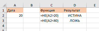
Также и в этом случае. Сначала происходит сравнение значения ячейки A2 с числом 20 и если A2>20 то вернется истина, а функция НЕ превратит его в ложь и так далее.

Пример использования НЕ (NOT) с числами

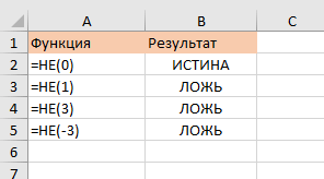
Мало кто знает, но в Excel у всех чисел есть логическое значение.

Например число 0 имеет значение ЛОЖЬ, а за истину принято считать 1

Источник

Date yes Add (Subtract) Days to a Date Concatenate Dates Convert Date to Number Convert Date to Text Month Name to Number Create Date Range from Dates Day Number of Year Month Name from Date First Day of Month Add (Subtract) Weeks to a Date If Functions with Dates Max Date Number of Days Between Dates Number of Days in a Month Number of Weeks Between Dates Number of Years Between Dates Split Date & Time into Separate Cells Countdown Remaining Days Insert Dates Random Date Generator Using Dynamic Ranges — Year to Date Values Add (Subtract) Years to a Date Date Formula Examples Extract Day from Date Get Day Name from Date Count Days Left in Month / Year Count Workdays Left in Month / Year Get Last Day of Month Last Business Day of Month / Year Number of Work / Business Days in Month Weekday Abbreviations Auto Populate Dates Number of Months Between Dates Quarter from a Date Years of Service Change Date Format Compare Dates Time yes Add (Subtract) Hours to Time Add (Subtract) Minutes to Time Add (Subtract) Seconds to Time Add Up time (Total Time) Time Differences Change Time Format Convert Minutes to Hours Convert Time to Decimal Convert Time to Hours Convert Time to Minutes Convert Time to Seconds Military Time Round Time to Nearest 15 Minutes Overtime Calculator Number of Hours Between Times Convert Seconds to Minutes, Hours, or Time Count Hours Worked Time Differences Time Format — Show Minutes Seconds Text yes Add Commas to Cells Get First Word from Text Capitalize First Letter Clean & Format Phone #s Remove Extra Trailing / Leading Spaces Add Spaces to Cell Assign Number Value to Text Combine Cells with Comma Combine First and Last Names Convert Text String to Date Convert Text to Number Extract Text From Cell Get Last Word Remove Unwated Characters Extract Text Before or After Character How to Split Text String by Space, Comma, & More Remove Special Characters Remove First Characters from Left Substitute Multiple Values Switch First & Last Names w/ Commas Remove Specific Text from a Cell Extract Text Between Characters (Ex. Parenthesis) Add Leading Zeros to a Number Remove Line Breaks from Text Remove all Numbers from Text Reverse Text Remove Non-Numeric Characters Remove Last Character(s) From Right Separate First and Last Names Separate Text & Numbers Round yes Round Formulas Round Price to Nearest Dollar or Cent Round to Nearest 10, 100, or 1000 Round to Nearest 5 or .5 Round Percentages Round to Significant Figures Count yes Count Blank and Non-blank Cells Count Cells Between Two Numbers Count Cells not Equal to Count if Cells are in Range Count Times Word Appears in Cell Count Words in Cell Count Specific Characters in Column Count Total Number of Characters in Column Count Cells that Equal one of two Results Count Cells that do not Contain Count Cells that Contain Specific Text Count Unique Values in Range Countif — Multiple Criteria Count Total Number of Cells in Range Count Cells with Any Text Count Total Cells in a Table Lookup yes Two Dimensional VLOOKUP VLOOKUP Simple Example Vlookup — Multiple Matches Case Sensitive Lookup Case Sensitive VLOOKUP Sum if — VLOOKUP Case Sensitive Lookup Case Sensitive VLOOKUP Find Duplicates w/ VLOOKUP or MATCH INDEX MATCH MATCH Lookup — Return Cell Address (Not Value) Lookup Last Value in Column or Row Reverse VLOOKUP (Right to Left) Risk Score Bucket with VLOOKUP Sum with a VLOOKUP Function VLOOKUP & INDIRECT VLOOKUP Concatenate VLOOKUP Contains (Partial Match) 17 Reasons Why Your XLOOKUP is Not Working Double (Nested) XLOOKUP — Dynamic Columns IFERROR (& IFNA) XLOOKUP Lookup Min / Max Value Nested VLOOKUP Top 11 Alternatives to VLOOKUP (Updated 2022!) VLOOKUP – Dynamic Column Reference VLOOKUP – Fix #N/A Error VLOOKUP – Multiple Sheets at Once VLOOKUP & HLOOKUP Combined VLOOKUP & MATCH Combined VLOOKUP Between Worksheets or Spreadsheets VLOOKUP Duplicate Values VLOOKUP Letter Grades VLOOKUP Return Multiple Columns VLOOKUP Returns 0? Return Blank Instead VLOOKUP w/o #N/A Error XLOOKUP Multiple Sheets at Once XLOOKUP Between Worksheets or Spreadsheets XLOOKUP by Date XLOOKUP Duplicate Values XLOOKUP Multiple Criteria XLOOKUP Return Multiple Columns XLOOKUP Returns 0? Return Blank Instead XLOOKUP Text XLOOKUP with IF XLOOKUP With If Statement Misc. yes Sort Multiple Columns Use Cell Value in Formula Percentage Change Between Numbers Percentage Breakdown Rank Values Add Spaces to Cell CAGR Formula Average Time Decimal Part of Number Integer Part of a Number Compare Items in a List Dealing with NA() Errors Get Worksheet Name Wildcard Characters Hyperlink to Current Folder Compound Interest Formula Percentage Increase Create Random Groups Sort with the Small and Large Functions Non-volatile Function Alternatives Decrease a Number by a Percentage Calculate Percent Variance Profit Margin Calculator Convert Column Number to Letter Get Full Address of Named Range Insert File Name Insert Path Latitute / Longitude Functions Replace Negative Values Reverse List Range Convert State Name to Abbreviation Create Dynamic Hyperlinks Custom Sort List with Formula Data Validation — Custom Formulas Dynamic Sheet Reference (INDIRECT) Reference Cell in Another Sheet or Workbook Get Cell Value by Address Get Worksheet Name Increment Cell Reference List Sheet Names List Skipped Numbers in Sequence Return Address of Max Value in Range Search by Keywords Select Every Other (or Every nth) Row Basics yes Cell Reference Basics — A1, R1C1, 3d, etc. Add Up (Sum) Entire Column or Row Into to Dynamic Array Formulas Conversions yes Convert Time Zones Convert Celsius to Fahrenheit Convert Pounds to Kilograms Convert Time to Unix Time Convert Feet to Meters Convert Centimeters to Inches Convert Kilometers to Miles Convert Inches to Feet Convert Date to Julian Format Convert Column Letter to Number Tests yes Test if a Range Contains any Text Test if any Cell in Range is Number Test if a Cell Contains a Specific Value Test if Cell Contains Any Number Test if Cell Contains Specific Number Test if Cell is Number or Text If yes Percentile If Subtotal If Sumproduct If Large If and Small If Median If Concatentate If Max If Rank If TEXTJOIN If Sum yes Sum if — Begins With / Ends With Sum if — Month or Year to Date Sum if — By Year Sum if — Blank / Non-Blank Sum if — Horizontal Sum Count / Sum If — Cell Color INDIRECT Sum Sum If — Across Multiple Sheets Sum If — By Month Sum If — Cells Not Equal To Sum If — Not Blank Sum if — Between Values Sum If — Week Number Sum Text Sum if — By Category or Group Sum if — Cell Contains Specific Text (Wildcards) Sum if — Date Rnage Sum if — Dates Equal Sum if — Day of Week Sum if — Greater Than Sum if — Less Than Average yes Average Non-Zero Values Average If — Not Blank Average — Ignore 0 Average — Ignore Errors Math yes Multiplication Table Cube Roots nth Roots Square Numbers Square Roots Calculations yes Calculate a Ratio Calculate Age KILLLLLLL Calculate Loan Payments GPA Formula Calculate VAT Tax How to Grade Formulas Find yes Find a Number in a Column / Workbook Find Most Frequent Numbers Find Smallest n Values Find nth Occurance of Character in Text Find and Extract Number from String Find Earliest or Latest Date Based on Criteria Find First Cell with Any Value Find Last Row Find Last Row with Data Find Missing Values Find Largest n Values Most Frequent Number Conditional Formatting yes Conditional Format — Dates & Times Conditional Format — Highlight Blank Cells New Functions XLOOKUP Replaces VLOOKUP, HLOOKUP, and INDEX / MATCH Logical yes AND Checks whether all conditions are met. TRUE/FALSE IF If condition is met, do something, if not, do something else. IFERROR If result is an error then do something else. NOT Changes TRUE to FALSE and FALSE to TRUE. OR Checks whether any conditions are met. TRUE/FALSE XOR Checks whether one and only one condition is met. TRUE/FALSE Lookup & Reference yes FALSE The logical value: FALSE. TRUE The logical value: TRUE. ADDRESS Returns a cell address as text. AREAS Returns the number of areas in a reference. CHOOSE Chooses a value from a list based on it’s position number. COLUMN Returns the column number of a cell reference. COLUMNS Returns the number of columns in an array. HLOOKUP Lookup a value in the first row and return a value. HYPERLINK Creates a clickable link. INDEX Returns a value based on it’s column and row numbers. INDIRECT Creates a cell reference from text. LOOKUP Looks up values either horizontally or vertically. MATCH Searches for a value in a list and returns its position. OFFSET Creates a reference offset from a starting point. ROW Returns the row number of a cell reference. ROWS Returns the number of rows in an array. TRANSPOSE Flips the oriention of a range of cells. VLOOKUP Lookup a value in the first column and return a value. Date & Time yes DATE Returns a date from year, month, and day. DATEDIF Number of days, months or years between two dates. DATEVALUE Converts a date stored as text into a valid date DAY Returns the day as a number (1-31). DAYS Returns the number of days between two dates. DAYS360 Returns days between 2 dates in a 360 day year. EDATE Returns a date, n months away from a start date. EOMONTH Returns the last day of the month, n months away date. HOUR Returns the hour as a number (0-23). MINUTE Returns the minute as a number (0-59). MONTH Returns the month as a number (1-12). NETWORKDAYS Number of working days between 2 dates. NETWORKDAYS.INTL Working days between 2 dates, custom weekends. NOW Returns the current date and time. SECOND Returns the second as a number (0-59) TIME Returns the time from a hour, minute, and second. TIMEVALUE Converts a time stored as text into a valid time. TODAY Returns the current date. WEEKDAY Returns the day of the week as a number (1-7). WEEKNUM Returns the week number in a year (1-52). WORKDAY The date n working days from a date. WORKDAY.INTL The date n working days from a date, custom weekends. YEAR Returns the year. YEARFRAC Returns the fraction of a year between 2 dates. Engineering yes CONVERT Convert number from one unit to another. Financial yes FV Calculates the future value. PV Calculates the present value. NPER Calculates the total number of payment periods. PMT Calculates the payment amount. RATE Calculates the interest Rate. NPV Calculates the net present value. IRR The internal rate of return for a set of periodic CFs. XIRR The internal rate of return for a set of non-periodic CFs. PRICE Calculates the price of a bond. YIELD Calculates the bond yield. INTRATE The interest rate of a fully invested security. Information yes CELL Returns information about a cell. ERROR.TYPE Returns a value representing the cell error. ISBLANK Test if cell is blank. TRUE/FALSE ISERR Test if cell value is an error, ignores #N/A. TRUE/FALSE ISERROR Test if cell value is an error. TRUE/FALSE ISEVEN Test if cell value is even. TRUE/FALSE ISFORMULA Test if cell is a formula. TRUE/FALSE ISLOGICAL Test if cell is logical (TRUE or FALSE). TRUE/FALSE ISNA Test if cell value is #N/A. TRUE/FALSE ISNONTEXT Test if cell is not text (blank cells are not text). TRUE/FALSE ISNUMBER Test if cell is a number. TRUE/FALSE ISODD Test if cell value is odd. TRUE/FALSE ISREF Test if cell value is a reference. TRUE/FALSE ISTEXT Test if cell is text. TRUE/FALSE N Converts a value to a number. NA Returns the error: #N/A. TYPE Returns the type of value in a cell. Math yes ABS Calculates the absolute value of a number. AGGREGATE Define and perform calculations for a database or a list. CEILING Rounds a number up, to the nearest specified multiple. COS Returns the cosine of an angle. DEGREES Converts radians to degrees. DSUM Sums database records that meet certain criteria. EVEN Rounds to the nearest even integer. EXP Calculates the exponential value for a given number. FACT Returns the factorial. FLOOR Rounds a number down, to the nearest specified multiple. GCD Returns the greatest common divisor. INT Rounds a number down to the nearest integer. LCM Returns the least common multiple. LN Returns the natural logarithm of a number. LOG Returns the logarithm of a number to a specified base. LOG10 Returns the base-10 logarithm of a number. MOD Returns the remainder after dividing. MROUND Rounds a number to a specified multiple. ODD Rounds to the nearest odd integer. PI The value of PI. POWER Calculates a number raised to a power. PRODUCT Multiplies an array of numbers. QUOTIENT Returns the integer result of division. RADIANS Converts an angle into radians. RAND Calculates a random number between 0 and 1. RANDBETWEEN Calculates a random number between two numbers. ROUND Rounds a number to a specified number of digits. ROUNDDOWN Rounds a number down (towards zero). ROUNDUP Rounds a number up (away from zero). SIGN Returns the sign of a number. SIN Returns the sine of an angle. SQRT Calculates the square root of a number. SUBTOTAL Returns a summary statistic for a series of data. SUM Adds numbers together. SUMIF Sums numbers that meet a criteria. SUMIFS Sums numbers that meet multiple criteria. SUMPRODUCT Multiplies arrays of numbers and sums the resultant array. TAN Returns the tangent of an angle. TRUNC Truncates a number to a specific number of digits. Stats yes AVERAGE Averages numbers. AVERAGEA Averages numbers. Includes text & FALSE =0, TRUE =1. AVERAGEIF Averages numbers that meet a criteria. AVERAGEIFS Averages numbers that meet multiple criteria. CORREL Calculates the correlation of two series. COUNT Counts cells that contain a number. COUNTA Count cells that are non-blank. COUNTBLANK Counts cells that are blank. COUNTIF Counts cells that meet a criteria. COUNTIFS Counts cells that meet multiple criteria. FORECAST Predict future y-values from linear trend line. FREQUENCY Counts values that fall within specified ranges. GROWTH Calculates Y values based on exponential growth. INTERCEPT Calculates the Y intercept for a best-fit line. LARGE Returns the kth largest value. LINEST Returns statistics about a trendline. MAX Returns the largest number. MEDIAN Returns the median number. MIN Returns the smallest number. MODE Returns the most common number. PERCENTILE Returns the kth percentile. PERCENTILE.INC Returns the kth percentile. Where k is inclusive. PERCENTILE.EXC Returns the kth percentile. Where k is exclusive. QUARTILE Returns the specified quartile value. QUARTILE.INC Returns the specified quartile value. Inclusive. QUARTILE.EXC Returns the specified quartile value. Exclusive. RANK Rank of a number within a series. RANK.AVG Rank of a number within a series. Averages. RANK.EQ Rank of a number within a series. Top Rank. SLOPE Calculates the slope from linear regression. SMALL Returns the kth smallest value. STDEV Calculates the standard deviation. STDEV.P Calculates the SD of an entire population. STDEV.S Calculates the SD of a sample. STDEVP Calculates the SD of an entire population TREND Calculates Y values based on a trendline. Text yes CHAR Returns a character specified by a code. CLEAN Removes all non-printable characters. CODE Returns the numeric code for a character. CONCATENATE Combines text together. DOLLAR Converts a number to text in currency format. EXACT Test if cells are exactly equal. Case-sensitive. TRUE/FALSE FIND Locates position of text within a cell.Case-sensitive. LEFT Truncates text a number of characters from the left. LEN Counts number of characters in text. LOWER Converts text to lower case. MID Extracts text from the middle of a cell. PROPER Converts text to proper case. REPLACE Replaces text based on it’s location. REPT Repeats text a number of times. RIGHT Truncates text a number of characters from the right. SEARCH Locates position of text within a cell.Not Case-sensitive. SUBSTITUTE Finds and replaces text. Case-sensitive. TEXT Converts a value into text with a specific number format. TRIM Removes all extra spaces from text. UPPER Converts text to upper case. VALUE Converts a number stored as text into a number.

Источник

The NOT Excel function is a logical function in Excel called the negation function. It negates the value returned through a function or a value from another logical function. This built-in function in Excel takes a single argument: the logic, which can be a formula or a logical value.

For example, suppose we inserted the Excel NOT function in the dataset and conducted the logical test. As a result, it may return the opposite of a given logical or Boolean value. Suppose one value is TRUE, NOT function returns as FALSE. And when the given value is FALSE, NOT function may return TRUE. The NOT function can reverse a logical value.

NOT Function in Excel
- Syntax
  - Compulsory Parameter:
- Examples
  - Example #1
  - Example #2
  - Example #3
  - Example #4
- Recommended Articles

Syntax

Compulsory Parameter:

Logical: The numeric value 0 is considered “False,” and the rest of the values are considered “True.” Logical is an expression that either calculates the TRUE or FALSE if it returns TRUE if the expression is FALSE and returns FALSE if the expression is TRUE.

Examples

You can download this NOT Function Excel Template here – NOT Function Excel Template

Example #1

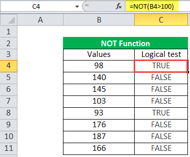
We must check which value is greater than 100; then, we can use the NOT function in the Logical testA logical test in Excel results in an analytical output, either true or false. The equals to operator, “=,” is the most commonly used logical test.read more column. It will return the reverse return if the value is greater than 100, then it will return FALSE, and if the value is less than or equal to 100, it will return the TRUE as output.

Example #2

Let us consider another example wherein we must exclude the color combination red and blue from the toy data set. Then, we can use the NOT function to filter out this combination. But, again, the output will be TRUE because the color is red here.

Example #3

Let us take the employee data wherein we must find the bonus amount for employees who did the extra task and no bonus for those who did not perform the additional task, and employees get ₹100 for each extra task.

The output will be = ₹7500 as it will first check for a blank entry in a cell. If not empty, it will multiply the extra task and 100 to calculate the bonus unlocked by the employee.

Example #4

Suppose we have to check colors, such as for the example below, we have to filter out the toy name with the color blue or red from the given data set.

First, this will check the condition if the color column contains any toy with blue or red if the condition is TRUE, then it will return blank as output; if not TRUE, it will return x as output.

Syntax

The unfussy syntax of the NOT function is as follows:

=NOT(logical)

Arguments:

logical – The value or condition to be tested.

Important Characteristics of NOT Function in Excel

NOT function returns either «TRUE» or «FALSE» and can evaluate up to 255 conditions.
If an argument is the number 0, the result will be «TRUE». Excel processes 0 as FALSE. The NOT function changes FALSE to TRUE.
If no logical values are found in the formula, the function returns a #VALUE! error.
If the formula has any typos or misspelling, the function returns a #NAME?
The arguments can be numbers, cell references, defined names, formulas, functions, or text.

Examples of NOT Function

The talk is better when practically put to the test. So let’s see some examples to understand why the NOT function does the opposite of what it’s told.

Example 1 – Super Duper Basic NOT Function

Riddle time.

Question – What is not TRUE?
Answer: FALSE

Question – What is not FALSE?
Answer: TRUE

See how easy that was? That wasn’t even in Excel language. Working with Boolean parameters, bringing out this function’s ability could not get simpler than this:

=NOT(TRUE) //returns "FALSE" =NOT(FALSE) //returns "TRUE"

We’re making the NOT function’s life too easy. We can make it work harder.

Example 2 – Plain Vanilla Version of NOT Function

Let’s say Gina loves granola. We have granola bars enlisted with allergens that they contain since Gina has a severe peanut allergy.

Our objective here is to pick out the bars that contain peanuts so Gina can steer clear of them. That’s achievable with this formula:

=NOT(B2 = "Peanut")

What this formula is doing is looking up column B for the word «Peanut». Since the command is for the cell to not contain «Peanut», if the word «Peanut» is found, the result would be «FALSE». If it is not found, the result will be «TRUE».

Cell «C2» asks cell «B2» ‘NOT Peanut?’. «B2» is blank, it’s TRUE, «B2» is ‘NOT Peanut’.
Cell «C4» asks cell «B4» ‘NOT Peanut?’. «B4» is «Peanut», it’s FALSE.

Gina has to keep away from the «FALSE» results. Luckily, she has a lot of peanut-free options.

Example 3 – Use of NOT Function with IF Function

The role of an IF function is to return a value based on a stated condition. Bringing forward the example from above, we take a look at how the 2 functions go together.

The plus point here of using the NOT function within the IF function is that we can get:

«Peanut Free!» instead of «TRUE» and
«Peanuts Present!» instead of «FALSE»

as a result.

We use the following formula:

=IF(NOT(B2 = "Peanut"), "Peanut Free!", "Peanuts Present!")

Firstly, the NOT function starts its work, looks up the «B2» cell to check whether it contains «Peanut». NOT function finds «B2» cell blank, which implies «B2» is «NOT» equal to «Peanut». And thus, the result of the NOT function is «TRUE».

The result is passed onto the IF function where the corresponding value for TRUE is «Peanut Free!». Hence the IF function returns «Peanut Free!» as a result.

Example 4 – NOT «X» OR «Y»

The OR function can be used to evaluate an array of values and determine whether the condition specified is met in at least one value or not. Let’s carry forward the example above.

It turns out Gina isn’t as lucky as we thought; she is also allergic to soy! Which means her favorite granola bars need to be peanut and soy-free. Let’s help her.

We need to find granola bars that do not contain peanuts or soy. To find these two allergens, the formula we’ve applied is:

=NOT(OR(B2 = "Peanut", B2 = "Soy"))

The OR function has been asked to check cells from B2 to B17 and see whether they contain

«Peanut» or
«Soy».

The OR function finds «B2» contains «Soy». Since one argument of the function is fulfilled, the result is «TRUE». This result is passed onto the NOT function.

The NOT function flips «TRUE» to «FALSE».

The core purpose of having the NOT function here anyway is to find out whether «B2» is NOT «Peanut» OR «Soy». So as the greater picture, the result is also «FALSE» and that is the result returned in C2.

IF NOT «x» OR «y»

To attain the same customized result seen in Example 3, we can easily incorporate the IF function by this formula:

=IF(NOT(OR(B2 = "Peanut", B2 = "Soy")),"Safe!","Unsafe!")

The results are in column C. Adding the IF function has customized the results into:

«Safe!» instead of «TRUE» and
«Unsafe!» instead of «FALSE».

That would be it. NOT the last you hear from us. Since we talked so much about granola bars, you know what else you can do on Excel?

You can make a pie chart of your favorite bars.

And a bar graph of your favorite pies.

We’ll be back with more… functions, not jokes.

Источник

NOT in Excel

NOT function is an inbuilt function that is categorized under the Logical Function; the logical function operates under a logical test. It is also called Boolean logic or function. Boolean functions are most commonly used along with or in conjunction with other functions, specifically along with conditional test functions (“IF’’ FUNCTION), to create formulas that can evaluate multiple parameters or criteria and produce desired results depending on that criteria. It is used as an individual function or part of the formula and other excel functions in a cell. E.G. with AND, IF & OR function. It returns the opposite value of a given logical value in the formula, NOT function is used to reverse a logical value. If the argument is FALSE, then TRUE is returned and vice versa.

Note: Use NOT function when you want to make sure a value is not equal to one Specific or particular value

It’s a worksheet function; it is also used as part of the formula in a cell along with other excel function

If given with the value TRUE, the Not function returns FALSE
If given with the value FALSE, the Not function returns TRUE

NOT Formula in Excel

Below is the NOT Formula in excel:

=NOT (logical) logical – A value that can be evaluated to TRUE or FALSE

The only parameter in the NOT function is a logical value.

The logical test or argument can be either entered directly, or it can be entered as a reference to a cell that contains a logical value, and it always returns the Boolean value (“TRUE” OR “FALSE”) only.

How to Use the NOT Function in Excel?

NOT Function in Excel is very simple and easy to use. Let us now see how to use the NOT function in excel with the help of some examples.

You can download this NOT function Excel Template here – NOT function Excel Template

Example #1 – Excel NOT Function

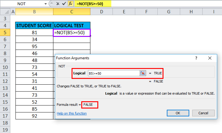
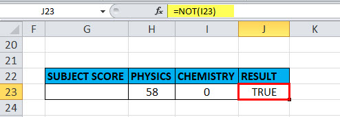
Here a logical test is performed on the given set of values (Student score) by using the NOT function. Here, we will check which value is greater than or equal to 50.

In the table, we have 2 columns, the first column contains student score & the second column is the logical test column, where the NOT function is performed.

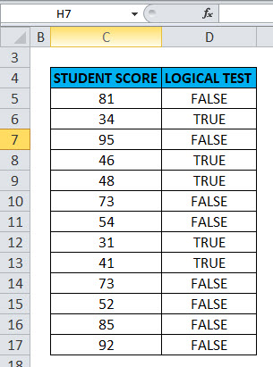
Result: It will return the reverse value if the value is greater than or equal to 50, then it will return FALSE and if the lesser than or equal to 50, it will return TRUE as output.

The result will be as given below:

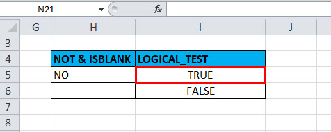
Example #2 – Using NOT Function with ISBLANK

the logical test is performed on the H5 & H6 Cells by using the NOT Function along with ISBLANK function; here will check if cells H5 & H6 is blank OR not using NOT function along with ISBLANK in excel

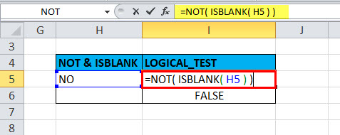
OUTPUT will be TRUE.

Example #3 – NOT Function along with “IF” and “OR” Function

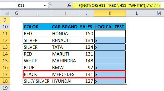
Here the color check is performed for the cars in the below-mentioned table by using NOT Function along with “if” and “or” function

Here we have to sort out color “WHITE” or “RED” from the given set of data

=IF(NOT(OR(H11=”RED”,H11=”WHITE”)),”x”,””) formula is used

This logical condition is applied on a Color column containing any car with color “RED” or “WHITE”,

if the condition is true, then it will return blank as output,

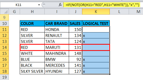
if not true, then it will return x as output

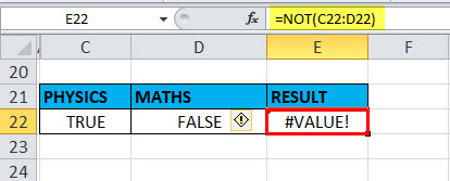
Example #4 – VALUE! Error

It Occurs when the supplied argument is not a logical or numeric value.

Suppose, if we give a range in the logical argument

Selected the range C22:D22 in the logical argument, i.e. =NOT (C22:D22)

a function returns a #VALUE error because the NOT function does not allow any range and can take only a logical test or argument or one condition.

Example #5 – NOT Function for an empty cell or blank or “0”

An empty cell or blank or “0” are treated as false, therefore “NOT” function returns TRUE

Here in the cell “I23”, the stored value is “0” suppose if I apply the “NOT” function with logical argument or value as “0” or “I23”, Output will be TRUE.

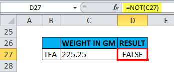
Example #6 – NOT Function for Decimals

When the value is decimal in a cell

Suppose if we take the argument as decimals, i.e. suppose if I apply the “NOT” function with logical argument or value as “225.25” or “c27”, Output will be FALSE.

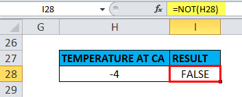
Example #7 – NOT Function for Negative Number

When the value is a negative number in a cell

Suppose if we take the argument as a negative number, i.e. suppose if I apply the “NOT” function with logical argument or value as “-4” or “H27”, Output will be FALSE.

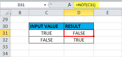
Example #8 – When the value or Reference is Boolean Input in NOT Function

When the value or reference is Boolean input (“TRUE” OR “FALSE”) in a cell.

Here in the cell “C31”, the stored value is “TRUE” suppose if I apply the “NOT” function with logical argument or value as “C31” or “TRUE”, Output will be FALSE. It will be vice versa if the logical argument is “FALSE”, i.e. the NOT function returns the “TRUE” value as output.

Синтаксис функции

НЕ(логическое_значение)

логическое_значение

— любое значение или выражение, принимающее значения ИСТИНА или ЛОЖЬ.

=НЕ(A1>100)

Т.е. если в одной ячейке

A1

содержится значение больше 100, то формула вернет

ЛОЖЬ,

а если <=100, то —

ИСТИНА

.

Другими словами, формула

=НЕ(ЛОЖЬ)

вернет ИСТИНА, а формула

=НЕ(ИСТИНА)

вернет ЛОЖЬ.

Совместное использование с другими функциями

Сама по себе функция

НЕ()

имеет ограниченное использование, т.к. она может вернуть только значения ИСТИНА или ЛОЖЬ.

Предположим, что проверяется 2 значения на превышение числа 100:

=И(A1>100;A2>100)

Пусть необходимо вернуть значение ИСТИНА, когда оба значения

НЕ

превышают 100. Этого можно добиться изменив формулу на

=И(A1<=100;A2<=100)

или просто записав

=НЕ(И(A1>100;A2>100))

Другой пример, ответим на вопрос «Содержит ли ячейка

А1

какое-нибудь значение». Для этого можно записать формулу

=НЕ(ЕПУСТО(A1))

. Формула вернет ИСТИНА, если ячейка

А1

содержит значение.

Источник

Excel NOT Function (Example + Video)

When to use Excel NOT Function

It can be used when you want to reverse the value of a logical argument (TRUE/FALSE).

What it Returns

It returns a logical argument which is the reverse of the logical argument used within the NOT function. For example, =NOT(TRUE) returns FALSE and =NOT(FALSE) returns TRUE.

Syntax

=NOT(logical)

Input Arguments

logical – A value or expression that can be evaluated to TRUE or FALSE.

Additional Notes:

You can check expression with NOT function that evaluates to TRUE or FALSE.
- For example, =NOT(1+1=2) would return FALSE.

Examples – Using Excel NOT Function

Here are three example of using the Excel NOT Function:

#1 Converting TRUE to FALSE / FALSE to TRUE

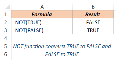
It converts TRUE to FALSE and FALSE to TRUE. The argument within the function can also be a result of some other function(s) that results in TRUE/FALSE.

#2 Using with Formula Result

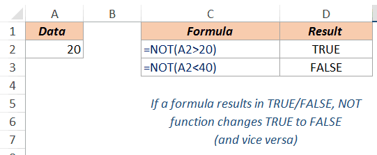
If used with a formula result (that returns TRUE/FALSE), it converts TRUE to FALSE and FALSE to TRUE. In the above example, the value is A2 is compared with a number (that returns TRUE if the condition is met, else FALSE), and NOT function is used on the result of the comparison.

#3 Using with Numbers

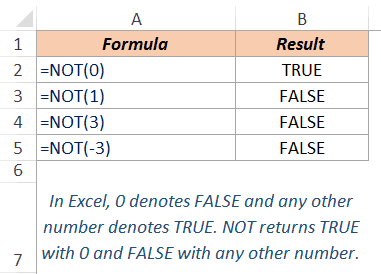
In Excel, 0 denotes FALSE and any other number denotes TRUE. Excel NOT function converts 0 (which is FALSE) to TRUE and any other number to FALSE.

Excel NOT Function – Video Tutorial

Related Excel Functions:

Excel AND Function.
Excel OR Function.
Excel IF Function.
Excel IFS Function.
Excel IFERROR Function.
Excel FALSE Function.
Excel TRUE Function.

Источник

Example

Examples

Need more help?

Related Topics

Need more help?

Want more options?

Purpose

Usage notes

Example #1 — not green or red

Example #2 — Not blank

Что возвращает функция

Синтаксис

Аргументы функции

Дополнительная информация

Примеры использования функции NOT (НЕ) в Excel

Пример 1. Конвертируем значение TRUE (Истина) в FALSE (Ложь), и наоборот.

Пример 2. Используем функцию NOT (НЕ) с результатом формулы

Пример 3. Используем функцию NOT (НЕ) с числовыми значениями

В каких случаях эта функция может пригодиться?

Что возвращает функция НЕ (NOT)?

Синтаксис

Используемые в формуле функции аргументы

Варианты использования функции НЕ (NOT)

Превращаем ИСТИНУ в ЛОЖЬ

Используем функцию вместе с вычислением

Пример использования НЕ (NOT) с числами

Table of contents

Syntax

Compulsory Parameter:

Examples

Example #1

Example #2

Example #3

Example #4

Recommended Articles

Syntax

Important Characteristics of NOT Function in Excel

Examples of NOT Function

Example 1 – Super Duper Basic NOT Function

Example 2 – Plain Vanilla Version of NOT Function

Example 3 – Use of NOT Function with IF Function

Example 4 – NOT «X» OR «Y»

NOT in Excel

NOT Formula in Excel

How to Use the NOT Function in Excel?

Example #1 – Excel NOT Function

Example #2 – Using NOT Function with ISBLANK

Example #3 – NOT Function along with “IF” and “OR” Function

Example #4 – VALUE! Error

Example #5 – NOT Function for an empty cell or blank or “0”

Example #6 – NOT Function for Decimals

Example #7 – NOT Function for Negative Number

Example #8 – When the value or Reference is Boolean Input in NOT Function

Recommended Articles

Синтаксис функции

Совместное использование с другими функциями

Excel NOT Function (Example + Video)

When to use Excel NOT Function

What it Returns

Syntax

Input Arguments

Additional Notes:

Examples – Using Excel NOT Function

#1 Converting TRUE to FALSE / FALSE to TRUE

#2 Using with Formula Result

#3 Using with Numbers

Excel NOT Function – Video Tutorial