No negatives in excel

Negative Numbers in Excel

Excel Negative Numbers

Microsoft Excel uses positive and negative numbers in performing mathematical calculations. In Excel, negative numbers are displayed with minus symbols by default. These are the numbers that are lower than 0 in value. Excel makes it easy to recognize the negative numbers by facilitating various best practices.

It needs to recognize the negative numbers while performing the calculations. In some scenarios, such as determining variance, it is necessary to convert the negative numbers to positive numbers or represent them in an appropriate format to use the negative values appropriately. It is required to represent them by applying a specific conditional format Conditional Format Conditional formatting is a technique in Excel that allows us to format cells in a worksheet based on certain conditions. It can be found in the styles section of the Home tab. read more based on the requirement.

The present article aims to identify ways to manage the negative numbers in Excel.

Table of contents

Explanation of Negative Numbers in Excel

Handling the negative numbers is very easy in Excel. Excel can manage both positive and negative numbers effectively. But, negative numbers can generate some confusion for the users sometimes. There is a chance for the occurrence of issues while handling negative numbers when the inappropriate format is chosen for them. It displays the errors when a user tries to perform calculations on the negatives.

Entering the negative numbers with a minus sign is very easy but analyzing them is tough when a mixture of positive and negative values is presented. To avoid this problem, it needs to change the format of the Excel cells that contain negative values to get accurate results.

You are free to use this image on your website, templates, etc., Please provide us with an attribution link How to Provide Attribution? Article Link to be Hyperlinked
For eg:
Source: Negative Numbers in Excel (wallstreetmojo.com)

How to Show Negative Numbers in Excel?

Negative numbers have a lot of significance in handling the various applications in Excel. Therefore, applying the set of formats is important in multiple areas.

Top 3 Ways to Show/Highlight Negative Numbers in Excel

This section will describe the various ways to show/highlight negative numbers in Excel.

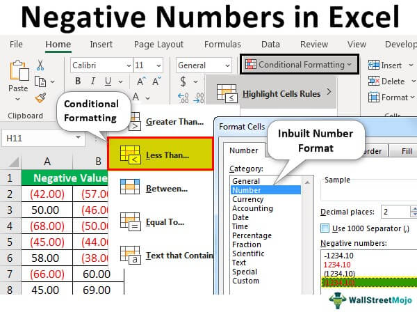
Example#1 – With Conditional Formatting

Representing negative numbers with conditional formatting

This example illustrates the Excel conditional formatting to highlight the negative numbers in various steps. For this example, we need to use numbers that are lower than 0.

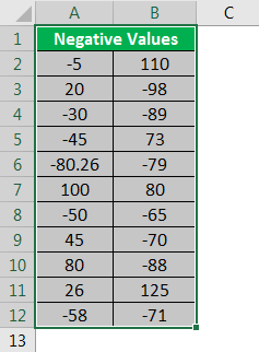
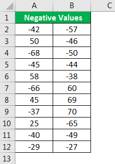
The following data is considered to illustrate this example.

Step 1: We must first select the entire range of data as shown in the figure.

Then, go to the “Home” tab and select conditional formatting. Next, select the “Highlight Cells Rules” and “Less Than” under the options presented.

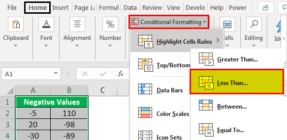
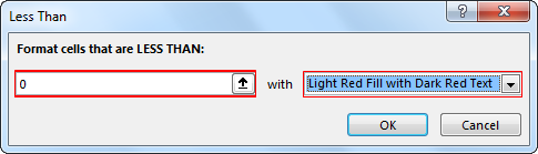
It opens the “Less Than” dialog box, as shown in the figure.

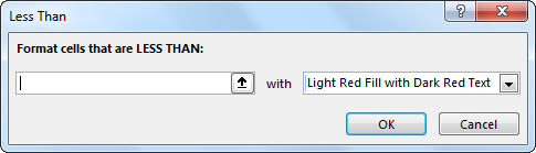
Step 2: Enter the value in the empty box under “Format cells that are LESS THAN” and click on the dropdown right to “with’ to apply the desired formatting to the numbers. Ensure that “Light Red Fill with Dark Red Text” is highlighted. Then click on “OK.”

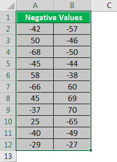
The output is shown as,

The above figure identifies that the cells with values less than 0 are highlighted with a red fill and red color to text. This type of conditional formatting is also applied with greater than, between, equal to, and duplicate values with negative values.

Example#2 – With Inbuilt Number Formatting

Representing negative numbers with inbuilt number formatting

This example is to illustrate the Excel inbuilt number formatting to highlight the negative numbers in red color. For this example, we need to use numbers that are lower than 0. The following are the steps required

The following data is considered to illustrate this example.

Step 1: Select the data that you want to apply the inbuilt custom formatting with a red color.

Step 2:

• Go to the “Home” tab.
• Click on “Number Format.”
• Click on the small tilted icon on the right side corner.

It helps in opening the “Format Cells” dialog box.

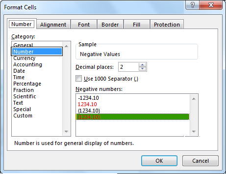
Step 3: In the “Format Cells” dialog box, ensure that the “Number” tab is highlighted in the “Format Cells” dialog box. Go to “Number” under the “Number” tab. Select the red text option with brackets for negative numbers on the right side of the options. And click on “OK.”

Step 4: The formatted Excel negative numbers will look as follows,

Two decimal points are automatically added to numbers when the formatting is applied.

Example#3 – With Custom Number Formatting

Representing negative numbers with custom number formatting

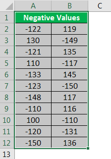
The following data is considered to illustrate this example.

Step 1: We must select the data that we want to apply the inbuilt custom formatting with a red color.

Step 2: Go to the “Home” tab.

• Click on “Number format’.”
• Click on the small tilted icon on the right side.

It helps in opening the “Format Cells” dialog box.

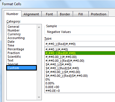
Step 3: The dialog box ensures that the “Number” tab is highlighted in the “Format Cells.” Go to the “Custom” option under the “Number” tab. Select the appropriate format, as shown in the figure. Click on “OK” to apply the formatting.

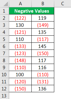
Step 4: The negative numbers will look as follows in Excel.

Things to Remember

• Conditional formatting is volatile. Whenever values change in the Excel sheet, it reassesses the condition and changes the formatting of the dataset. Therefore, it will become a problem for large datasets.
• We can apply any color to the background and text in Excel cells to highlight the negative numbers.

Recommended Articles

This article is a guide to Negative Numbers in Excel. We discuss how to show/highlight the negative number in Excel with the help of examples. You can learn more about Excel from the following articles: –

Источник

Negative numbers aren’t showing with parentheses in Excel

If you’re using Excel and negative numbers aren’t displaying with parentheses, you can change the way negative numbers are displayed. But if that doesn’t work, or if the parentheses option ($1,234.10) isn’t available, it’s likely because an operating system setting isn’t set properly. If you’re using a Mac, make sure you use the App Store and update to the latest version of macOS. If you’re using Windows, use one of the following solutions to change the negative number format. Keep in mind that changing the setting will affect all programs on your computer, not just Excel.

Change negative number formats in Windows

From the Start menu, search for Control Panel, and open Control Panel.

Under Clock, Language, and Region, click Change date, time, or number formats.

Note: If you don’t see Clock, Language, and Region, click Category in the View by menu at the top of the page.

On the Formats tab, click Additional settings at the bottom.

On the Numbers tab, for Negative number format, choose (1.1)

On the Currency tab, for Negative currency format, choose ($1.1)

Click OK, and then click OK again.

Click Start > Control Panel.

Under Clock, Language, and Region, click Change keyboards or other input methods.

Note: If you don’t see Clock, Language, and Region, click Category in the View by menu at the top.

On the Formats tab, click Additional settings at the bottom.

On the Numbers tab, for Negative number format, choose (1.1)

On the Currency tab, for Negative currency format, choose ($1.1)

Click OK, and then click OK again.

Click Start > Control Panel.

Under Clock, Language, and Region, click Change keyboards or other input methods.

Note: In Classic View, double-click Regional and Language Options, and then click the Formats tab.

On the Formats tab, click Additional settings at the bottom.

On the Numbers tab, for Negative number format, choose (1.1)

On the Currency tab, for Negative currency format, choose ($1.1)

Click OK, and then click OK again.

Click Start > Settings > Control Panel.

Click Date, Time, Language, and Regional Options, and then click Regional and Language Options.

Note: In Classic View, double-click Regional and Language Options, and then click the Formats tab.

On the Formats tab, click Additional settings at the bottom.

On the Numbers tab, for Negative number format, choose (1.1)

On the Currency tab, for Negative currency format, choose ($1.1)

Источник

Displaying Negative Numbers in Parentheses – Excel

This article will show you how to display negative numbers in parenthesis.

Negative numbers in Excel

In Excel, the basic way to format negative numbers is to use the Accounting number format.

This option will display your negative number in red.

But for some reports, negative numbers must be displayed with parenthesis. Let’s see how to do that.

Customize your number format

To display your negative numbers with parentheses, we must create our own number format.

Open the dialog box «Format Cells» using the shortcut Ctrl + 1 or by clicking on the last option of the Number Format dropdown list.

Or by clicking on this icon in the ribbon

Code to customize numbers in Excel

Excel can return 4 different display formats for a number. There are parameters for:

• 1st position: Format for Positive value
• 2nd position: Format for Negative value
• 3rd position: Format for Zero
• 4th position: Format for Text

The order of the parameters are:

Positive value;Negative value;Zero;Text

You also need to specify how the number will be returned.

• Use 0 to display number or 0 if empty
• Use # to display number or nothing

For instance, if you have the number 123

• The code #### will return 123
• With the code 0000 the display will be 0123
• And with the code ###0.00 the display will be 123.00

Code to return negative number in parenthesis

So with this information, we can easily create a format for negative numbers between parentheses.

• For the positive number: ###0.00
• For the negative number in parentheses: (###0.00)

The code you need to enter in the «Type» field is:

So you write this code in the Custom field of the Format Number

The display of negative numbers is now 😀😎😍

And if you also want to add the color red for those numbers, you just add the color setting in to code between bracket.

Start Excel with your custom parameters

You can save your customs format number in a template and load then when you open a new workbook. The method is explain in this article.

Источник

Microsoft Excel uses positive and negative numbers in performing mathematical calculations. In Excel, negative numbers are displayed with minus symbols by default. These are the numbers that are lower than 0 in value. Excel makes it easy to recognize the negative numbers by facilitating various best practices.

It needs to recognize the negative numbers while performing the calculations. In some scenarios, such as determining variance, it is necessary to convert the negative numbers to positive numbers or represent them in an appropriate format to use the negative values appropriately. It is required to represent them by applying a specific conditional formatConditional formatting is a technique in Excel that allows us to format cells in a worksheet based on certain conditions. It can be found in the styles section of the Home tab.read more based on the requirement.

The present article aims to identify ways to manage the negative numbers in Excel.

Explanation of Negative Numbers in Excel

Handling the negative numbers is very easy in Excel. Excel can manage both positive and negative numbers effectively. But, negative numbers can generate some confusion for the users sometimes. There is a chance for the occurrence of issues while handling negative numbers when the inappropriate format is chosen for them. It displays the errors when a user tries to perform calculations on the negatives.

Entering the negative numbers with a minus sign is very easy but analyzing them is tough when a mixture of positive and negative values is presented. To avoid this problem, it needs to change the format of the Excel cells that contain negative values to get accurate results.

You are free to use this image on your website, templates, etc, Please provide us with an attribution linkArticle Link to be Hyperlinked
For eg:
Source: Negative Numbers in Excel (wallstreetmojo.com)

How to Show Negative Numbers in Excel?

Negative numbers have a lot of significance in handling the various applications in Excel. Therefore, applying the set of formats is important in multiple areas.

• Financial analysts use a best practice in financial modelingFinancial modeling refers to the use of excel-based models to reflect a company’s projected financial performance. Such models represent the financial situation by taking into account risks and future assumptions, which are critical for making significant decisions in the future, such as raising capital or valuing a business, and interpreting their impact.read more representing the negative values in red.
• Negative numbers are squared in the determination of variance in data analysis to remove the problem presented with standard deviation.
• When the variance value is negative, it is multiplied by -1 to make it positive.
• In VBA, negative numbers represent the dates before the 1900 year.
• When we need the only absolute value of the negative number, the absolute functionABS Excel function or Absolute function is used to calculate the absolute value of a given number. The negative numbers given as input are changed to positive numbers and if the argument provided to this function is positive, it remains unchanged.read more is applied to get a positive value.

Top 3 Ways to Show/Highlight Negative Numbers in Excel

This section will describe the various ways to show/highlight negative numbers in Excel.

You can download this Negative Numbers Excel Template here – Negative Numbers Excel Template

Example#1 – With Conditional Formatting

Representing negative numbers with conditional formatting

This example illustrates the Excel conditional formatting to highlight the negative numbers in various steps. For this example, we need to use numbers that are lower than 0.

The following data is considered to illustrate this example.

Step 1: We must first select the entire range of data as shown in the figure.

Then, go to the “Home” tab and select conditional formatting. Next, select the “Highlight Cells Rules” and “Less Than” under the options presented.

It opens the “Less Than” dialog box, as shown in the figure.

Step 2: Enter the value in the empty box under “Format cells that are LESS THAN” and click on the dropdown right to “with’ to apply the desired formatting to the numbers. Ensure that “Light Red Fill with Dark Red Text” is highlighted. Then click on “OK.”

The output is shown as,

The above figure identifies that the cells with values less than 0 are highlighted with a red fill and red color to text. This type of conditional formatting is also applied with greater than, between, equal to, and duplicate values with negative values.

Example#2 – With Inbuilt Number Formatting

Representing negative numbers with inbuilt number formatting

This example is to illustrate the Excel inbuilt number formatting to highlight the negative numbers in red color. For this example, we need to use numbers that are lower than 0. The following are the steps required

The following data is considered to illustrate this example.

Step 1: Select the data that you want to apply the inbuilt custom formatting with a red color.

Step 2:

• Go to the “Home” tab.
• Click on “Number Format.”
• Click on the small tilted icon on the right side corner.

It helps in opening the “Format Cells” dialog box.

Step 3: In the “Format Cells” dialog box, ensure that the “Number” tab is highlighted in the “Format Cells” dialog box. Go to “Number” under the “Number” tab. Select the red text option with brackets for negative numbers on the right side of the options. And click on “OK.”

Step 4: The formatted Excel negative numbers will look as follows,

Two decimal points are automatically added to numbers when the formatting is applied.

Example#3 – With Custom Number Formatting

Representing negative numbers with custom number formatting

This example illustrates the custom number formattingExcel custom number formatting is nothing but making the data look better or visually appealing. Excel has many inbuilt number formatting. On top of this, we can customize the Excel number formatting by changing the format of the numbers.read more to highlight the negative numbers in Excel. For this example, we need to use the numbers which are lower than 0.

The following data is considered to illustrate this example.

Step 1: We must select the data that we want to apply the inbuilt custom formatting with a red color.

Step 2: Go to the “Home” tab.

• Click on “Number format’.”
• Click on the small tilted icon on the right side.

It helps in opening the “Format Cells” dialog box.

Step 3: The dialog box ensures that the “Number” tab is highlighted in the “Format Cells.” Go to the “Custom” option under the “Number” tab. Select the appropriate format, as shown in the figure. Click on “OK” to apply the formatting.

Step 4: The negative numbers will look as follows in Excel.

Things to Remember

• Conditional formatting is volatile. Whenever values change in the Excel sheet, it reassesses the condition and changes the formatting of the dataset. Therefore, it will become a problem for large datasets.
• We can apply any color to the background and text in Excel cells to highlight the negative numbers.

Recommended Articles

This article is a guide to Negative Numbers in Excel. We discuss how to show/highlight the negative number in Excel with the help of examples. You can learn more about Excel from the following articles: –

• Excel Insert Carriage Return
• How to Divide Cell in Excel?
• How to Count Cells with Color in Excel?
• How to Remove Duplicates from Excel Column?