
Limit of Rows in Excel Worksheet
Limiting rows in Excel is a great tool to add more protection to the spreadsheet as this restricts the other users from changing or modifying the spreadsheet to a great limit. For example, while working on a shared spreadsheet, a user must limit the other user from changing the data that the primary user has inserted. The Excel row limit can do this.
Table of contents
- Limit of Rows in Excel Worksheet
- How to Limit Number of Rows in Excel? (with Examples)
- Example #1 – Limit of Rows by Using Excel Hide Function.
- Example #2 – Restrict Accessing Rows by Protecting the Worksheet
- Example #3 – Limit Worksheet Rows in Excel with VBA (Scroll Lock)
- Things to Remember
- Recommended Articles
- How to Limit Number of Rows in Excel? (with Examples)
How to Limit the Number of Rows in Excel? (with Examples)
We can limit rows in Excel in multiple ways, as below.
- Hiding the rows
- Protecting the rows
- Scrolling limits
Example #1 – Limit of Rows by Using Excel Hide Function.
It is the easiest function that we can use to limit the rows that are in Excel. Using this method, we physically make the unwanted rows disappear from the workspace.
Below are the steps for limiting rows using the Excel hide function:
- First, select the rows that are not wanted and need to be restricted. In this case, we chose the rows from A10 to the last.

- Now, right-click on the mouse after the rows are selected and choose the option that will hide the rows.

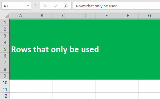
- After the rows are selected to be hidden, the user will only see those not set as hidden. In this way, the rows are limited in Excel.


Example #2 – Restrict Accessing Rows by Protecting the Worksheet
Another simple way of restricting the rows in excel is by protecting the sheet and disabling the feature of allowing the user to select locked cells in excelIn Excel, cells are locked to protect them from unwanted editing, deleting, and overwriting. Locking cells is specifically beneficial in cases where an excel worksheet needs to be shared with several colleagues.read more. This way, we can restrict the user from accessing the restricted rows.
In this method, the user is only restricted from accessing the rows. However, all the rows are still visible to the users.
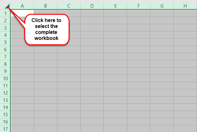
- Step 1: Select the complete workbook.
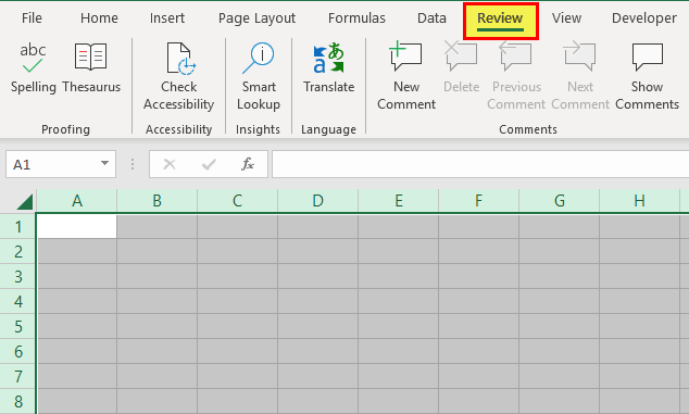
- Step 2: Now, go to the “Review” tab.
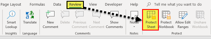
- Step 3: Now, select the option of “Protect Sheet.”
- Step 4: From the options of protecting the sheet, Untick the option “Select locked cells.” By not checking this option, Excel will now not allow the users to select the locked cells.
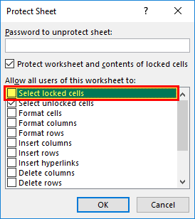
- Step 5: The complete worksheet is locked and cannot be accessed since we have protected the complete worksheet.
- Step 6: Now, we must unprotect the rows or fields that we want the users to have access to. Select the rows that are to be made available.
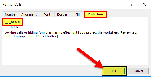
- Step 7: Now, right-click and choose the option of “Format Cells.”
- Step 8: Choose the option to unprotect the range from the “Format CellsFormatting cells is an important technique to master because it makes any data presentable, crisp, and in the user’s preferred format. The formatting of the cell depends upon the nature of the data present.read more” option.
- Step 9: Now, the rows are limited, as only the selected rows are accessible by the user.
Example #3 – Limit Worksheet Rows in Excel with VBA (Scroll Lock)
In this method, the rows are blocked from accessing.
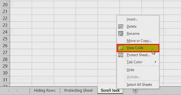
Step 1: Right-click on the sheet name and click “View Code.”
- Step 2: Go to the “View” tab and select the “Properties Window.” You can also use the shortcut key F4 to choose the properties window.

- Step 3: Now, go to the “ScrollArea” and insert the rows to be made available to the user.
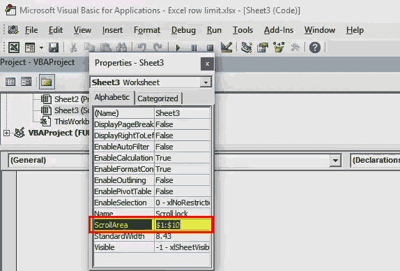
- Step 4: The user can only access the first 10 rows in Excel.

Things to Remember
- By doing the limit of rows in Excel, we only choose to hide the rows that are not yet required.
- When rows are inactive, they are only not available in the current worksheet and can be accessed in a new worksheet.
- Only the current worksheet will be affected if we use the scroll lock option to inactivate some of the rows. Other sheets will not get impacted as the property is only changed for that worksheet, whose code is viewed and then changed.
- The rows number will not get affected, and the rows will not get a reassigned number if any of the rows are hidden. If we have hidden the first 10 rows, this does not mean that the 11th row will get first. The 11th row will remain the 11th row since Excel wants the user to notify that some rows are hidden.
- If we are using the “ScrollArea” option to limit the rows, then this can be changed by the other user as this option to change the scroll option is available to all users as this option does not make the changes protected.
- If we do not want other users to change any of the rules we have created related to the available rows, then we must use the option of “Protect sheet in excelWhen we don’t want any other user to make changes to our worksheet, we can use the Protect worksheet feature in Excel. It can be found in Excel’s Review tab. read more” and then continue with a password.
Recommended Articles
This article is a guide to Excel Rows Limit. Here, we discuss how to limit the rows in Excel using the hide feature, protect the worksheet, and VBA scroll lock, along with practical examples and downloadable templates. You may learn more about Excel from the following articles: –
- Count Rows in ExcelThere are numerous ways to count rows in Excel using the appropriate formula, whether they are data rows, empty rows, or rows containing numerical/text values. Depending on the circumstance, you can use the COUNTA, COUNT, COUNTBLANK, or COUNTIF functions.read more
- VBA Last Row FunctionThe End(XLDown) method is the most commonly used method in VBA to find the last row, but there are other methods, such as finding the last value in VBA using the find function (XLDown).read more
- Remove Blank Rows in Excel
- Row Function Excel Example
Reader Interactions
Содержание
- Insert one or more rows, columns, or cells in Excel for Mac
- Insert rows
- Insert columns
- Insert cells
- Resize a table by adding or removing rows and columns
- Need more help?
- How to Limit Rows and Columns in Excel
- What to Know
- Hide Rows and Columns in Excel
- Unhide Rows and Columns in Excel
- Limit Access to Rows and Columns With VBA
Insert one or more rows, columns, or cells in Excel for Mac
You can insert rows above a selected row and columns to the left of a selected column. Similarly, you can insert blank cells above or to the left of the active cell on a worksheet. Cell references automatically adjust to match the location of the shifted cells.
Insert rows
Select the heading of the row above where you want to insert additional rows.
Tip: Select the same number of rows as you want to insert. For example, to insert five blank rows, select five rows. It’s okay if the rows contain data, because it will insert the rows above these rows.
Hold down CONTROL, click the selected rows, and then on the pop-up menu, click Insert.
Tip: To insert rows that contain data, see Copy and paste specific cell contents.
Insert columns
Select the heading of the column to the right of which you want to insert additional columns.
Tip: Select the same number of columns as you want to insert. For example, to insert five blank columns, select five columns. It’s okay if the columns contain data, because it will insert the columns to the left of these rows.
Hold down CONTROL, click the selected columns, and then on the pop-up menu, click Insert.
Tip: To insert columns that contain data, see Copy and paste specific cell contents.
Insert cells
When you insert blank cells, you can choose whether to shift other cells down or to the right to accommodate the new cells. Cell references automatically adjust to match the location of the shifted cells.
Select the cell, or the range of cells, to the right or above where you want to insert additional cells.
Tip: Select the same number of cells as you want to insert. For example, to insert five blank cells, select five cells.
Hold down CONTROL, click the selected cells, then on the pop-up menu, click Insert.
On the Insert menu, select whether to shift the selected cells down or to the right of the newly inserted cells.
Here’s what happens when you shift cells left:
Here’s what happens when you shift cells down:
Tip: To insert cells that contain data, see Copy and paste specific cell contents.
Источник
Resize a table by adding or removing rows and columns
After you create an Excel table in your worksheet, you can easily add or remove table rows and columns.
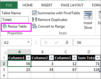
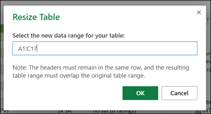
You can use the Resize command in Excel to add rows and columns to a table:
Click anywhere in the table, and the Table Tools option appears.
Click Design > Resize Table.
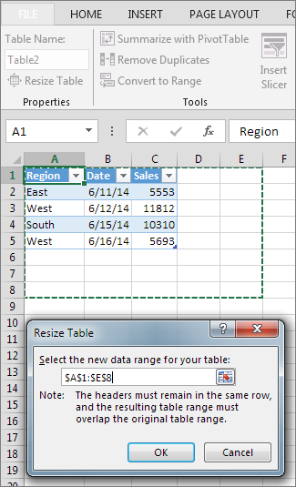
Select the entire range of cells you want your table to include, starting with the upper-leftmost cell.
In the example shown below, the original table covers the range A1:C5. After resizing to add two columns and three rows, the table will cover the range A1:E8.
Tip: You can also click Collapse Dialog  to temporarily hide the Resize Table dialog box, select the range on the worksheet, and then click Expand dialog
  .
.
When you’ve selected the range you want for your table, press OK.
Add a row or column to a table by typing in a cell just below the last row or to the right of the last column, by pasting data into a cell, or by inserting rows or columns between existing rows or columns.
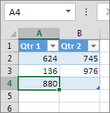
To add a row at the bottom of the table, start typing in a cell below the last table row. The table expands to include the new row. To add a column to the right of the table, start typing in a cell next to the last table column.
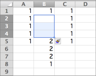
In the example shown below for a row, typing a value in cell A4 expands the table to include that cell in the table along with the adjacent cell in column B.
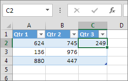
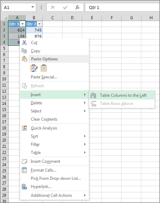
In the example shown below for a column, typing a value in cell C2 expands the table to include column C, naming the table column Qtr 3 because Excel sensed a naming pattern from Qtr 1 and Qtr 2.
To add a row by pasting, paste your data in the leftmost cell below the last table row. To add a column by pasting, paste your data to the right of the table’s rightmost column.
If the data you paste in a new row has as many or fewer columns than the table, the table expands to include all the cells in the range you pasted. If the data you paste has more columns than the table, the extra columns don’t become part of the table—you need to use the Resize command to expand the table to include them.
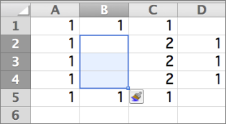
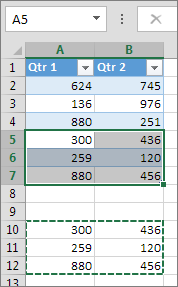
In the example shown below for rows, pasting the values from A10:B12 in the first row below the table (row 5) expands the table to include the pasted data.
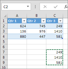
In the example shown below for columns, pasting the values from C7:C9 in the first column to right of the table (column C) expands the table to include the pasted data, adding a heading, Qtr 3.
Use Insert to add a row
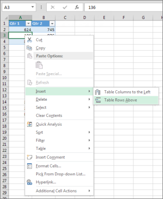
To insert a row, pick a cell or row that’s not the header row, and right-click. To insert a column, pick any cell in the table and right-click.
Point to Insert, and pick Table Rows Above to insert a new row, or Table Columns to the Left to insert a new column.
If you’re in the last row, you can pick Table Rows Above or Table Rows Below.
In the example shown below for rows, a row will be inserted above row 3.
For columns, if you have a cell selected in the table’s rightmost column, you can choose between inserting Table Columns to the Left or Table Columns to the Right.
In the example shown below for columns, a column will be inserted to the left of column 1.
Select one or more table rows or table columns that you want to delete.
You can also just select one or more cells in the table rows or table columns that you want to delete.
On the Home tab, in the Cells group, click the arrow next to Delete, and then click Delete Table Rows or Delete Table Columns.

You can also right-click one or more rows or columns, point to Delete on the shortcut menu, and then click Table Columns or Table Rows. Or you can right-click one or more cells in a table row or table column, point to Delete, and then click Table Rows or Table Columns.
Just as you can remove duplicates from any selected data in Excel, you can easily remove duplicates from a table.
Click anywhere in the table.
This displays the Table Tools, adding the Design tab.
On the Design tab, in the Tools group, click Remove Duplicates.
In the Remove Duplicates dialog box, under Columns, select the columns that contain duplicates that you want to remove.
You can also click Unselect All and then select the columns that you want or click Select All to select all of the columns.
Note: Duplicates that you remove are deleted from the worksheet. If you inadvertently delete data that you meant to keep, you can use Ctrl+Z or click Undo  on the Quick Access Toolbar to restore the deleted data. You may also want to use conditional formats to highlight duplicate values before you remove them. For more information, see Add, change, or clear conditional formats.
Make sure that the active cell is in a table column.
Click the arrow  in the column header.
To filter for blanks, in the AutoFilter menu at the top of the list of values, clear (Select All), and then at the bottom of the list of values, select (Blanks).
Note: The (Blanks) check box is available only if the range of cells or table column contains at least one blank cell.
Select the blank rows in the table, and then press CTRL+- (hyphen).
You can use a similar procedure for filtering and removing blank worksheet rows. For more information about how to filter for blank rows in a worksheet, see Filter data in a range or table.
Select the table, then select Table Design > Resize Table.
Adjust the range of cells the table contains as needed, then select OK.
Important: Table headers can’t move to a different row, and the new range must overlap the original range.
Need more help?
You can always ask an expert in the Excel Tech Community or get support in the Answers community.
Источник
How to Limit Rows and Columns in Excel
Display only what you want to see
What to Know
- To hide certain rows: Select or highlight the rows you want to hide. Right-click a row heading and choose Hide. Repeat for columns.
- To unhide: Right-click the header for the last visible row or column and choose Unhide.
- To temporarily limit range of cells: Right-click sheet tab >View Code >Properties. For ScrollArea, type A1:Z30. Save, close, and reopen Excel.
To help control the size of an Excel worksheet, you can limit the number of columns and rows that a worksheet displays. In this guide, we show you how to hide (and unhide) rows and columns in Excel 2019, Excel 2016, Excel 2013, and Excel for Microsoft 365, as well as how to limit access to rows and columns using Microsoft Visual Basic for Applications (VBA).
Hide Rows and Columns in Excel
An alternative method for restricting the work area of a worksheet is to hide sections of unused rows and columns; they’ll stay hidden even after you close the document. Follow the steps below to hide the rows and columns outside the range A1:Z30.
Open your workbook and select the worksheet you want to hide rows and columns in. Click the header for row 31 to select the entire row.
:max_bytes(150000):strip_icc()/Sites-97f9f6afae9f455b8ca922903c3e054f.jpg)
Press and hold the Shift and Ctrl keys on the keyboard. At the same time, press the down arrow key on the keyboard to select all rows from row 31 to the bottom of the worksheet. Release all the keys.
:max_bytes(150000):strip_icc()/SelectRows-089aa3f6908547dc92c6d18d5cceb581.jpg)
Right-click one of the row headings to open the contextual menu. Select Hide.
:max_bytes(150000):strip_icc()/Hide-7f443bc6033e4d4b98b8702922e7c8db.jpg)
The worksheet now shows only the data in rows 1 through 30.
:max_bytes(150000):strip_icc()/LimitedRows-5d73916e26b9448081cfc254ebeaeaa9.jpg)
Click the header for column AA and repeat steps 2 and 3 (using the right arrow key instead of the down arrow key) to hide all columns after column Z.
:max_bytes(150000):strip_icc()/HideColumns-4bf2226c133e41a39b79a7784007b049.jpg)
Save the workbook; the columns and rows outside the range A1 to Z30 will remain hidden until you unhide them.
You can use the same process to hide any rows or columns you want. Just select the header or headers for the row or column, right-click the header, and select Hide.
Unhide Rows and Columns in Excel
When you want to view the data you hid, you can unhide the rows and columns at any time. Follow these steps to unhide the rows and columns you hid in the previous example.
Open the worksheet you used to hide row 31 and higher and column AA and higher. Click the headers for row 30 (or the last visible row in the worksheet) and the row below it. Right-click the row headers and, from the menu, select Unhide.
:max_bytes(150000):strip_icc()/Unhide-f3e3f2fbeaef478da59ddd8c5b920d8a.jpg)
The hidden rows are restored.
:max_bytes(150000):strip_icc()/Unhidden-c03c6e55715d4f0c9770a11f8ef34c65.jpg)
Now click the headers for column Z (or the last visible column) and the column to the right of it. Right-click the selected column headers and, from the menu, choose Unhide. The hidden columns are restored.
:max_bytes(150000):strip_icc()/ColumnsRestored-d06dd25083b44cf88afb91f689043806.jpg)
Limit Access to Rows and Columns With VBA
You can use Microsoft Visual Basic for Applications (VBA) to temporarily limit the range of usable rows and columns in a worksheet. In this example, you’ll change the properties of a worksheet to limit the number of available rows to 30 and the number of columns to 26.
Changing the scroll area is a temporary measure; it resets each time the workbook is closed and reopened.
Open a blank Excel file. At the bottom of the screen, right-click the Sheet1 sheet tab. From the menu, choose View Code.
:max_bytes(150000):strip_icc()/NewSheet-e1932e0f521b40a580f8f7a7fc7c562a.jpg)
The Visual Basic for Applications (VBA) editor window opens. In the left rail, locate the Properties section.
:max_bytes(150000):strip_icc()/VBA-0ae3957795f04c6181fbc39c20f2edb1.jpg)
Under Properties,in the right column of the ScrollArea row, click the empty box and type A1:Z30.
:max_bytes(150000):strip_icc()/A1Z30-fbba47ba3f2847ae94c6fae7a77b1193.jpg)
Select File > Save and save your workbook as you normally would. Select File > Close and Return to Microsoft Excel.
:max_bytes(150000):strip_icc()/Save-e853356887ce44f1b6a05f4e26e0c318.jpg)
To make sure your change is applied, perform this test. In your worksheet, try to scroll past row 30 or column Z. If the change has been applied, Excel bounces you back to the selected range and you’re unable to edit cells outside that range.
:max_bytes(150000):strip_icc()/TestRange-a77a1c94b58a42a2b257ec3e6248d800.jpg)
To remove the restrictions, access VBA again and delete the ScrollArea range.
Microsoft says that the maximum size of a single Excel spreadsheet is 1,048,576 rows by 16,384 columns. The maximum row height is 409 points, and the maximum column width is 255 characters.
Источник
This post will guide you how to limit rows and columns in an Excel Worksheet. How do I limit the number of rows and columns in an Excel Spreadsheet.
- Limit Rows and Columns with VBA
- Limit Rows and Columns with Hiding Rows and Columns
- Video: Limit Rows and Columns
Limit Rows and Columns with VBA
Assuming that you have a worksheet, and you want to allow other people to edit your worksheet only, but you do not want them to add more rows or columns. So you need to limit the number of rows and columns in your worksheet. You can temporarily prevent other people from scrolling below a certain row and column. And how to disable scrolling below a specific row and column, you can use the Scroll Area property of the worksheet to limit the range of usable rows and columns. Just do the following steps:
#1 right click on your worksheet tab at the bottom of your worksheet. And click View Code menu from the popup menu list. And the Visual Basic for Applications window will open.
#2 click View Menu in the Visual Basic for Applications window, and then click Properties Window menu from the drop down menu list. And the Properties window will be shown.
#3 Find the Scroll Area property in the list of worksheet properties.
#4 click in the empty box to the right of the Scroll Area label. And type the range of cells that you want to display.
#5 press Ctrl + S keys and save the worksheet. And then close the Visual Basic for Applications window and return the worksheet.
#6 you will be unable to scroll past the row number you typed into the scroll Area text box. And all other rows are also be locked.
You can also try to hide all other rows and columns to achieve the same result of limiting rows and columns in your worksheet. For example, If you need to hide the rows and columns outside the range A1:C4, just do the following steps:
#1 click the row 5 to select the entire row.
#2 press Shift + Ctrl + Down Arrow keys in your keyboard, to select all rows from row 5 to the bottom of the worksheet.
#3 right click on the selected rows and choose Hide from the popup menu list.
#4 click on the Column D to select the entire column. And press Shift + Ctrl + right Arrow keys in your keyboard, to select all rows from row 5 to the bottom of the worksheet. Then repeat step 3 to hide all columns after column C.
#5 You will see that all rows and columns outside the range A1:C4 will be hidden.
Video: Limit Rows and Columns
Display only what you want to see
Updated on September 26, 2022
What to Know
- To hide certain rows: Select or highlight the rows you want to hide. Right-click a row heading and choose Hide. Repeat for columns.
- To unhide: Right-click the header for the last visible row or column and choose Unhide.
- To temporarily limit range of cells: Right-click sheet tab > View Code > Properties. For ScrollArea, type A1:Z30. Save, close, and reopen Excel.
To help control the size of an Excel worksheet, you can limit the number of columns and rows that a worksheet displays. In this guide, we show you how to hide (and unhide) rows and columns in Excel 2019, Excel 2016, Excel 2013, and Excel for Microsoft 365, as well as how to limit access to rows and columns using Microsoft Visual Basic for Applications (VBA).
Hide Rows and Columns in Excel
An alternative method for restricting the work area of a worksheet is to hide sections of unused rows and columns; they’ll stay hidden even after you close the document. Follow the steps below to hide the rows and columns outside the range A1:Z30.
-
Open your workbook and select the worksheet you want to hide rows and columns in. Click the header for row 31 to select the entire row.
-
Press and hold the Shift and Ctrl keys on the keyboard. At the same time, press the down arrow key on the keyboard to select all rows from row 31 to the bottom of the worksheet. Release all the keys.
-
Right-click one of the row headings to open the contextual menu. Select Hide.
-
The worksheet now shows only the data in rows 1 through 30.
-
Click the header for column AA and repeat steps 2 and 3 (using the right arrow key instead of the down arrow key) to hide all columns after column Z.
-
Save the workbook; the columns and rows outside the range A1 to Z30 will remain hidden until you unhide them.
You can use the same process to hide any rows or columns you want. Just select the header or headers for the row or column, right-click the header, and select Hide.
Unhide Rows and Columns in Excel
When you want to view the data you hid, you can unhide the rows and columns at any time. Follow these steps to unhide the rows and columns you hid in the previous example.
-
Open the worksheet you used to hide row 31 and higher and column AA and higher. Click the headers for row 30 (or the last visible row in the worksheet) and the row below it. Right-click the row headers and, from the menu, select Unhide.
-
The hidden rows are restored.
-
Now click the headers for column Z (or the last visible column) and the column to the right of it. Right-click the selected column headers and, from the menu, choose Unhide. The hidden columns are restored.
Limit Access to Rows and Columns With VBA
You can use Microsoft Visual Basic for Applications (VBA) to temporarily limit the range of usable rows and columns in a worksheet. In this example, you’ll change the properties of a worksheet to limit the number of available rows to 30 and the number of columns to 26.
Changing the scroll area is a temporary measure; it resets each time the workbook is closed and reopened.
-
Open a blank Excel file. At the bottom of the screen, right-click the Sheet1 sheet tab. From the menu, choose View Code.
-
The Visual Basic for Applications (VBA) editor window opens. In the left rail, locate the Properties section.
-
Under Properties,in the right column of the ScrollArea row, click the empty box and type A1:Z30.
-
Select File > Save and save your workbook as you normally would. Select File > Close and Return to Microsoft Excel.
-
To make sure your change is applied, perform this test. In your worksheet, try to scroll past row 30 or column Z. If the change has been applied, Excel bounces you back to the selected range and you’re unable to edit cells outside that range.
-
To remove the restrictions, access VBA again and delete the ScrollArea range.
FAQ
-
What is the maximum limit of rows in Excel?
Microsoft says that the maximum size of a single Excel spreadsheet is 1,048,576 rows by 16,384 columns. The maximum row height is 409 points, and the maximum column width is 255 characters.
-
How do I permanently set row and column limits in Excel?
If you want to set a hard limit to columns or rows in an Excel spreadsheet (i.e. set it up so no additional rows or columns can be added past that set limit), unfortunately you can’t. There’s currently no menu option to prevent yourself or other users from adding more rows or columns you may not want. However, you can manually delete unwanted rows and columns by right-clicking the selected row(s) or column(s) and selecting Delete.
Thanks for letting us know!
Get the Latest Tech News Delivered Every Day
Subscribe
Resize a table by adding or removing rows and columns
Excel for Microsoft 365 Excel for the web Excel 2021 Excel 2019 Excel 2016 Excel 2013 Excel 2010 Excel 2007 More…Less
After you create an Excel table in your worksheet, you can easily add or remove table rows and columns.
You can use the Resize command in Excel to add rows and columns to a table:
-
Click anywhere in the table, and the Table Tools option appears.
-
Click Design > Resize Table.

-
Select the entire range of cells you want your table to include, starting with the upper-leftmost cell.
In the example shown below, the original table covers the range A1:C5. After resizing to add two columns and three rows, the table will cover the range A1:E8.
Tip: You can also click Collapse Dialog
to temporarily hide the Resize Table dialog box, select the range on the worksheet, and then click Expand dialog . -
When you’ve selected the range you want for your table, press OK.
Add a row or column to a table by typing in a cell just below the last row or to the right of the last column, by pasting data into a cell, or by inserting rows or columns between existing rows or columns.
Start typing
-
To add a row at the bottom of the table, start typing in a cell below the last table row. The table expands to include the new row. To add a column to the right of the table, start typing in a cell next to the last table column.
In the example shown below for a row, typing a value in cell A4 expands the table to include that cell in the table along with the adjacent cell in column B.
In the example shown below for a column, typing a value in cell C2 expands the table to include column C, naming the table column Qtr 3 because Excel sensed a naming pattern from Qtr 1 and Qtr 2.
Paste data
-
To add a row by pasting, paste your data in the leftmost cell below the last table row. To add a column by pasting, paste your data to the right of the table’s rightmost column.
If the data you paste in a new row has as many or fewer columns than the table, the table expands to include all the cells in the range you pasted. If the data you paste has more columns than the table, the extra columns don’t become part of the table—you need to use the Resize command to expand the table to include them.
In the example shown below for rows, pasting the values from A10:B12 in the first row below the table (row 5) expands the table to include the pasted data.
In the example shown below for columns, pasting the values from C7:C9 in the first column to right of the table (column C) expands the table to include the pasted data, adding a heading, Qtr 3.
Use Insert to add a row
-
To insert a row, pick a cell or row that’s not the header row, and right-click. To insert a column, pick any cell in the table and right-click.
-
Point to Insert, and pick Table Rows Above to insert a new row, or Table Columns to the Left to insert a new column.
If you’re in the last row, you can pick Table Rows Above or Table Rows Below.
In the example shown below for rows, a row will be inserted above row 3.
For columns, if you have a cell selected in the table’s rightmost column, you can choose between inserting Table Columns to the Left or Table Columns to the Right.
In the example shown below for columns, a column will be inserted to the left of column 1.
-
Select one or more table rows or table columns that you want to delete.
You can also just select one or more cells in the table rows or table columns that you want to delete.
-
On the Home tab, in the Cells group, click the arrow next to Delete, and then click Delete Table Rows or Delete Table Columns.
You can also right-click one or more rows or columns, point to Delete on the shortcut menu, and then click Table Columns or Table Rows. Or you can right-click one or more cells in a table row or table column, point to Delete, and then click Table Rows or Table Columns.
Just as you can remove duplicates from any selected data in Excel, you can easily remove duplicates from a table.
-
Click anywhere in the table.
This displays the Table Tools, adding the Design tab.
-
On the Design tab, in the Tools group, click Remove Duplicates.
-
In the Remove Duplicates dialog box, under Columns, select the columns that contain duplicates that you want to remove.
You can also click Unselect All and then select the columns that you want or click Select All to select all of the columns.
Note: Duplicates that you remove are deleted from the worksheet. If you inadvertently delete data that you meant to keep, you can use Ctrl+Z or click Undo on the Quick Access Toolbar to restore the deleted data. You may also want to use conditional formats to highlight duplicate values before you remove them. For more information, see Add, change, or clear conditional formats.
-
Make sure that the active cell is in a table column.
-
Click the arrow
in the column header. -
To filter for blanks, in the AutoFilter menu at the top of the list of values, clear (Select All), and then at the bottom of the list of values, select (Blanks).
Note: The (Blanks) check box is available only if the range of cells or table column contains at least one blank cell.
-
Select the blank rows in the table, and then press CTRL+- (hyphen).
You can use a similar procedure for filtering and removing blank worksheet rows. For more information about how to filter for blank rows in a worksheet, see Filter data in a range or table.
-
Select the table, then select Table Design > Resize Table.
-
Adjust the range of cells the table contains as needed, then select OK.
Important: Table headers can’t move to a different row, and the new range must overlap the original range.
Need more help?
You can always ask an expert in the Excel Tech Community or get support in the Answers community.
See Also
How can I merge two or more tables?
Create an Excel table in a worksheet
Use structured references in Excel table formulas
Format an Excel table