
Show or hide gridlines on a worksheet
Excel for Microsoft 365 Excel for Microsoft 365 for Mac Excel for the web Excel 2021 Excel 2021 for Mac Excel 2019 Excel 2019 for Mac Excel 2016 Excel 2016 for Mac Excel 2013 Excel 2010 Excel 2007 Excel for Mac 2011 Excel Starter 2010 More…Less
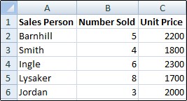
Gridlines are the faint lines that appear between cells on a worksheet.
When working with gridlines, consider the following:
-
By default, gridlines are displayed in worksheets using a color that is assigned by Excel. If you want, you can change the color of the gridlines for a particular worksheet by clicking Gridline color under Display options for this worksheet (File tab, Options, Advanced category).
-
People often confuse borders and gridlines in Excel. Gridlines cannot be customized in the same manner that borders can. If you want to change the width or other attributes of the lines for a border, see Apply or remove cell borders on a worksheet.
-
If you apply a fill color to cells on your worksheet, you won’t be able to see or print the cell gridlines for those cells. To see or print the gridlines for these cells, remove the fill color by selecting the cells, and then click the arrow next to Fill Color
 (Home tab, Font group), and To remove the fill color, click No Fill.
Note: You must remove the fill completely. If you change the fill color to white, the gridlines will remain hidden. To keep the fill color and still see lines that serve to separate cells, you can use borders instead of gridlines. For more information, see Apply or remove cell borders on a worksheet.
-
Gridlines are always applied to the whole worksheet or workbook, and can’t be applied to specific cells or ranges. If you want to apply lines selectively around specific cells or ranges of cells, you should use borders instead of, or in addition to, gridlines. For more information, see Apply or remove cell borders on a worksheet.
 (Home tab, Font group), and To remove the fill color, click No Fill.
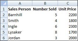
If the design of your workbook requires it, you can hide the gridlines:
-
Select one or more worksheets.
Tip: When multiple worksheets are selected, [Group] appears in the title bar at the top of the worksheet. To cancel a selection of multiple worksheets in a workbook, click any unselected worksheet. If no unselected sheet is visible, right-click the tab of a selected sheet, and then click Ungroup Sheets.
-
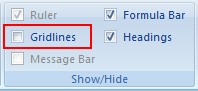
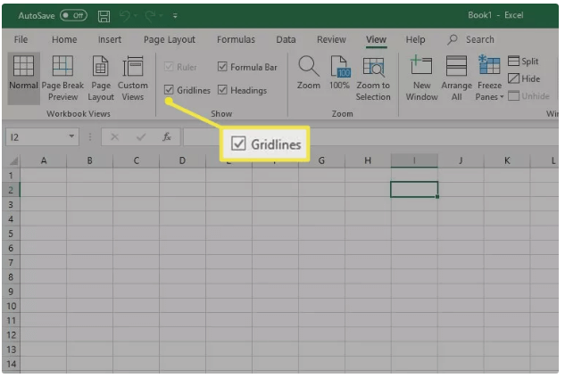
In Excel 2007: On the View tab, in the Show/Hide group, clear the Gridlines check box.
In all other Excel versions: On the View tab, in the Show group, clear the Gridlines check box.
If the gridlines on your worksheet are hidden, you can follow these steps to show them again.
-
Select one or more worksheets.
Tip: When multiple worksheets are selected, [Group] appears in the title bar at the top of the worksheet. To cancel a selection of multiple worksheets in a workbook, click any unselected worksheet. If no unselected sheet is visible, right-click the tab of a selected sheet, and then click Ungroup Sheets.
-
Excel 2007: On the View tab, in the Show/Hide group, select the Gridlines check box.
All other Excel versions: On the View tab, in the Show group, select the Gridlines check box.
Note: Gridlines do not print by default. For gridlines to appear on the printed page, select the Print check box under Gridlines (Page Layout tab, Sheet Options group).
-
Select the worksheet.
-
Click the Page Layout tab.
-
To show gridlines: Under Gridlines, select the View check box.
To hide gridlines: Under Gridlines, clear the View check box.
Follow these steps to show or hide gridlines.
-
Click the sheet.
-
To show gridlines: On the Layout tab, under View, select the Gridlines check box.
Note: Gridlines cannot be customized. To change the width, color, or other attributes of the lines around cells, use border formatting.
To hide gridlines: On the Layout tab, under View, clear the Gridlines check box.
Gridlines are used to distinguish cells on a worksheet. When working with gridlines, consider the following:
-
By default, gridlines are displayed on worksheets using a color that is assigned by Excel. If you want, you can change the color of the gridlines for a particular worksheet.
-
People often confuse borders and gridlines in Excel. Gridlines cannot be customized in the same way that borders can.
-
If you apply a fill color to cells on a worksheet, you won’t be able to see or print the cell gridlines for those cells. To see or print the gridlines for these cells, you must remove the fill color. Keep in mind that you must remove the fill entirely. If you simply change the fill color to white, the gridlines will remain hidden. To retain the fill color and still see lines that serve to separate cells, you can use borders instead of gridlines.
-
Gridlines are always applied to the entire worksheet or workbook and can’t be applied to specific cells or ranges. If you want to selectively apply lines around specific cells or ranges of cells, you should use borders instead of, or in addition to, gridlines.
You can either show or hide gridlines on a worksheet in Excel for the web.
On the View tab, in the Show group, select the Gridlines check box to show gridlines, or clear the check box to hide them.
Excel for the web works seamlessly with the Office desktop programs. Try or buy the latest version of Office now.
See Also
Show or hide gridlines in Word, PowerPoint, and Excel
Print gridlines in a worksheet
Need more help?
Want more options?
Explore subscription benefits, browse training courses, learn how to secure your device, and more.
Communities help you ask and answer questions, give feedback, and hear from experts with rich knowledge.
- Select the worksheet.
- Click the Page Layout tab.
- To show gridlines: Under Gridlines, select the View check box. To hide gridlines: Under Gridlines, clear the View check box.
Contents
- 1 How do I get rid of gridlines in Excel?
- 2 How do I make an Excel sheet blank?
- 3 How do I get rid of lines in sheets?
- 4 How do I hide grid lines in sheets?
- 5 How do I make a spreadsheet white?
- 6 How do you remove gridlines from specific cells in sheets?
- 7 How do I hide rows in Google Sheets?
- 8 How do you make a table without vertical lines in Google Docs?
- 9 How do I conditionally hide rows in Google Sheets?
- 10 What is the shortcut to hide rows in Google Sheets?
- 11 How do you add lines in sheets?
- 12 How do you start a new line within a cell in Excel?
- 13 How do I make multiple lines in one cell in Google Sheets?
- 14 How do I make my table lines invisible in Word?
- 15 How do you get rid of lines in Google Docs?
How do I get rid of gridlines in Excel?
How to Remove Excel Gridlines. The easiest way to remove gridlines in Excel is to use the Page Layout tab. Click the Page Layout tab to expand the page layout commands and then go to the Gridlines section. Below Gridlines, uncheck the view box.
Open a new, blank workbook
- Click the File tab.
- Click New.
- Under Available Templates, double-click Blank Workbook. Keyboard shortcut To quickly create a new, blank workbook, you can also press CTRL+N.
How do I get rid of lines in sheets?
Start by opening your Google Sheet spreadsheet and clicking “View” from the menu bar. From the “View” menu, select the “Gridlines” option to uncheck it. Once that’s unchecked, all gridlines between cells across your spreadsheet will disappear from view.
How do I hide grid lines in sheets?
- Select the worksheet.
- Click the Page Layout tab.
- To show gridlines: Under Gridlines, select the View check box. To hide gridlines: Under Gridlines, clear the View check box.
How do I make a spreadsheet white?
Show / hide gridlines in Excel by changing the fill color
- Select the necessary range or the entire spreadsheet.
- Go to the Font group on the HOME tab and open the Fill Color drop-down list.
- Choose the white color from the list to remove gridlines.
How do you remove gridlines from specific cells in sheets?
Below are the steps to hide the gridlines in Google sheets worksheet:
- Select the worksheet in which you want to hide the gridlines.
- Click the View button in the menu.
- In the drop-down that opens, click the Gridlines options. This will uncheck the Gridlines options.
How do I hide rows in Google Sheets?
How to hide rows in Google Sheets on a computer
- Open the Google Sheet you want to edit on your Mac or PC.
- Select the row you want to hide.
- Right-click the selected row and choose Hide row from the menu that opens. Two arrows will appear in place of the hidden row.
How do you make a table without vertical lines in Google Docs?
First, highlight the upper row of cells, click the “Borders” icon and select no top border. Next, highlight the left column of cells, click the “Borders” icon and select no left border. Highlight the bottom row and set it to no bottom border, and then select the far right column and choose no right border.
How do I conditionally hide rows in Google Sheets?
In Google Docs, open a spreadsheet, select a group of cells, and click the icon to change the cell background. Select ‘Change with rules…’ and add your conditional formatting preferences. To hide a row or column, select a set of rows or columns, right click, and choose ‘Hide’.
What is the shortcut to hide rows in Google Sheets?
1. Click or tap on a column or row to select it. 2. Press Ctrl+Alt+0 (zero) to hide a column, or press Ctrl+Alt+9 to hide a row.
How do you add lines in sheets?
Edit data in a cell
- Open a spreadsheet in Google Sheets.
- Click a cell that’s empty, or double-click a cell that isn’t empty.
- Start typing.
- Optional: To add another line within a cell, press ⌘ + Enter on a Mac or Ctrl + Enter on Windows.
- When you’re done, press Enter.
How do you start a new line within a cell in Excel?
Start a new line of text inside a cell in Excel
- Double-click the cell in which you want to insert a line break.
- Click the location inside the selected cell where you want to break the line.
- Press Alt+Enter to insert the line break.
How do I make multiple lines in one cell in Google Sheets?
When you select a cell in Google Sheets, you can right click to add a new row.
- Right-click on a selected cell.
- Choose “Insert Row” from the pop-up menu.
- Click and hold your mouse on the number to the left of the row where you want to add more rows.
How do I make my table lines invisible in Word?
Hover your mouse over the table until the table move handle displays in the upper left corner and then click this handle to select the entire table. Click “Table Tools,” select “Design,” click the arrow on the “Borders” button and then select “No Borders.” This hides the borders for the entire table.
How do you get rid of lines in Google Docs?
Hover over Table in the dropdown menu that appears. Now, select the table size (column x row dimensions) and click to confirm. You should see the table in your document. If you right-click the table, you’ll see options such as Delete row, Delete column, Delete table, Distribute rows, Distribute columns, and so on.
Does your gridline missing in Excel worksheet? Due to this, are you facing difficulty in reading data across the rows?
Gridlines are actually very important in an Excel worksheet as it works like a cell divider. These gridlines help in the easy distinguishing of cells from each other so that the data will look more legible.
So if you are facing missing gridlines in Excel worksheet then don’t get tensed because it’s possible to get them back.
For this, I have outlined some best tricks to solve the mystery of gridlines missing in Excel worksheet.
Here are the following fixes that you must try to fix gridlines missing in Excel worksheet.
1. Best Software To Fix Missing Gridlines In Excel Worksheet
2. Set The Default Color Of Gridlines
3. Remove White Borders
4. Avoid Color Overlay
5. Remove Conditional Formatting
6. Hide Gridlines Of Rows and Columns
7. Turn Gridlines On/Off For Entire Worksheet
Trick 1: Best Software To Fix Excel Missing Gridlines Issue
Mostly this type of missing data or damaged worksheet issue raises when the corruption issue hits your Excel sheet.
So, the first solution which I want to recommend is repairing your corrupt Excel file. For this, the best-recommended solution is using Excel Repair software.
It is the best tool for the recovery of corrupt Excel workbook data and to avoid permanent data loss situations.
To fix corrupt XLS and XLSX file you can go with this professional recommended Excel File Repair software. This is the best tool that helps you to repair and recover corrupted, damaged, and inaccessible data in XLS and XLSX files.
* Free version of the product only previews recoverable data.
Why To Choose Excel File Repair Software?
- Completely preserve entire worksheet properties like freeze panes, split, gridlines, formula bar, and cell formatting.
- Fix all types of Excel corruption errors.
- Shows real-time preview of all the recoverable items from your corrupt xlsx/xls files before starting up the recovery procedure.
- Does easy recovery of all your Excel workbook tables, sorts, and filters, chart sheets, formulas, cell comments, charts, images, etc.
- Well, compatibility and support for both Mac/Windows.
- Repair single and multiple XLSX/ XLS files in one go.
- Well support for all MS Excel versions: 2019/ 2016/ 2013/ 2010/ 2007/ 2003 / 2000.
Steps To Utilize Excel File Repair Software:
2. Set The Default Color Of Gridlines
By default, Excel gives the greyish color of gridlines. So you need to get ensure that the color won’t get changed to white.
The reason behind this is, white gridlines won’t appear on white background. Here are the steps that you need to follow for changing the grid color back to the default one:
1: Go to the File -> Options.
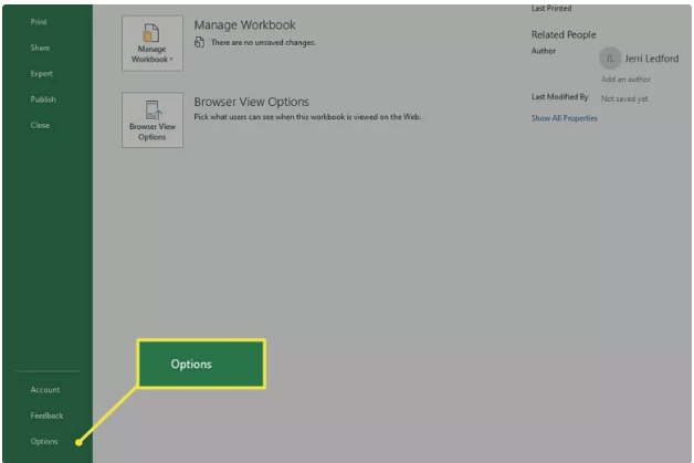
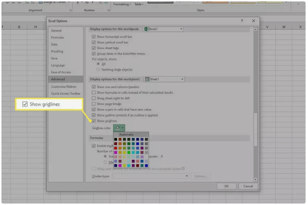
2: Now hit the “Advanced” tab and then scroll down in the section “Display options for this worksheet”.

3: Now hit the drop-down arrow sign present next to the gridlines color option. After that from the opened box of colors choose the automatic option or else you can select any other colors also.
See here from this box, you can choose different types of colors if you wish.
3. Remove White Borders
Check whether your gridlines is having the right property set assigned or not. Besides this whether it is marked for visibility or not.
Chances are also that you are getting these missing gridlines in Excel issue because of the white-colored cell borders. So you have to remove the cell borders to fix this issue.
1: Hit the “Ctrl + A” to choose entire cells. Make a right-tap over the “Format Cells” option.

2: Tap to the “Border” tab and then get ensure that none of the borders are in the active status.
4. Avoid Color Overlay
Most of the time we use different colors to highlight a particular set of data. When colors get covered, gridlines go hidden under them.
If none of the colors are appearing then it may have a chance that the color which is selected for the overlay is the white one.
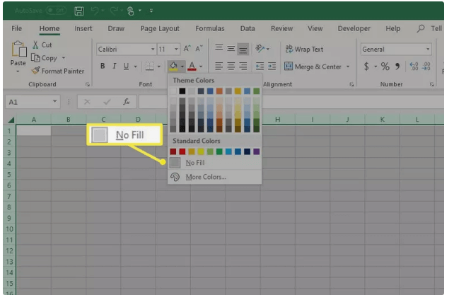
Step 1: Hit the Ctrl + A button to choose entire cells.

Step 2: Tap to the Home tab. Now from the “color fill” option choose “No Fill”.
5. Remove Conditional Formatting
If some type of conditional formatting is applied on the worksheet for hiding worksheet gridlines.
Follow this step: Home -> Styles -> Conditional Formatting -> Clear Rules
NOTE:
By choosing the clearing rules option you are clearing the entire set of rules along with the one you are willing to remove. So it will be better if you manage rules and extract from the detail whether there are some settings to remove particular formattings.
6. Hide Gridlines Of Rows and Columns
In some cases, you want to remove certain sections of gridlines to give visual emphasis to the viewers.
- Select the cells group from which you are willing to remove gridlines.
- Make a right-click over the highlighted cells and then choose Format Cells options. Press the Ctrl+1 button to get into the menu section.

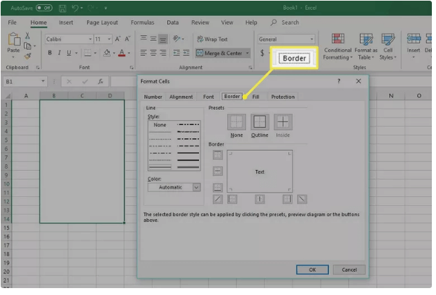
- In the opened dialog box of Format Cells go to the Border tab.
- Choose the white color from the drop-down menu. After that choose the Inside and Outside option from the Presets.

- Hit the OK button to make a confirmation about your selections.
7. Turn Gridlines On/Off For Entire Worksheet
If you are having a spreadsheet in which gridlines are removed or it is made invisible. Mainly there are two options to easily restore gridlines of the entire worksheet.
- Open Excel spreadsheet from which gridlines are removed.
- You have to select more than one worksheet. After that press the CTRL button of your keyboard to choose related sheets from the workbook bottom.
- Choose the View tab and after that choose the Gridline option for restoring all the gridlines.
- Besides this, choose Page Layout and then from the Gridlines settings choose the view tab.

FAQ (Frequently Asked Question):
Why Is Excel Not Printing All Gridlines?
If the gridlines won’t appear in your print preview or meanwhile the printout process then probably the reason is enabled “Draft quality” feature of the printer.
This feature is mainly used for saving the ink and removing gridlines like thing.
- For disabling this feature, follow this path: File > Print > Page Setup.
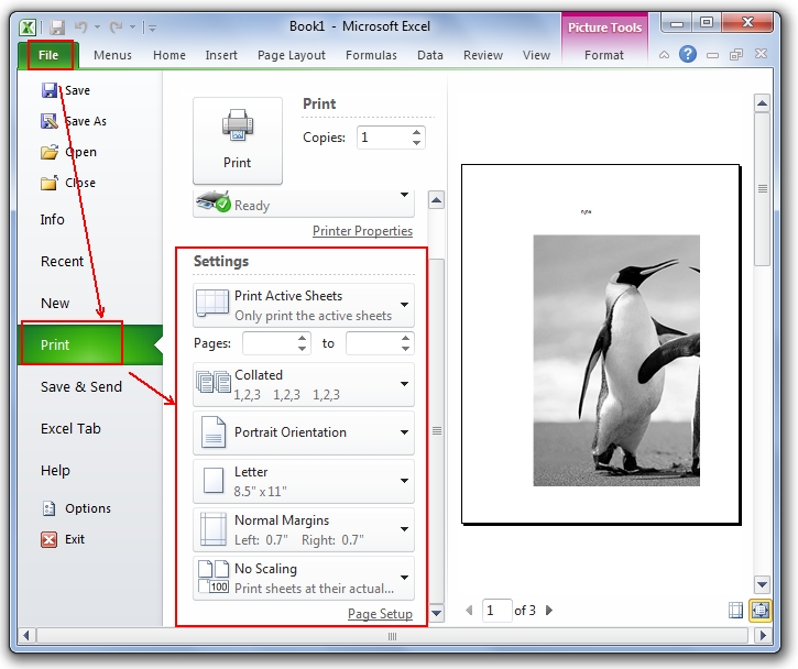
- Now within the page setup switch to the sheet From the print section uncheck the “draft quality” option.

In this way, you can fix the issue of missing gridlines in Excel when printing.
How Do I Make Grid Lines Visible In Excel After Fill Color?
Excel gridlines appear in worksheets by using the default color set in the automatic. Well to make gridlines visible you can change their color. Here are the procedures that you need to use.
- Choose the worksheets of which you need to modify gridline color.
- Tap to the File> Excel > Options.
- Go to the Advanced category and then from the Display options for this worksheet section, choose the Show gridlines check box.
- Now from the Gridline color box, choose the color of your choice.
Tip: To get back the gridlines to the default color, click Automatic.
How To Make Gridlines Darker In Excel?
Usually, Excel applies just a thin line style when you add one outer cell of the gridline or border.
In order to modify the width of gridlines in Excel, follow down the steps:
- Choose the cells in which you want to maximize the gridline width.
- Make a right-click over your selected cells and then choose Format Cells option.
- In the opened window of format, cells choose the Border tab.
- If you want a continuous line, then select the thicker pattern from the opened Line dialog box.
- Within the Presets section, choose the existing border type.
- You can see the new border pattern within the preview option.
- Hit the ok.
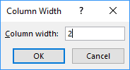
How Do I Change The Grid Size In Excel?
To change the width of grid in the worksheet, you have to follow down the given steps:
- Make a tap over the top-left corner of your Excel spreadsheet. This will select the entire cells in your Excel workbook.
- Right-click over any of the columns and then choose Column Width… from the opened popup menu.

- Within the opened dialog box assign the width size, you want to keep and then hit the OK button.
Conclusion
So for the next time when you face this issue of missing gridlines in Excel at least, you know very well what you have to do.
Besides this, remember one thing that setting is applied to only one sheet in a single piece of time.
Follow the given steps carefully and if you are a novice user then make use of the automatic Excel File Repair tool to resolve gridlines won’t appear in Excel issues.
If, in case you have any additional questions to ask regarding xlsx/xls file recovery, then visit my Repair MS Excel Facebook, Twitter page.


Priyanka is an entrepreneur & content marketing expert. She writes tech blogs and has expertise in MS Office, Excel, and other tech subjects. Her distinctive art of presenting tech information in the easy-to-understand language is very impressive. When not writing, she loves unplanned travels.
See all How-To Articles
This tutorial demonstrates how to draw lines in Excel and Google Sheets.
Draw Lines in Excel
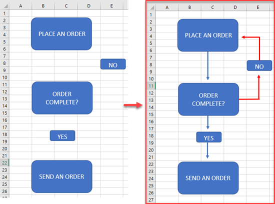
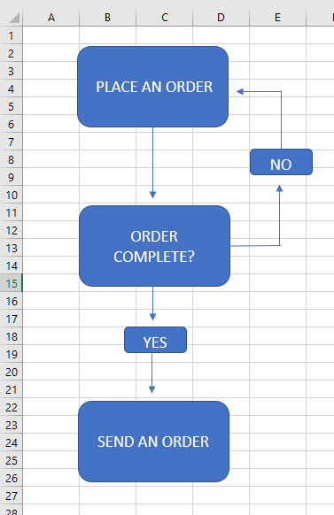
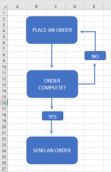
Say you have shapes in your sheet that you want to connect with lines.
- To draw lines, in the Ribbon, click on Insert > Shapes > Lines.
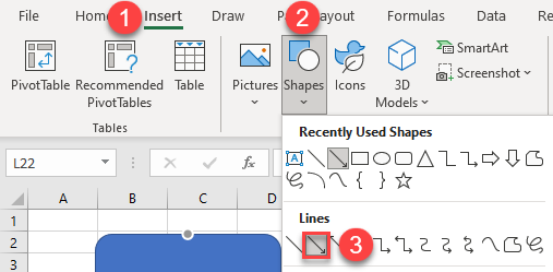
- When the cursor changes to a plus sign, you can start to draw lines.
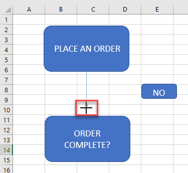
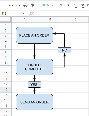
As a result, the lines are added to your sheet.
Change the Line Weight
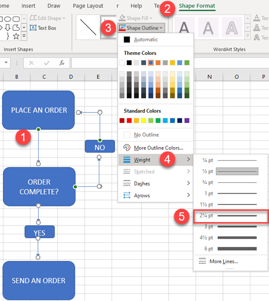
If you want, you can change the lines’ properties, such as color, weight, and style. To change the weight of the lines, follow these steps:
First, select the lines for which you want to change the color. Then, in the Ribbon, click on Shape Format > Shape Outline > Weight. Finally, choose the desired line weight.
As a result, the weight of the selected lines is changed.
Change the Line Color
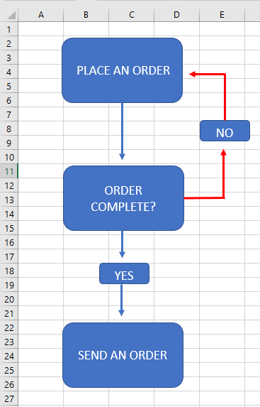
To change the color of the lines, select the lines you want to change. Then, in the Ribbon, click on the Shape Format > Shape Outline. Choose a color.
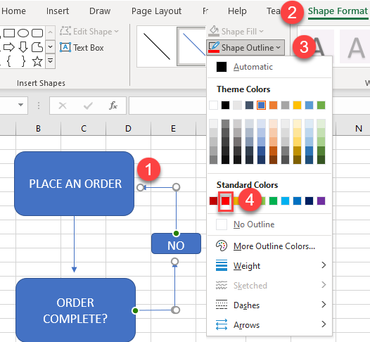
As a result, the color of the selected lines is changed.
Draw Lines in Google Sheets
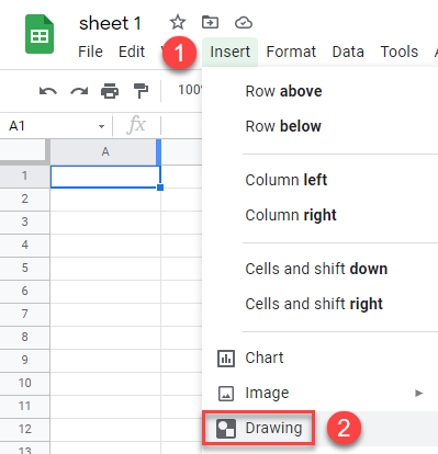
- To draw lines in Google Sheets, in the Menu, click on the Insert, and in the drop-down menu, choose Drawing.
- The Drawing window opens. In the menu, click on the Line icon and choose the line type.
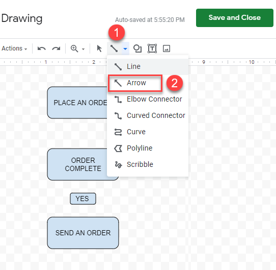
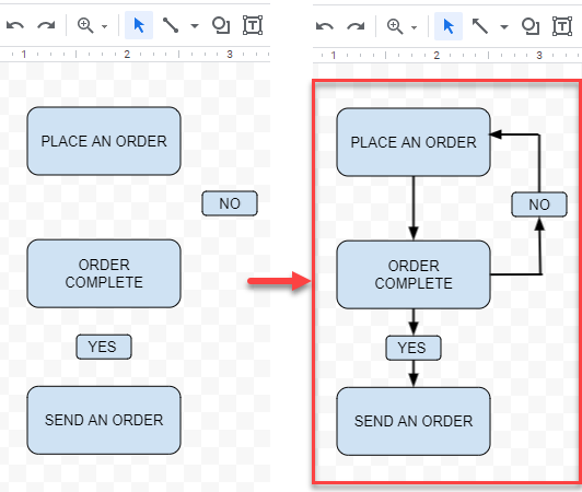
- Use the cursor to draw your lines.
Change Line Weight in Google Sheets
You can also change the properties of the lines, such as color, style, and weight. To change the weight of the lines, follow these steps:
- Select the lines you want to change.
- Then in the Toolbar, click on the Weight icon.
- From the drop-down menu, choose the desired weight of the line.
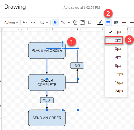
As a result, the weight of the selected lines is changed.
![]()
Download Article
![]()
Download Article
Grid lines, which are the faint lines that divide cells on a worksheet, are displayed by default in Microsoft Excel. You can enable or disable them by worksheet, and even choose to see them on printed pages. Gridlines are different than cell borders, which you can add to cells and ranges and customize with line styles and colors. This wikiHow article will show you how to show gridlines in your Excel worksheet, both on the screen and printed, as well as how to add cell borders to make your data stand out.
Things You Should Know
- On Windows, open your Excel sheet. Go to File > Options > Advanced > «Display options for this worksheet». Choose your worksheet and select «Show gridlines.»
- On Mac, open your Excel sheet. Click the Page Layout tab. Find the «Gridlines» panel and check the «View» box.
- Add borders to cells in both OS’s by selecting your cells and clicking Home. Click the arrow next to the Borders icon and choose a style.
-
1
Open the workbook you want to edit. Gridlines always appear on worksheets by default, but you can enable or disable them for any individual worksheet in your settings.
- If the issue is that you can see gridlines on your worksheet but aren’t seeing them on printed pages, you can just enable gridlines when printing. Skip to Step 8 to learn how.
- If you see gridlines on the page but want to add more obvious borders around certain cells or ranges, see Adding Cell Borders in Windows and macOS.
-
2
Click the File menu and select Options. The Excel Options window will expand.
Advertisement
-
3
Click the Advanced tab. It’s in the left panel.
-
4
Scroll down to the «Display options for this worksheet» area. It’s in the right panel just after the «Display options for this workbook» group.
-
5
Select the sheet that doesn’t have gridlines from the «Display options for this worksheet» menu. If you already see the name of the active worksheet here, you can skip this step.
-
6
Check the box next to «Show gridlines.» If gridlines were hidden, the checkbox would be blank. Clicking the box re-enables gridlines.
- If there was already a check next to «Show gridlines» but you don’t see lines on your sheet, the color may be too light. Click the «Gridline color» menu to choose a darker gray color.
-
7
Click OK. Gridlines are now visible on your worksheet.
-
8
Show gridlines when printing (optional). Gridlines, by default, do not appear on printed versions of your worksheet. If you want to see gridlines when you print, you’ll need to enable them in your Page Setup options. Here’s how:
- Click the name of the sheet you want to print at the bottom of your workbook.
- Click the Page Layout tab at the top.
- Click the small arrow at the bottom-right corner of the «Page Setup» panel in the toolbar.
- Click the Sheet tab.
- Check the box next to «Gridlines» under «Print.»
- Click OK. Now when you print this sheet, gridlines will appear on each page.


Advertisement
-
1
Open the workbook you want to edit. Gridlines always appear on worksheets by default, but you can enable or disable them for any individual worksheet in your settings.
- If you already see gridlines on the page but want to add more obvious borders around certain cells or ranges, see Adding Cell Borders in Windows and macOS.
- If your workbook is not open to the sheet that doesn’t have gridlines, click the name of that sheet at the bottom of the workbook to open it now.
-
2
Click the Page Layout tab. It’s at the top of Excel.[1]
-
3
Check the box next to «View» on the «Gridlines» panel. This is in the toolbar at the top of Excel. As long as this box is checked, gridlines will be visible for this worksheet on the screen.
-
4
(optional) Check the box next to «Print» to print gridlines. If you want to see gridlines on the printed version of your worksheet, this option ensures they’ll show up.


Advertisement
-
1
Open your workbook in Excel. Gridlines appear on all sheets by default, but they may not be bold enough to make your data stand out. If you want to surround certain data with more visible lines, you can add borders to those cells.
-
2
Select the range of cells you want to add borders to. You will be able to add a border that surrounds the entire selected range, and/or around each individual cell in the range.[2]
-
3
Click the Home tab. It’s at the top of Excel.
-
4
Click the arrow next to the Borders icon. The Borders icon is a dotted grid on the «Font» panel at the top of Excel. A list of border styles will appear.
-
5
Select a border style. If you want to add darker grid lines that surround each selected cell, choose All Borders. Otherwise, choose any of the other options, such as Outside Borders, which adds one solid border around the selected range.
-
6
Click the arrow next to the «Borders» icon again. Now that you’ve inserted some cell borders, you can customize how they look.
-
7
Click More Borders…. It’s at the bottom of the menu.
-
8
Choose your border options.
- To customize the actual line used in the border (such as changing a solid line to a dotted line), select one of the line styles from the Styles area.
- To make the border a different color, choose a color from the Color menu.
-
9
Click OK. This adds your border preferences to the selected range.
- To remove cell borders, click the arrow next to the Borders icon in the toolbar, and then choose No Border.
- Unlike gridlines, cell borders are always shown on printed sheets.


Advertisement
Ask a Question
200 characters left
Include your email address to get a message when this question is answered.
Submit
Advertisement
Thanks for submitting a tip for review!
About This Article
Article SummaryX
1. Click the File menu and select Options.
2. Click Advanced.
3. Select the sheet from the «Display options for this worksheet» menu.
4. Check the box next to «Show gridlines.»
5. Click OK.
Did this summary help you?
Thanks to all authors for creating a page that has been read 91,982 times.