
Цикл For… Next в VBA Excel, его синтаксис и описание отдельных компонентов. Примеры использования цикла For… Next.
Цикл For… Next в VBA Excel предназначен для выполнения группы операторов необходимое количество раз, заданное управляющей переменной цикла — счетчиком. При выполнении цикла значение счетчика после каждой итерации увеличивается или уменьшается на число, указанное выражением оператора Step, или, по умолчанию, на единицу. Когда необходимо применить цикл к элементам, количество которых и индексация в группе (диапазон, массив, коллекция) неизвестны, следует использовать цикл For Each… Next.
|
For counter = start To end [ Step step ] [ statements ] [ Exit For ] [ statements ] Next [ counter ] |
|
For счетчик = начало To конец [ Step шаг ] [ операторы ] [ Exit For ] [ операторы ] Next [ счетчик ] |
В квадратных скобках указаны необязательные атрибуты цикла For… Next.
Компоненты цикла For… Next
| Компонент | Описание |
|---|---|
| counter | Обязательный атрибут. Числовая переменная, выполняющая роль счетчика, которую еще называют управляющей переменной цикла. |
| start | Обязательный атрибут. Числовое выражение, задающее начальное значение счетчика. |
| end | Обязательный атрибут. Числовое выражение, задающее конечное значение счетчика. |
| Step* | Необязательный атрибут. Оператор, указывающий, что будет задан шаг цикла. |
| step | Необязательный атрибут. Числовое выражение, задающее шаг цикла. Может быть как положительным, так и отрицательным. |
| statements | Необязательный** атрибут. Операторы вашего кода. |
| Exit For | Необязательный атрибут. Оператор выхода из цикла до его окончания. |
| Next [ counter ] | Здесь counter — необязательный атрибут. Это то же самое имя управляющей переменной цикла, которое можно здесь не указывать. |
*Если атрибут Step отсутствует, цикл For… Next выполняется с шагом по умолчанию, равному 1.
**Если не использовать в цикле свой код, смысл применения цикла теряется.
Примеры циклов For… Next
Вы можете скопировать примеры циклов в свой модуль VBA, последовательно запускать их на выполнение и смотреть результаты.
Простейший цикл
Заполняем десять первых ячеек первого столбца активного листа Excel цифрами от 1 до 10:
|
Sub test1() Dim i As Long For i = 1 To 10 Cells(i, 1) = i Next End Sub |
Простейший цикл с шагом
В предыдущий цикл добавлен оператор Step со значением 3, а результаты записываем во второй столбец:
|
Sub test2() Dim i As Long For i = 1 To 10 Step 3 Cells(i, 2) = i Next End Sub |
Цикл с отрицательными аргументами
Этот цикл заполняет десять первых ячеек третьего столбца в обратной последовательности:
|
Sub test3() Dim i As Long For i = 0 To —9 Step —1 Cells(i + 10, 3) = i + 10 Next End Sub |
Увеличиваем размер шага до -3 и записываем результаты в четвертый столбец активного листа Excel:
|
Sub test4() Dim i As Long For i = 0 To —9 Step —3 Cells(i + 10, 4) = i + 10 Next End Sub |
Вложенный цикл
Внешний цикл последовательно задает индексы первых десяти строк активного листа, а вложенный цикл складывает числа в первых четырех ячейках строки с текущем индексом и записывает сумму в ячейку пятого столбца. Перед запуском вложенного цикла с накопительным сложением, пятую ячейку соответствующей строки обнуляем, чтобы в случае нахождения в ней какого-либо числа, оно не прибавилось к итоговой сумме.
|
Sub test5() Dim i1 As Long, i2 As Long For i1 = 1 To 10 ‘Пятой ячейке в строке i1 присваиваем 0 Cells(i1, 5) = 0 For i2 = 1 To 4 Cells(i1, 5) = Cells(i1, 5) + Cells(i1, i2) Next Next End Sub |
Выход из цикла
В шестой столбец активного листа запишем названия десяти животных, конечно же, с помощью цикла For… Next:
|
Sub test6() Dim i As Long For i = 1 To 10 Cells(i, 6) = Choose(i, «Медведь», «Слон», «Жираф», «Антилопа», _ «Крокодил», «Зебра», «Тигр», «Ящерица», «Лев», «Бегемот») Next End Sub |
Следующий цикл будет искать в шестом столбце крокодила, который съел галоши. В ячейку седьмого столбца цикл, пока не встретит крокодила, будет записывать строку «Здесь был цикл», а когда обнаружит крокодила, запишет «Он съел галоши» и прекратит работу, выполнив команду Exit For. Это будет видно по ячейкам рядом с названиями животных ниже крокодила, в которых не будет текста «Здесь был цикл».
|
Sub test7() Dim i As Long For i = 1 To 10 If Cells(i, 6) = «Крокодил» Then Cells(i, 7) = «Он съел галоши» Exit For Else Cells(i, 7) = «Здесь был цикл» End If Next End Sub |
Результат работы циклов For… Next из примеров:

Результат работы циклов For… Next
Такие данные на активном листе Excel вы получите, если последовательно запустите на выполнение в редакторе VBA все семь подпрограмм из примеров, демонстрирующих работу циклов For… Next.
Цикл с дробными аргументами
Атрибуты start, end и step могут быть представлены числом, переменной или числовым выражением:
|
For i = 1 To 20 Step 2 For i = a To b Step c For i = a — 3 To 2b + 1 Step c/2 |
В результате вычисления значения переменной вне цикла или выражения внутри его может получиться дробный результат. VBA Excel округлит его до целого числа, используя бухгалтерское округление:
|
‘Значения атрибутов до округления For i = 1.5 To 10.5 Step 2.51 ‘Округленные значения атрибутов For i = 2 To 10 Step 3 |
Старайтесь не допускать попадания в тело цикла For… Next неокругленных значений аргументов, чтобы не получить непредсказуемые результаты его выполнения. Если без дробных чисел не обойтись, а необходимо использовать обычное округление, применяйте в коде VBA функцию рабочего листа WorksheetFunction.Round для округления числа перед использованием его в цикле For… Next.
The first part of the solution uses the MIN and TODAY functions to find the «next date» based on the date today. This is done by filtering the dates through the IF function:
IF((date>=TODAY()),date)
The logical test generates an array of TRUE / FALSE values, where TRUE corresponds to dates greater than or equal to today:
{FALSE;FALSE;FALSE;TRUE;TRUE;TRUE;TRUE;TRUE;TRUE;TRUE}
When a result is TRUE, the date is passed into array returned by IF. When a result is FALSE, the date is replaced by the boolean FALSE. The IF function returns the following array to MIN:
{FALSE;FALSE;FALSE;43371;43385;43399;43413;43427;43441;43455}
The MIN function then ignores the FALSE values, and returns the smallest date value (43371), which is the date Sept. 28, 2018 in Excel’s date system.
Getting the movie name
To display the movie associated with the «next date»», we use INDEX and MATCH:
=INDEX(movie,MATCH(G6,date,0))
Inside INDEX, MATCH finds the position of the date in G6 in the list of dates. This position, 4 in the example, is returned to INDEX as a row number:
=INDEX(movie,4)
and INDEX returns the movie at that position, «The Dark Knight».
All in one formula
To return the next Movie in a single formula, you can use this array formula:
{=INDEX(movie,MATCH(MIN(IF((date>=TODAY()),date)),date,0))}
With MINIFS
If you have a newer version of Excel, you can use the MINIFS function instead of the array formula in G6:
=MINIFS(date,date,">="&TODAY())
MINIFS was introduced in Excel 2016 via Office 365.
Handling errors
The formula on this page will work even when events aren’t sorted by date. However, if there are no upcoming dates, the MIN function will return zero instead of an error. This will display as the date «0-Jan-00» in G6, and the INDEX and MATCH formula will throw an #N/A error, since there is no zero-th row to get a value from. To trap this error, you can replace MIN with the SMALL function, then wrap the whole formula in IFERROR like this:
={IFERROR(SMALL(IF((date>=TODAY()),date),1),"None found")}
Unlike MIN, the SMALL function will throw an error when a value isn’t found, so IFERROR can be used to manage the error.
This Excel tutorial explains how to use the Excel FOR…NEXT statement to create a FOR loop in VBA with syntax and examples.
Description
The Microsoft Excel FOR…NEXT statement is used to create a FOR loop so that you can execute VBA code a fixed number of times.
The FOR…NEXT statement is a built-in function in Excel that is categorized as a Logical Function. It can be used as a VBA function (VBA) in Excel. As a VBA function, you can use this function in macro code that is entered through the Microsoft Visual Basic Editor.
![]() Subscribe
Subscribe
If you want to follow along with this tutorial, download the example spreadsheet.
Download Example
Syntax
The syntax to create a FOR Loop using the FOR…NEXT statement in Microsoft Excel is:
For counter = start To end [Step increment]
   {...statements...}
Next [counter]
Parameters or Arguments
- counter
- The loop counter variable.
- start
- The starting value for counter.
- end
- The ending value for counter.
- increment
- Optional. The value that counter is incremented each pass through the loop. It can be a positive or negative number. If not specified, it will default to an increment of 1 so that each pass through the loop increases counter by 1.
- statements
- The statements of code to execute each pass through the loop.
Returns
The FOR…NEXT statement creates a FOR loop in VBA.
Example (as VBA Function)
The FOR…NEXT statement can only be used in VBA code in Microsoft Excel.
Let’s look at how to create a FOR loop in Microsoft Excel, starting with a single loop, double loop, and triple loop, and then exploring how to change the value used to increment the counter each pass through the loop.
Single Loop
The simplest implementation of the FOR loop is to use the FOR…NEXT statement to create a single loop. This will allow you to repeat VBA code a fixed number of times.
For example:
Sub Single_Loop_Example

   Dim LCounter As Integer

   For LCounter = 1 To 5
      MsgBox (LCounter)
   Next LCounter

End Sub
In this example, the FOR loop is controlled by the LCounter variable. It would loop 5 times, starting at 1 and ending at 5. Each time within the loop, it would display a message box with the value of the LCounter variable. This code would display 5 message boxes with the following values: 1, 2, 3, 4, and 5.
Single Loop — Changing Increment
By default, the FOR loop will increment its loop counter by 1, but this can be customized. You can use STEP increment to change the value used to increment the counter. The FOR loop can be increment can be either positive or negative values.
Positive Increment
Let’s first look at an example of how to increment the counter of a FOR loop by a positive value.
For example:
Sub Increment_Positive_Example

   Dim LCounter As Integer

   For LCounter = 1 To 9 Step 2
      MsgBox LCounter
   Next LCounter

End Sub
In this example, we’ve used Step 2 in the FOR loop to change the increment to 2. What this means is that the FOR loop would start at 1, increment by 2, and end at 9. The code would display 5 message boxes with the following values: 1, 3, 5, 7, and 9.
Negative Increment
Now, let’s look at how to increment the counter of a FOR loop by a negative value.
For example:
Sub Increment_Negative_Example

   Dim LCounter As Integer

   For LCounter = 50 To 30 Step -5
      MsgBox LCounter
   Next LCounter

End Sub
When you increment by a negative value, you need the starting number to be the higher value and the ending number to be the lower value, since the FOR loop will be counting down. So in this example, the FOR loop will start at 50, increment by -5, and end at 30. The code would display 5 message boxes with the following values: 50, 45, 40, 35, and 30.
Double Loop
Next, let’s look at an example of how to create a double FOR loop in Microsoft Excel.
For example:
Sub Double_Loop_Example

   Dim LCounter1 As Integer
   Dim LCounter2 As Integer

   For LCounter1 = 1 To 4
      For LCounter2 = 8 To 9
         MsgBox LCounter1 & "-" & LCounter2
      Next LCounter2
   Next LCounter1

End Sub
Here we have 2 FOR loops. The outer FOR loop is controlled by the LCounter1 variable. The inner FOR loop is controlled by the LCounter2 variable.
In this example, the outer FOR loop would loop 4 times (starting at 1 and ending at 4) and the inner FOR loop would loop 2 times (starting at 8 and ending at 9). Within the inner loop, the code would display a message box each time with the value of the LCounter1—LCounter2. So in this example, 8 message boxes would be displayed with the following values: 1-8, 1-9, 2-8, 2-9, 3-8, 3-9, 4-8, and 4-9.
Triple Loop
Next, let’s look at an example of how to create a triple FOR loop in Microsoft Excel.
For example:
Sub Triple_Loop_Example

   Dim LCounter1 As Integer
   Dim LCounter2 As Integer
   Dim LCounter3 As Integer

   For LCounter1 = 1 To 2
      For LCounter2 = 5 To 6
         For LCounter3 = 7 To 8
            MsgBox LCounter1 & "-" & LCounter2 & "-" & LCounter3
         Next LCounter3
      Next LCounter2
   Next LCounter1

End Sub
Here we have 3 FOR loops. The outer-most FOR loop is controlled by the LCounter1 variable. The next FOR loop is controlled by the LCounter2 variable. The inner-most FOR loop is controlled by the LCounter3 variable.
In this example, the outer-most FOR loop would loop 2 times (starting at 1 and ending at 2) , the next FOR loop would loop 2 times (starting at 5 and ending at 6), and the inner-most FOR loop would loop 2 times (starting at 7 and ending at 8).
Within the inner-most loop, the code would display a message box each time with the value of the LCounter1—LCounter2—LCounter3. This code would display 8 message boxes with the following values: 1-5-7, 1-5-8, 1-6-7, 1-6-8, 2-5-7, 2-5-8, 2-6-7, and 2-6-8.
Example#1 from Video
In the first video example, we are going to use the For…Next statement to loop through the products in column A and update the appropriate application type in column B.
Sub totn_for_loop_example1()

   Dim LCounter As Integer

   For LCounter = 2 To 4
      If Cells(LCounter, 1).Value = "Excel" Then
         Cells(LCounter, 2).Value = "Spreadsheet"

      ElseIf Cells(LCounter, 1).Value = "Access" Then
         Cells(LCounter, 2).Value = "Database"

      ElseIf Cells(LCounter, 1).Value = "Word" Then
         Cells(LCounter, 2).Value = "Word Processor"

      End If
   Next LCounter

End Sub
Example#2 from Video
In the second video example, we have a list of participants in column A and we’ll use two FOR Loops to assign each of the participants to either Team A or Team B (alternating between the two).
Sub totn_for_loop_example2()

   Dim LCounter1 As Integer
   Dim LCounter2 As Integer

   For LCounter1 = 2 To 9 Step 2
      Cells(LCounter1, 2).Value = "Team A"
   Next LCounter1

   For LCounter2 = 3 To 9 Step 2
      Cells(LCounter2, 2).Value = "Team B"
   Next LCounter2

End Sub
The SEQUENCE function is one of the new dynamic array functions which Microsoft released as part of introducing the dynamic arrays. This function makes use of changes to Excel’s calculation engine, which enables a single formula to display (or “spill” if using the new terminology) results in multiple cells. In the case of SEQUENCE, it will generate a list of sequential numbers in a two-dimensional array across both rows and columns.
At the time of writing, the SEQUENCE function is only available in Excel 2021, Excel 365 and Excel Online. It will not be available in Excel 2019 or earlier versions.
Download the example file: Click the link below to download the example file used for this post:
Watch the video:
Watch the video on YouTube
The arguments of the SEQUENCE function
The SEQUENCE function has four arguments; Rows, Columns, Start, Step.
=SEQUENCE(Rows, [Columns], [Start], [Step])
- Rows: The number of rows to return
- [Columns] (optional): The number of columns to return. If excluded, it will return a single column.
- [Start] (optional): The first number in the sequence. If excluded, it will start at 1.
- [Step] (optional): The amount to increment each subsequent value. If excluded, each increment will be 1.
Please note, while Excel creates sequences in rows and columns, it moves across columns, before moving down to the next row. Look at Example 3 to learn how to flip that functionality around.
Examples of using the SEQUENCE function
The following examples illustrate how to use the SEQUENCE function in Excel. As a dynamic array function, the result will automatically spill into neighboring rows and columns.
Example 1 – Basic Usage
The two examples below show the basic usage of the SEQUENCE function to provide a sequence of numbers.
Excluding optional arguments
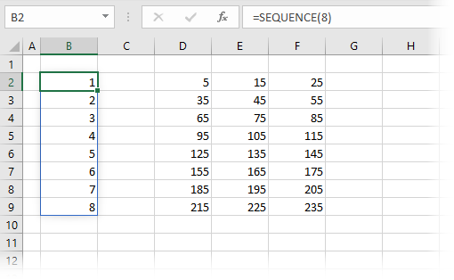
The formula in cell B2 is:
=SEQUENCE(8)In this formula, only the Rows argument is provided; all the other arguments ([Columns] optional, [Start] optional, and [Step] optional), have been excluded. Therefore, the default values are applied for each of these. SEQUENCE has created a list of sequential numbers; 8 rows, 1 column, starting at 1 and incrementing by 1 for each cell.
Including all arguments
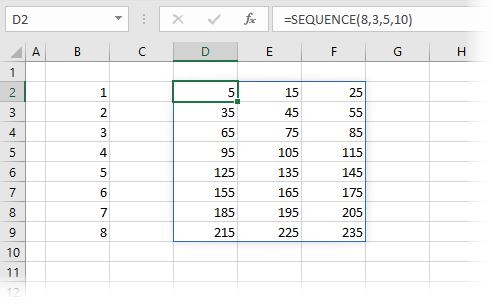
The formula in cell D2 uses all the arguments: Rows, Columns, Start and Step.
=SEQUENCE(8,3,5,10)When using the rows and columns arguments, it creates sequential numbers in a two-dimensional array. The formula is creating an array with:
- Rows argument = 8
- Columns argument = 3
- Start argument = 5
- Step argument = 10
The order of the numbers is important here, the function increments across the columns before moving to the next row.
Example 2 – Using SEQUENCE inside other functions
The example below shows how to use SEQUENCE inside the DATE function.
Note: As I am based in the UK, the screenshot below shows the UK date format (dd/mm/yyyy).
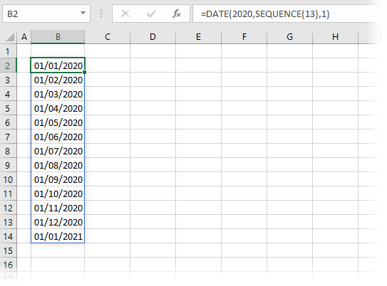
The formula in cell B2 is:
=DATE(2020,SEQUENCE(13),1)This formula creates a sequence of monthly dates starting on January 1st, 2020. The SEQUENCE function is applied to the month argument; therefore, it adds one to the month for each subsequent result. We have requested 13 months, but Excel is intelligent enough to know that 01/13/2020 doesn’t exist as a UK date format. Instead, the DATE function causes the result to roll-over into the next year and create 01/01/2021.
Example 3 – SEQUENCE row / column order
As already mentioned, the SEQUENCE formula in Excel creates sequential numbers across both rows and columns. However, by default they increment across columns before going down to the next row. To change this, we can use the TRANSPOSE function.
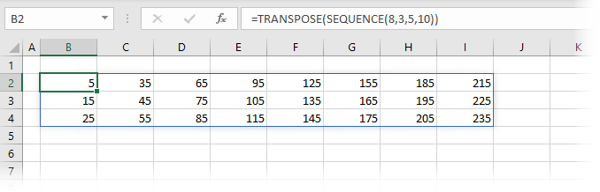
The formula in cell B2 is:
=TRANSPOSE(SEQUENCE(8,3,5,10))This is the same SEQUENCE function as we used in Example 1, but it has been wrapped in TRANSPOSE. Therefore, now the numbers increment down each row before going to the next column.
This can get a little confusing as while we have used the rows and columns arguments, the rows argument is displaying 8 columns and the column argument is displaying 3 rows. When we use this technique, we just need to remember that TRANSPOSE is applied as the last action.
Example 4 – Sequence with INDEX
The SEQUENCE formula in Excel is useful by itself, but when combined with other functions it’s power can be clearly seen.
In the screenshot below, we have a list of names and then the person’s ID or department. There are two rows for every individual. How can we get a list of just the ID’s sorted by last name? Let’s find out:
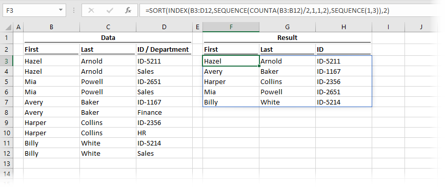
The formula in cell F2 is:
=SORT(INDEX(B3:D12,SEQUENCE(COUNTA(B3:B12)/2,1,1,2),SEQUENCE(1,3)),2)Let’s break this down:
- SEQUENCE(COUNTA(B3:B12)/2,1,1,2) – this part uses COUNTA to calculate the number of rows, then divides that by 2, as we want to return every 2nd row. SEQUENCE is then used to create the list which is 1 column, starts at the first row but steps by 2.
- SEQUENCE(1,3) – as we have 3 columns in our source, we want to return the same 3 columns. This creates the array list for INDEX to use.
- INDEX(B3:D12,…..) – The first SEQUENCE function above returns the value {1, 3, 5, 7, 9, 11}, the second SEQUENCE function above returns the values {1;2;3}. INDEX returns only the values from B3-B12 which are in these row and column positions.
- SORT(….,2) – finally the result is sorted by the 2nd column, which is the last name
This demonstrates the power of SEQUENCE as an enabler to more complex functions.
Example 5 – SEQUENCE in random order
Do you play bingo? No, me neither. But it creates an interesting example. I’m led to believe there are 75 numbers and those numbers can only appear once. By combining SORTBY, RANDARRAY and SEQUENCE we can put the sequence of 75 numbers into a random order (just like bingo).
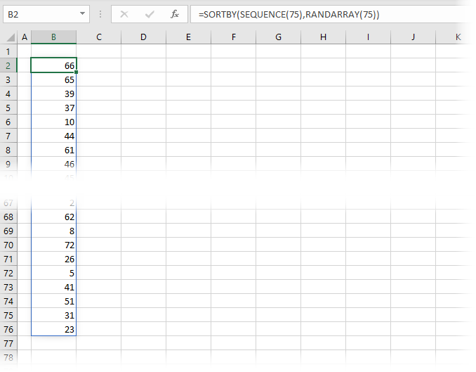
The formula in cell B2 is:
=SORTBY(SEQUENCE(75),RANDARRAY(75))The SEQUENCE function returns a list from 1 to 75. This list is sorted by another list of 75 random numbers created by RANDARRAY.
Other examples
The post about the SORT function also contains an example of using the SEQUENCE formula in Excel to create a list of the top 5 results.
Want to learn more?
There is a lot to learn about dynamic arrays and the new functions. Check out my other posts here to learn more:
- Introduction to dynamic arrays – learn how the excel calculation engine has changed.
- UNIQUE – to list the unique values in a range
- SORT – to sort the values in a range
- SORTBY – to sort values based on the order of other values
- FILTER – to return only the values which meet specific criteria
- SEQUENCE – to return a sequence of numbers in rows and columns
- RANDARRAY – to return an array of random numbers across a specific number of rows and columns
- Using dynamic arrays with other Excel features – learn to use dynamic arrays with charts, PivotTables, pictures etc
- Advanced dynamic array formula techniques – learn the advanced techniques for managing dynamic arrays

About the author
Hey, I’m Mark, and I run Excel Off The Grid.
My parents tell me that at the age of 7 I declared I was going to become a qualified accountant. I was either psychic or had no imagination, as that is exactly what happened. However, it wasn’t until I was 35 that my journey really began.
In 2015, I started a new job, for which I was regularly working after 10pm. As a result, I rarely saw my children during the week. So, I started searching for the secrets to automating Excel. I discovered that by building a small number of simple tools, I could combine them together in different ways to automate nearly all my regular tasks. This meant I could work less hours (and I got pay raises!). Today, I teach these techniques to other professionals in our training program so they too can spend less time at work (and more time with their children and doing the things they love).
Do you need help adapting this post to your needs?
I’m guessing the examples in this post don’t exactly match your situation. We all use Excel differently, so it’s impossible to write a post that will meet everybody’s needs. By taking the time to understand the techniques and principles in this post (and elsewhere on this site), you should be able to adapt it to your needs.
But, if you’re still struggling you should:
- Read other blogs, or watch YouTube videos on the same topic. You will benefit much more by discovering your own solutions.
- Ask the ‘Excel Ninja’ in your office. It’s amazing what things other people know.
- Ask a question in a forum like Mr Excel, or the Microsoft Answers Community. Remember, the people on these forums are generally giving their time for free. So take care to craft your question, make sure it’s clear and concise. List all the things you’ve tried, and provide screenshots, code segments and example workbooks.
- Use Excel Rescue, who are my consultancy partner. They help by providing solutions to smaller Excel problems.
What next?
Don’t go yet, there is plenty more to learn on Excel Off The Grid. Check out the latest posts:
Excel VBA Find Next
Like in Excel, when we press CTRL + F, a wizard box pops up, allowing us to search for a value in the given worksheet. Once we find the value, we click on “Find Next” to find the other similar value. As it is a worksheet feature, we can also use it in VBA as the Application property method as application.findnext for the same purposes.
Finding the specific value in the mentioned range is fine, but what if the requirement is to find the value with multiple occurrences? In one of the earlier articles, we discussed the “Find” method in VBA. It is not complex, but finding all the repetitive occurrences is possible only with the “FindNext” method in Excel VBA.
Table of contents
- Excel VBA Find Next
- What is Find Next in Excel VBA?
- Examples of Find Next Method in Excel VBA
- VBA Find Next (Using Loop)
- Things to Remember
- Recommended Articles
This article will show you how to use this “Find Next” in Excel VBA.
You are free to use this image on your website, templates, etc, Please provide us with an attribution linkArticle Link to be Hyperlinked
For eg:
Source: VBA Find Next (wallstreetmojo.com)
What is Find Next in Excel VBA?
As the word says, “Find Next” means from the found cell, keep searching for the next value until it returns to the original cell where we started the search.
The advanced version of the “Find” method searches only once the mentioned value is in the range.
Below is the syntax of the FINDNEXT method in Excel VBA.
![]()
After: It is the word that we are searching for.
Examples of Find Next Method in Excel VBA
Below are examples of finding the next method in Excel VBA.
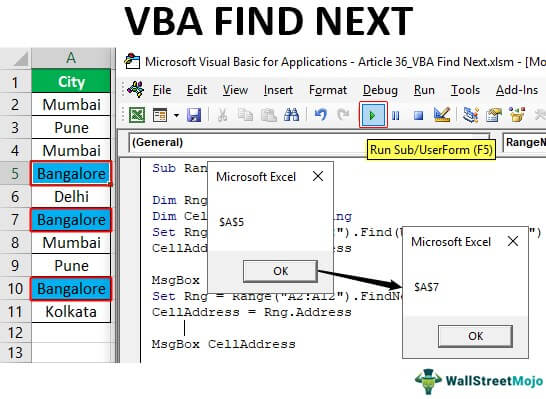
Look at the below data.
You can download this VBA Find Next Excel Template here – VBA Find Next Excel Template

Step #1 – In this data, we need to find the city name “Bangalore.” Let’s start the sub procedure in the visual basic editorThe Visual Basic for Applications Editor is a scripting interface. These scripts are primarily responsible for the creation and execution of macros in Microsoft software.read more.
Code:
Sub RangeNext_Example()

End Sub

Step #2 – First, declare the variable as a “Range” object.
Code:
Sub RangeNext_Example()

 Dim Rng As Range

End Sub

Step #3 – Set the reference for the object variable as “Range(“A2: A11”).
Code:
Sub RangeNext_Example()

 Dim Rng As Range
 Set Rng = Range("A2:A12")

End Sub

Since our data of the city list is in the range of cells from A2 to A11, only we will search for the city “Bangalore.”
Since we set the range reference to the variable “Rng,” we use this variable instead of using RANGE(“A2: A11”) every time.
Step #4 – Use the RNG variable and open the Find method.
Code:
Sub RangeNext_Example()

 Dim Rng As Range
 Set Rng = Range("A2:A12")
 Rng.Find

End Sub

Step #5 – The first argument of the FIND method is “What,” i.e., what we are trying to search in the mentioned range, so the value we are searching is “Bangalore.”
Code:
Sub RangeNext_Example()

 Dim Rng As Range
 Set Rng = Range("A2:A12")
 Rng.Find What:="Bangalore"

End Sub

Step #6 – To show which cell we found this value in, declare one more variable as a string.
Code:
Sub RangeNext_Example()

 Dim Rng As Range
 Dim CellAdderess As String

 Set Rng = Range("A2:A12")
 Rng.Find What:="Bangalore"

End Sub

Step #7 – For this variable, assign the found cell address.
Code:
Sub RangeNext_Example()

  Dim Rng As Range
  Dim CellAdderess As String

  Set Rng = Range("A2:A12").Find(What:="Bangalore")
  Rng.Find What:="Bangalore"

  CellAddress = Rng.Address

End Sub

Note: RNG. Address because RNG will have the reference for the found value cell.
Step #8 – Now show the assigned cell address variable result in the message box in VBA.
Sub RangeNext_Example()

 Dim Rng As Range
 Dim CellAdderess As String

 Set Rng = Range("A2:A12").Find(What:="Bangalore")
 Rng.Find What:="Bangalore"

 CellAddress = Rng.Address
 MsgBox CellAddress

End Sub

Step #9 – Run the code and see what we get here.

So we have found the value “Bangalore” in cell A5. However, we can find only one cell with the Find method, so instead of FIND, we need to use FINDNEXT in Excel VBA.
Step #10 – We need to reference the range object variable using the FINDNEXT method in Excel VBA.
Code:
Sub RangeNext_Example()

 Dim Rng As Range
 Dim CellAdderess As String
 Set Rng = Range("A2:A12").Find(What:="Bangalore")
 Rng.Find What:="Bangalore"

 CellAddress = Rng.Address
 MsgBox CellAddress

 Set Rng = Range("A2:A12").FindNext(Rng)

End Sub

As you can see above, we have used the VBA FINDNEXT method, but inside the function, we have used a range object variable name.
Step #11 – Now again, assign the cell address and show the address in the message box.
Code:
Sub RangeNext_Example()

 Dim Rng As Range
 Dim CellAdderess As String
 Set Rng = Range("A2:A12").Find(What:="Bangalore")
 Rng.Find What:="Bangalore"

 CellAddress = Rng.Address
 MsgBox CellAddress

 Set Rng = Range("A2:A12").FindNext(Rng)
 CellAddress = Rng.Address
 MsgBox CellAddress

End Sub

Step #12 – Run the macro and see what we get in the first message box.

Step #13 – The first message box shows the value “Bangalore” found in cell A5. Click on the “OK” button to see the next found value.

The second value found is in the A7 cell. Press “OK” to continue.
VBA Find Next (Using Loop)
It will exit the VBA subprocedureSUB in VBA is a procedure which contains all the code which automatically gives the statement of end sub and the middle portion is used for coding. Sub statement can be both public and private and the name of the subprocedure is mandatory in VBA.read more, but we are one more to be found in cell A10. When we find the values in more than one cell, it is better to use loops.
In this case, too, we have value “Bangalore” in more than one cell, so we need to include loops here.
Step #14 – First, declare two variables as the range.
Code:
Sub RangeNext_Example1()

 Dim Rng As Range
 Dim FindRng As Range

End Sub

Step #15 – Set the reference for the first variable, as shown below.
Code:
Sub RangeNext_Example1()

 Dim Rng As Range
 Dim FindRng As Range

 Set Rng = Range("A2:A11").Find(What:="Bangalore")

End Sub

Step #16 – Set the reference using the FIND VBA functionVBA Find gives the exact match of the argument. It takes three arguments, one is what to find, where to find and where to look at. If any parameter is missing, it takes existing value as that parameter.read more for the second variable.
Sub RangeNext_Example1()

 Dim Rng As Range
 Dim FindRng As Range

 Set Rng = Range("A2:A11").Find(What:="Bangalore")
 Set FindRng = Rng.FindNext("Bangalore")

End Sub

Step #17 – Before we start searching for the value, we need to identify from which cell we start the search, which declares the variable as a string.
Code:
Sub RangeNext_Example1()

 Dim Rng As Range
 Dim FindRng As Range

 Set Rng = Range("A2:A11").Find(What:="Bangalore")
 Set FindRng = Rng.FindNext("Bangalore")

 Dim FirstCell As String
 FirstCell = Rng.Address

End Sub

Step #18 – For this variable, assign the first cell address.
Code:
Sub RangeNext_Example1()

 Dim Rng As Range
 Dim FindRng As Range

 Set Rng = Range("A2:A11")
 Set FindRng = Rng.Find(What:="Bangalore")

 Dim FirstCell As String
 FirstCell = Rng.Address

End Sub

Step #19 – We need to include the “Do While” loop to loop through all the cells and find the searching value.
Code:
Sub RangeNext_Example1()

 Dim Rng As Range
 Dim FindRng As Range

 Set Rng = Range("A2:A11").Find(What:="Bangalore")
 Set FindRng = Rng.FindNext("Bangalore")

 Dim FirstCell As String
 FirstCell = Rng.Address

 Do
 Loop While FirstCell <> Cell.Address

End Sub

Inside the loop, mention the message box and VBA FINDNEXT method.
Step #20 – Below is the complete code for you.
Code:
Sub FindNext_Example()

 Dim FindValue As String
 FindValue = "Bangalore"

 Dim Rng As Range
 Set Rng = Range("A2:A11")

 Dim FindRng As Range
 Set FindRng = Rng.Find(What:=FindValue)

 Dim FirstCell As String
 FirstCell = FindRng.Address

 Do
  MsgBox FindRng.Address
  Set FindRng = Rng.FindNext(FindRng)
  Loop While FirstCell <> FindRng.Address

 MsgBox "Search is over"

End Sub
Step #21 – This will keep showing all the matching cell addresses, and in the end, it will show the message “Search is Over” in the new message box.

Things to Remember
- The FIND method can find only one value at a time.
- The FINDNEXT method in Excel VBA can find the next value from the already found value cell.
- We must use the Do While loop to loop through all the cells in the range.
Recommended Articles
This article has been a guide to VBA FINDNEXT. Here, we discuss how to find the specific value using Excel VBA FindNext function, along with examples. You can learn more about VBA functions from the following articles: –
- For Next Loop in VBA
- VBA ListObjects
- CDEC in VBA
- VBA Login User Form
Содержание
- Процедура вставки текста около формулы
- Способ 1: использование амперсанда
- Способ 2: применение функции СЦЕПИТЬ
- Вопросы и ответы
Довольно часто при работе в Excel существует необходимость рядом с результатом вычисления формулы вставить поясняющий текст, который облегчает понимание этих данных. Конечно, можно выделить для пояснений отдельный столбец, но не во всех случаях добавление дополнительных элементов является рациональным. Впрочем, в Экселе имеются способы поместить формулу и текст в одну ячейку вместе. Давайте разберемся, как это можно сделать при помощи различных вариантов.
Процедура вставки текста около формулы
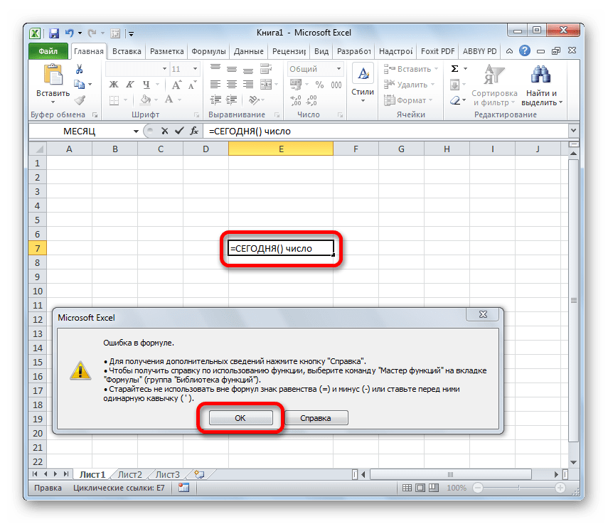
Если просто попробовать вставить текст в одну ячейку с функцией, то при такой попытке Excel выдаст сообщение об ошибке в формуле и не позволит совершить такую вставку. Но существует два способа все-таки вставить текст рядом с формульным выражением. Первый из них заключается в применении амперсанда, а второй – в использовании функции СЦЕПИТЬ.
Способ 1: использование амперсанда
Самый простой способ решить данную задачу – это применить символ амперсанда (&). Данный знак производит логическое отделение данных, которые содержит формула, от текстового выражения. Давайте посмотрим, как можно применить указанный способ на практике.
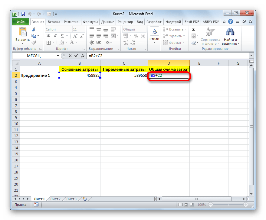
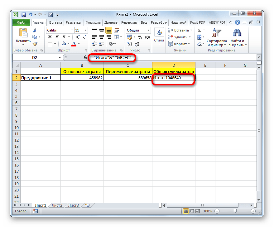
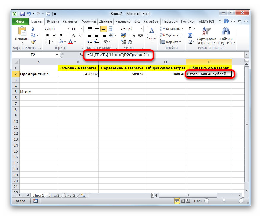
У нас имеется небольшая таблица, в которой в двух столбцах указаны постоянные и переменные затраты предприятия. В третьем столбце находится простая формула сложения, которая суммирует их и выводит общим итогом. Нам требуется в ту же ячейку, где отображается общая сумма затрат добавить после формулы поясняющее слово «рублей».

- Активируем ячейку, содержащую формульное выражение. Для этого либо производим по ней двойной щелчок левой кнопкой мыши, либо выделяем и жмем на функциональную клавишу F2. Также можно просто выделить ячейку, а потом поместить курсор в строку формул.
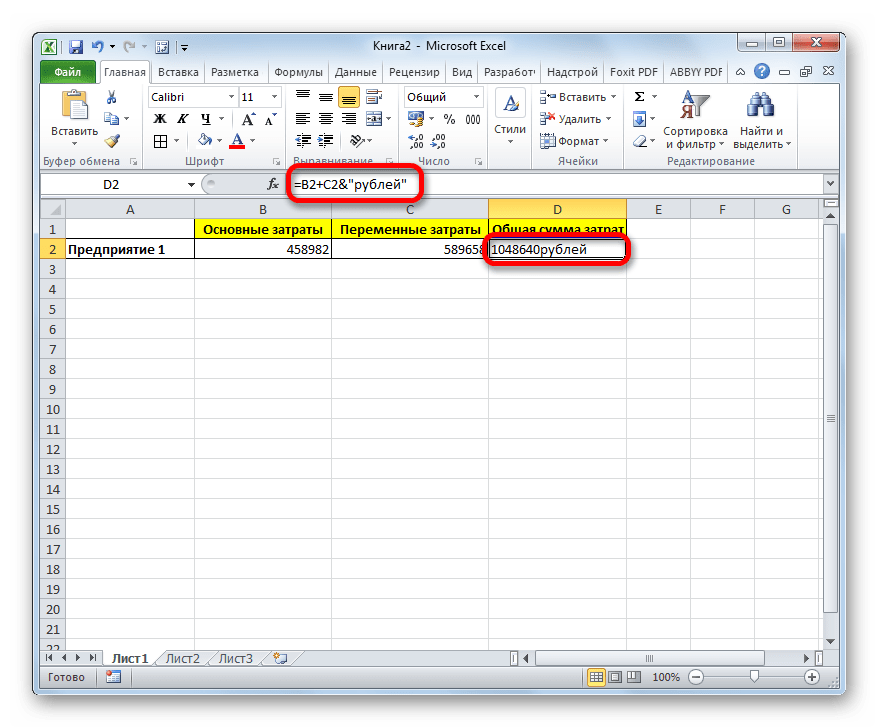
- Сразу после формулы ставим знак амперсанд (&). Далее в кавычках записываем слово «рублей». При этом кавычки не будут отображаться в ячейке после числа выводимого формулой. Они просто служат указателем для программы, что это текст. Для того, чтобы вывести результат в ячейку, щелкаем по кнопке Enter на клавиатуре.
- Как видим, после этого действия, вслед за числом, которое выводит формула, находится пояснительная надпись «рублей». Но у этого варианта есть один видимый недостаток: число и текстовое пояснение слились воедино без пробела.

При этом, если мы попытаемся поставить пробел вручную, то это ничего не даст. Как только будет нажата кнопка Enter, результат снова «склеится».
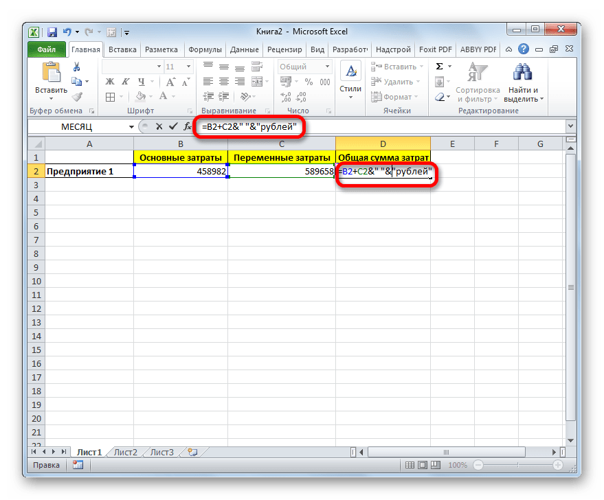
- Но из сложившейся ситуации все-таки существует выход. Снова активируем ячейку, которая содержит формульное и текстовое выражения. Сразу после амперсанда открываем кавычки, затем устанавливаем пробел, кликнув по соответствующей клавише на клавиатуре, и закрываем кавычки. После этого снова ставим знак амперсанда (&). Затем щелкаем по клавише Enter.
- Как видим, теперь результат вычисления формулы и текстовое выражение разделены пробелом.


Естественно, что все указанные действия проделывать не обязательно. Мы просто показали, что при обычном введении без второго амперсанда и кавычек с пробелом, формульные и текстовые данные сольются. Вы же можете установить правильный пробел ещё при выполнении второго пункта данного руководства.
При написании текста перед формулой придерживаемся следующего синтаксиса. Сразу после знака «=» открываем кавычки и записываем текст. После этого закрываем кавычки. Ставим знак амперсанда. Затем, в случае если нужно внести пробел, открываем кавычки, ставим пробел и закрываем кавычки. Щелкаем по клавише Enter.

Для записи текста вместе с функцией, а не с обычной формулой, все действия точно такие же, как были описаны выше.
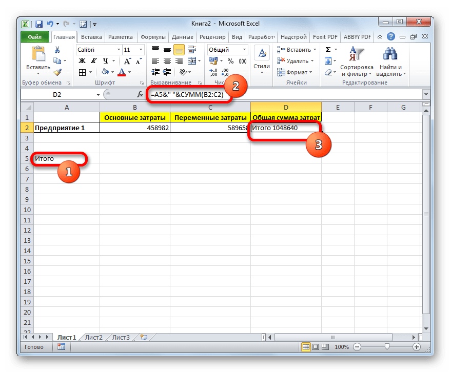
Текст также можно указывать в виде ссылки на ячейку, в которой он расположен. В этом случае, алгоритм действий остается прежним, только сами координаты ячейки в кавычки брать не нужно.
Способ 2: применение функции СЦЕПИТЬ
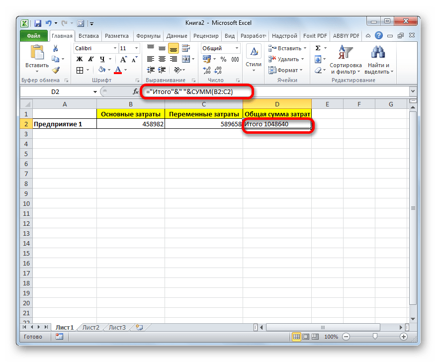
Также для вставки текста вместе с результатом подсчета формулы можно использовать функцию СЦЕПИТЬ. Данный оператор предназначен для того, чтобы соединять в одной ячейке значения, выводимые в нескольких элементах листа. Он относится к категории текстовых функций. Его синтаксис следующий:
=СЦЕПИТЬ(текст1;текст2;…)
Всего у этого оператора может быть от 1 до 255 аргументов. Каждый из них представляет либо текст (включая цифры и любые другие символы), либо ссылки на ячейки, которые его содержат.
Посмотрим, как работает данная функция на практике. Для примера возьмем все ту же таблицу, только добавим в неё ещё один столбец «Общая сумма затрат» с пустой ячейкой.
- Выделяем пустую ячейку столбца «Общая сумма затрат». Щелкаем по пиктограмме «Вставить функцию», расположенную слева от строки формул.
- Производится активация Мастера функций. Перемещаемся в категорию «Текстовые». Далее выделяем наименование «СЦЕПИТЬ» и жмем на кнопку «OK».
- Запускается окошко аргументов оператора СЦЕПИТЬ. Данное окно состоит из полей под наименованием «Текст». Их количество достигает 255, но для нашего примера понадобится всего три поля. В первом мы разместим текст, во втором – ссылку на ячейку, в которой содержится формула, и в третьем опять разместим текст.
Устанавливаем курсор в поле «Текст1». Вписываем туда слово «Итого». Писать текстовые выражения можно без кавычек, так как программа проставит их сама.
Потом переходим в поле «Текст2». Устанавливаем туда курсор. Нам нужно тут указать то значение, которое выводит формула, а значит, следует дать ссылку на ячейку, её содержащую. Это можно сделать, просто вписав адрес вручную, но лучше установить курсор в поле и кликнуть по ячейке, содержащей формулу на листе. Адрес отобразится в окошке аргументов автоматически.
В поле «Текст3» вписываем слово «рублей».
После этого щелкаем по кнопке «OK».
- Результат выведен в предварительно выделенную ячейку, но, как видим, как и в предыдущем способе, все значения записаны слитно без пробелов.
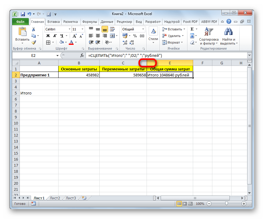
- Для того, чтобы решить данную проблему, снова выделяем ячейку, содержащую оператор СЦЕПИТЬ и переходим в строку формул. Там после каждого аргумента, то есть, после каждой точки с запятой добавляем следующее выражение:
" ";Между кавычками должен находиться пробел. В целом в строке функций должно отобразиться следующее выражение:
=СЦЕПИТЬ("Итого";" ";D2;" ";"рублей")Щелкаем по клавише ENTER. Теперь наши значения разделены пробелами.
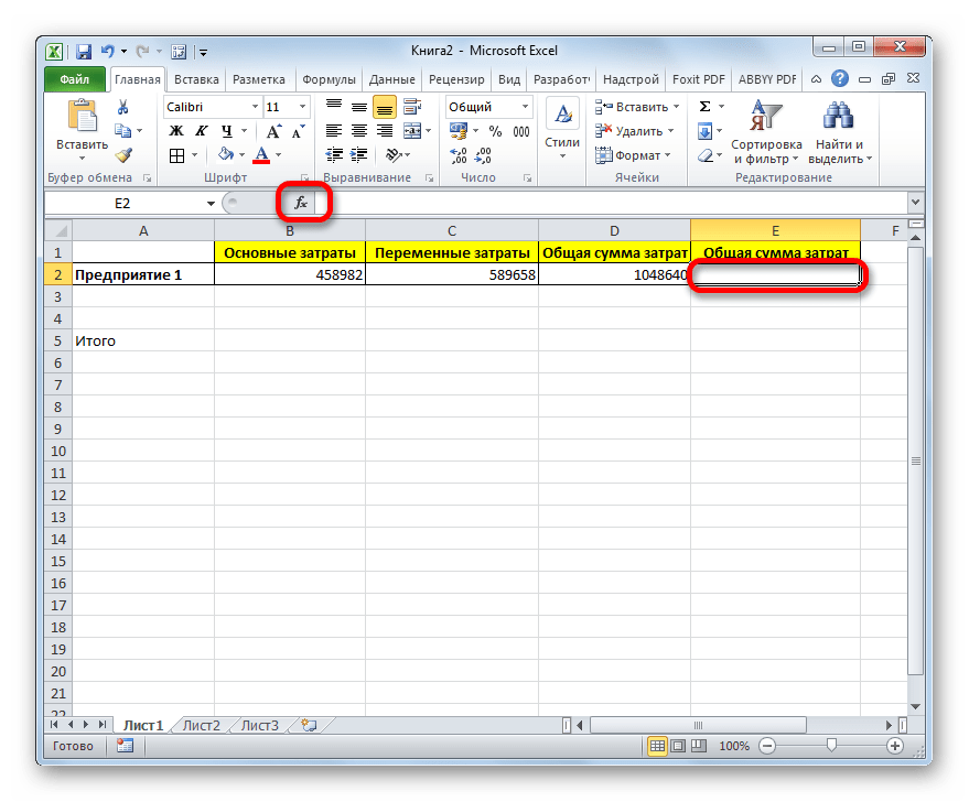
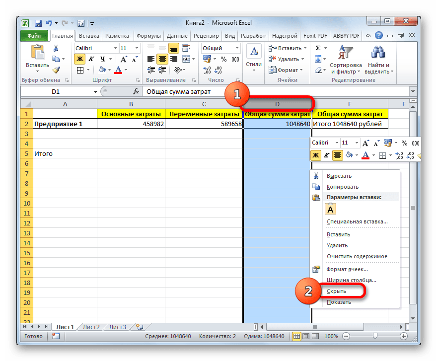
- При желании можно спрятать первый столбец «Общая сумма затрат» с исходной формулой, чтобы он не занимал лишнее место на листе. Просто удалить его не получится, так как это нарушит функцию СЦЕПИТЬ, но убрать элемент вполне можно. Кликаем левой кнопкой мыши по сектору панели координат того столбца, который следует скрыть. После этого весь столбец выделяется. Щелкаем по выделению правой кнопкой мыши. Запускается контекстное меню. Выбираем в нем пункт «Скрыть».
- После этого, как видим, ненужный нам столбец скрыт, но при этом данные в ячейке, в которой расположена функция СЦЕПИТЬ отображаются корректно.


Читайте также: Функция СЦЕПИТЬ в Экселе
Как скрыть столбцы в Экселе
Таким образом, можно сказать, что существуют два способа вписать в одну ячейку формулу и текст: при помощи амперсанда и функции СЦЕПИТЬ. Первый вариант проще и для многих пользователей удобнее. Но, тем не менее, в определенных обстоятельствах, например при обработке сложных формул, лучше пользоваться оператором СЦЕПИТЬ.
There is no explicit Between formula in Excel, however, we can come up with creative ways to create this functionality. Our goal is to evaluate if a given value is between a range, for example, is 6 between 1 and 10?
We have three possible scenarios:
- Between formula in Excel for Numbers
- Between formula in Excel for Dates
- Between formula in Excel for Text
You can download this Excel Workbook and follow along:
DOWNLOAD EXCEL WORKBOOK
Between formula in Excel for Numbers
OPTION 1:Using a combination of MIN, MAX & AND function
In the example below, you have the start of the range in Column A, end of the range in Column B and the value to be evaluated in Column C.
You need to check whether the number entered in Column C is in between the numbers in Column A & Column B using a creatively formulated BETWEEN formula in Excel.

The function that can be used to determine if the value in cell D7 is in-between values in cell A7 & B7 is
=IF(AND(C7>=MIN(A7,B7),C7<=MAX(A7,B7)), “Yes”, “No”)
Let’s break this formula into parts to understand it better:
- C7 >= MIN(A7, B7) – This expression checks whether the value in cell C7 is greater than (or equal to) the smaller of the two numbers in cell A7 and B7.
- C7 <= MAX(A7, B7) – This expression checks whether the value in cell C7 is smaller than (or equal to) the larger of the two numbers in cell A7 and B7.
- AND( C7 >= MIN(A7, B7), C7 <= MAX(A7, B7)) – AND function simply checks whether the above two conditions are met or not i.e. whether the value in cell C7 is greater than (or equal to) the smaller number and less than (or equal to) the larger number.

OPTION 2:Using a MEDIAN function
You can use a simpler version of this complicated function by creatively using the Median formula:

=IF(C7=MEDIAN(A7:C7), “Yes”, “No”)
In our first example above, the range is 20-60, upon checking the value 50, it is in between this range.
The median formula will return the value in the middle of these 3 values when arranged in increasing order: 20, 50, 60. The median value is 50.
Since it matches the value we are evaluating, then the answer we get is a Yes, this value (50) is in between the range.
Now that you have learned how to use Excel if between two numbers, let’s move forward to dates and text.
Between formula in Excel for Dates
Irrespective of how you format a cell to display a date, Excel always stores it as a number. The number stored for each date actually represents the number of days since 0-Jan-1990.
1st Jan 1990 is stored as 1 (representing 1 day since 0-Jan-1990) and 23rd June 2020 is stored as 44,005 (representing 44005 days since 0-Jan-1990).
So, to check whether a date is in between two mentioned dates, we have the same application as the median formula.
Below is an example of how to use the median function to check dates.

=IF(C10=MEDIAN(A10:C10), “Yes”, “No”)
In our first example above, the range is May 1 – July 1, upon checking the date June 1, it is in between this range.
The median formula will return the value in the middle of these 3 dates when arranged in increasing order: May 1, June 1, July 1. The median value is June 1.
Since it matches the value we are evaluating, then the answer we get is a Yes, this value (June 1) is in between the range.
Between formula in Excel for Text
For text, we are checking if the value is alphabetically in the middle. We will be using the and formula:

=IF(AND(C12>=A12, C12<=B12, “Yes”, “No”)
Interestingly enough, you can compare texts using the >= and <= operators. Excel is able to compare them which goes alphabetically first or last.
In our first example above, the range is Cat – Dog, upon checking the text Cow, it is in between this range. As when arranged alphabetically, it would be: Cat, Cow, Dog.
The And formula checks if Cow >= Cat, and Cow <= Dog. You will see that both of these are true, as Cow is alphabetically later than Cat, while Cow is alphabetically ahead of Dog. Which is why we get a Yes result.
Conclusion
In this tutorial, you have learned how to use Between formula in Excel even when there is no explicit formula available to do this. You can use a combination of various other available function to create Excel if between range functionality.
You can use MIN, MAX, MEDIAN & AND functions to create a creative Between function in Excel for numbers, dates and text.
HELPFUL RESOURCE:

Make sure to download our FREE PDF on the 333 Excel keyboard Shortcuts here:


Цикл For Loop в VBA – один из самых популярных циклов в Excel. Данный цикл имеет две формы – For Next и For Each In Next. Данные операторы используются для последовательного перемещения по списку элементов или чисел. Для завершения цикла мы можем в любой момент использовать команду выхода. Давайте подробнее рассмотрим каждый из этих циклов.
Цикл For Next имеет следующий синтаксис:
|
1 |
For счетчик = начало_счетчика To конец_счетчика |
То что мы делаем здесь, по существу, это создаем цикл, который использует переменную счетчик как хранитель времени. Устанавливаем его значение равным начало_счетчика, и увеличиваем (или уменьшаем) на 1 во время каждого витка. Цикл будет выполняться до тех пор, пока значение счетчик не станет равным конец_счетчика. Когда оба эти значения совпадут, цикл выполнится последний раз и остановится.
Пример цикла
|
1 |
Sub пример_цикла1() |
Последнее значение переменной счетчик будет равным 11
VBA обратный цикл For Loop с инструкцией STEP
Если у вас появилась необходимость перемещаться от большего значения к меньшему – вы можете использовать цикл в обратном направлении. Вот пример обратного цикла:
|
1 |
Sub пример_цикла2() |
Последнее значение переменной счетчик будет равным 1.
Как вы могли заметить, мы можем использовать инструкцию Step n для работы цикла как вперед, так и в обратном направлении. По умолчанию значение Step равно 1, но оно может быть изменено, если необходимо пропускать какие-либо значения, тогда значение n будет больше одного, или перемещаться в обратном направлении, тогда n будет отрицательным.
VBA цикл For Each … Next
Цикл For Each … Next имеет следующий цикл:
|
1 |
For Each элемент_группы In группа_элементов |
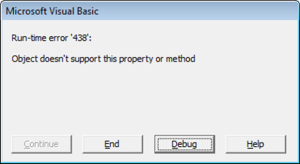
Здесь переменная элемент_группы принадлежит к группе_элементов (железная логика!!!). Я имею в виду, что объект группа_элементов должен быть коллекцией объектов. Вы не сможете запустить цикл For Each для отдельно объекта (Microsoft сразу оповестит вас об этом 438-й ошибкой).
Данный цикл перебирает все элементы какой-либо коллекции, начиная с самого первого. Вы можете использовать данный цикл, если вам необходимо, например, обойти все листы в книге, объекты на листе, сводные таблицы и т.д.
Ниже представлен пример, как можно воспользоваться циклом For Each для просмотра всех листов книги:
|
1 |
Sub пример_цикла4() |
… либо всех сводных таблиц на листе
|
1 |
Sub пример_цикла() |
Прерывание цикла VBA
Если вам необходимо выйти из цикла до момента, как будет достигнуто условие завершения цикла, воспользуйтесь командой End For в связке с инструкцией IF. В примере, приведенном ниже, мы выйдем из цикла до момента достижения условия завершения, в данном цикле выход будет осуществлен при условии, когда переменная счетчик будет равна 3.
|
1 |
Sub пример_цикла5() |
Пропуск части цикла в For Each
Пропускать часть цикла, а затем возвращаться назад – плохая практика. Тем не менее, давайте рассмотрим пример:
|
1 |
Sub пример_цикла6 () |
Здесь мы пропустили одну итерацию (когда j = 3). Как вы думаете, какой результат выдаст программа? 3? 5? Ну… на самом деле, ни один из вариантов не верный. Цикл будет выполняться бесконечно, пока память компьютера не переполнится.
Однако возможность пропустить шаг цикла без последствий существует. Вы можете увеличить значение счетчика на 1 (или другое значение), что приведет к пропуску операций, находящихся между этими значениями. Вот пример:
|
1 |
Sub пример_цикла7() |
Но опять же, это плохая практика написания кода, и может привести к нежелательным последствиям при написании кода в будущем. Вместо этого, при необходимости пропуска некоторых итераций, попробуйте использовать функцию If или Select Case.