
Содержание
- Looping Through a Range of Cells
- Support and feedback
- Excel VBA Ranges and Cells
- Ranges and Cells in VBA
- Cell Address
- A1 Notation
- R1C1 Notation
- Range of Cells
- A1 Notation
- R1C1 Notation
- Writing to Cells
- Reading from Cells
- Non Contiguous Cells
- VBA Coding Made Easy
- Intersection of Cells
- Offset from a Cell or Range
- Offset Syntax
- Offset from a cell
- Offset from a Range
- Setting Reference to a Range
- Resize a Range
- Resize Syntax
- OFFSET vs Resize
- All Cells in Sheet
- UsedRange
- CurrentRegion
- Range Properties
- Last Cell in Sheet
- Last Used Row Number in a Column
- Last Used Column Number in a Row
- Cell Properties
- Common Properties
- Cell Font
- Copy and Paste
- Paste All
- Paste Special
- AutoFit Contents
- More Range Examples
- For Each
- Range Address
- Range to Array
- Array to Range
- Sum Range
- Count Range
- VBA Code Examples Add-in
- Range.FindNext method (Excel)
- Syntax
- Parameters
- Return value
- Remarks
- Example
- Support and feedback
- Проход по диапазону ячеек
- Поддержка и обратная связь
- Jump to the Next Data Entry Cell in Excel
- Select the Data Entry Cells
- Name the Range
- Use the Named Range for Data Entry
- Video: Jump to the Next Data Entry Cell
- 0 thoughts on “Jump to the Next Data Entry Cell in Excel”
Looping Through a Range of Cells
When using Visual Basic, you often need to run the same block of statements on each cell in a range of cells. To do this, you combine a looping statement and one or more methods to identify each cell, one at a time, and run the operation.
One way to loop through a range is to use the For. Next loop with the Cells property. Using the Cells property, you can substitute the loop counter (or other variables or expressions) for the cell index numbers. In the following example, the variable counter is substituted for the row index. The procedure loops through the range C1:C20, setting to 0 (zero) any number whose absolute value is less than 0.01.
Another easy way to loop through a range is to use a For Each. Next loop with the collection of cells specified in the Range property. Visual Basic automatically sets an object variable for the next cell each time the loop runs. The following procedure loops through the range A1:D10, setting to 0 (zero) any number whose absolute value is less than 0.01.
If you don’t know the boundaries of the range you want to loop through, you can use the CurrentRegion property to return the range that surrounds the active cell. For example, the following procedure, when run from a worksheet, loops through the range that surrounds the active cell, setting to 0 (zero) any number whose absolute value is less than 0.01.
Support and feedback
Have questions or feedback about Office VBA or this documentation? Please see Office VBA support and feedback for guidance about the ways you can receive support and provide feedback.
Источник
Excel VBA Ranges and Cells
In this Article
Ranges and Cells in VBA
Excel spreadsheets store data in Cells. Cells are arranged into Rows and Columns. Each cell can be identified by the intersection point of it’s row and column (Exs. B3 or R3C2).
An Excel Range refers to one or more cells (ex. A3:B4)
Cell Address
A1 Notation
In A1 notation, a cell is referred to by it’s column letter (from A to XFD) followed by it’s row number(from 1 to 1,048,576). This is called a cell address.
In VBA you can refer to any cell using the Range Object.
R1C1 Notation
In R1C1 Notation a cell is referred by R followed by Row Number then letter ‘C’ followed by the Column Number. eg B4 in R1C1 notation will be referred by R4C2. In VBA you use the Cells Object to use R1C1 notation:
Range of Cells
A1 Notation
To refer to a more than one cell use a “:” between the starting cell address and last cell address. The following will refer to all the cells from A1 to D10:
R1C1 Notation
To refer to a more than one cell use a “,” between the starting cell address and last cell address. The following will refer to all the cells from A1 to D10:
Writing to Cells
To write values to a cell or contiguous group of cells, simple refer to the range, put an = sign and then write the value to be stored:
Reading from Cells
To read values from cells, simple refer to the variable to store the values, put an = sign and then refer to the range to be read:
Note: To store values from a range of cells, you need to use an Array instead of a simple variable.
Non Contiguous Cells
To refer to non contiguous cells use a comma between the cell addresses:
VBA Coding Made Easy
Stop searching for VBA code online. Learn more about AutoMacro — A VBA Code Builder that allows beginners to code procedures from scratch with minimal coding knowledge and with many time-saving features for all users!

Intersection of Cells
To refer to non contiguous cells use a space between the cell addresses:
Offset from a Cell or Range
Using the Offset function, you can move the reference from a given Range (cell or group of cells) by the specified number_of_rows, and number_of_columns.
Offset Syntax
Offset from a cell
Offset from a Range
Setting Reference to a Range
To assign a range to a range variable: declare a variable of type Range then use the Set command to set it to a range. Please note that you must use the SET command as RANGE is an object:
Resize a Range
Resize method of Range object changes the dimension of the reference range:
Top-left cell of the Resized range is same as the top-left cell of the original range
Resize Syntax
OFFSET vs Resize
Offset does not change the dimensions of the range but moves it by the specified number of rows and columns. Resize does not change the position of the original range but changes the dimensions to the specified number of rows and columns.
All Cells in Sheet
The Cells object refers to all the cells in the sheet (1048576 rows and 16384 columns).
UsedRange
UsedRange property gives you the rectangular range from the top-left cell used cell to the right-bottom used cell of the active sheet.
CurrentRegion
CurrentRegion property gives you the contiguous rectangular range from the top-left cell to the right-bottom used cell containing the referenced cell/range.
Range Properties
You can get Address, row/column number of a cell, and number of rows/columns in a range as given below:
Last Cell in Sheet
You can use Rows.Count and Columns.Count properties with Cells object to get the last cell on the sheet:
Last Used Row Number in a Column
END property takes you the last cell in the range, and End(xlUp) takes you up to the first used cell from that cell.
Last Used Column Number in a Row
END property takes you the last cell in the range, and End(xlToLeft) takes you left to the first used cell from that cell.
You can also use xlDown and xlToRight properties to navigate to the first bottom or right used cells of the current cell.
Cell Properties
Common Properties
Here is code to display commonly used Cell Properties
Cell Font
Cell.Font object contains properties of the Cell Font:
Copy and Paste
Paste All
Ranges/Cells can be copied and pasted from one location to another. The following code copies all the properties of source range to destination range (equivalent to CTRL-C and CTRL-V)
Paste Special
Selected properties of the source range can be copied to the destination by using PASTESPECIAL option:
Here are the possible options for the Paste option:
AutoFit Contents
Size of rows and columns can be changed to fit the contents using AutoFit:
More Range Examples
It is recommended that you use Macro Recorder while performing the required action through the GUI. It will help you understand the various options available and how to use them.
For Each
It is easy to loop through a range using For Each construct as show below:
At each iteration of the loop one cell in the range is assigned to the variable cell and statements in the For loop are executed for that cell. Loop exits when all the cells are processed.
Sort is a method of Range object. You can sort a range by specifying options for sorting to Range.Sort. The code below will sort the columns A:C based on key in cell C2. Sort Order can be xlAscending or xlDescending. Header:= xlYes should be used if first row is the header row.
Find is also a method of Range Object. It find the first cell having content matching the search criteria and returns the cell as a Range object. It return Nothing if there is no match.
Use FindNext method (or FindPrevious) to find next(previous) occurrence.
Following code will change the font to “Arial Black” for all cells in the range which start with “John”:
Following code will replace all occurrences of “To Test” to “Passed” in the range specified:
It is important to note that you must specify a range to use FindNext. Also you must provide a stopping condition otherwise the loop will execute forever. Normally address of the first cell which is found is stored in a variable and loop is stopped when you reach that cell again. You must also check for the case when nothing is found to stop the loop.
Range Address
Use Range.Address to get the address in A1 Style
Use xlReferenceStyle (default is xlA1) to get addres in R1C1 style
This is useful when you deal with ranges stored in variables and want to process for certain addresses only.
Range to Array
It is faster and easier to transfer a range to an array and then process the values. You should declare the array as Variant to avoid calculating the size required to populate the range in the array. Array’s dimensions are set to match number of values in the range.
Array to Range
After processing you can write the Array back to a Range. To write the Array in the example above to a Range you must specify a Range whose size matches the number of elements in the Array.
Use the code below to write the Array to the range D1:D5:
Please note that you must Transpose the Array if you write it to a row.
Sum Range
You can use many functions available in Excel in your VBA code by specifying Application.WorkSheetFunction. before the Function Name as in the example above.
Count Range
Written by: Vinamra Chandra

VBA Code Examples Add-in
Easily access all of the code examples found on our site.
Simply navigate to the menu, click, and the code will be inserted directly into your module. .xlam add-in.
Источник
Range.FindNext method (Excel)
Continues a search that was begun with the Find method. Finds the next cell that matches those same conditions and returns a Range object that represents that cell. This does not affect the selection or the active cell.
Syntax
expression.FindNext (After)
expression A variable that represents a Range object.
Parameters
| Name | Required/Optional | Data type | Description |
|---|---|---|---|
| After | Optional | Variant | The cell after which you want to search. This corresponds to the position of the active cell when a search is done from the user interface. Be aware that After must be a single cell in the range. |
| Remember that the search begins after this cell; the specified cell is not searched until the method wraps back around to this cell. If this argument is not specified, the search starts after the cell in the upper-left corner of the range. |
Return value
When the search reaches the end of the specified search range, it wraps around to the beginning of the range. To stop a search when this wraparound occurs, save the address of the first found cell, and then test each successive found-cell address against this saved address.
Example
This example finds all cells in the range A1:A500 on worksheet one that contain the value 2, and changes the entire cell value to 5. That is, the values 1234 and 99299 both contain 2 and both cell values will become 5.
This example finds all the cells in the first four columns that contain a constant X, and hides the column that contains the X.
This example finds all the cells in the first four columns that contain a constant X, and unhides the column that contains the X.
Support and feedback
Have questions or feedback about Office VBA or this documentation? Please see Office VBA support and feedback for guidance about the ways you can receive support and provide feedback.
Источник
Проход по диапазону ячеек
При использовании Visual Basic часто требуется выполнить один и тот же блок операторов в каждой ячейке диапазона. Для этого необходимо объединить оператор цикла и один или несколько методов для идентификации каждой ячейки по отдельности и выполнить операцию.
Один из способов пройти по диапазону — использовать цикл For. Next со свойством Cells. С помощью свойства Cells можно заменить номера индексов ячеек счетчиком циклов (или другими переменными или выражениями). В следующем примере индекс строки заменяется переменной counter . Процедура проходит по диапазону ячеек C1:C20, присваивая значение 0 (ноль) каждому числу, абсолютное значение которого меньше 0,01.
Еще один простой способ пройти по диапазону — использовать цикл For Each. Next с коллекцией ячеек, указанной в свойстве Range. Visual Basic автоматически присваивает объектную переменную для следующей ячейки при каждом выполнении цикла. Следующая процедура проходит по диапазону ячеек A1:D10, присваивая значение 0 (ноль) каждому числу, абсолютное значение которого меньше 0,01.
Если вы не знаете границы диапазона, по которому нужно пройти, можно использовать свойство CurrentRegion, чтобы возвратить диапазон, окружающий активную ячейку. Например, при запуске на листе следующая процедура выполняет проход по диапазону, окружающему активную ячейку, присваивая значение 0 (ноль) каждому числу, абсолютное значение которого меньше 0,01.
Поддержка и обратная связь
Есть вопросы или отзывы, касающиеся Office VBA или этой статьи? Руководство по другим способам получения поддержки и отправки отзывов см. в статье Поддержка Office VBA и обратная связь.
Источник
Jump to the Next Data Entry Cell in Excel
If you’re filling in a form, the data entry cells might be scattered throughout the worksheet. You’d like a quick and easy way to move through the cells, in a specific order. Here is a technique that lets you jump to the next data entry cell in Excel, without any macros.
Select the Data Entry Cells
To set up this technique, you will create a named range. The steps below show how to do this.
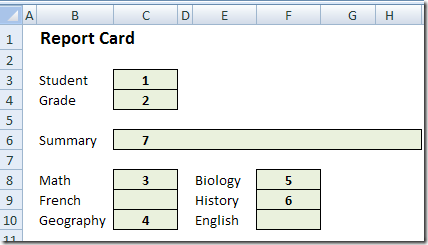
In this example, we have a report card, and the cells are numbered, to show the data entry order.
- First, select the second cell in which you want to enter data.
- In this example, we’ll select cell C4, where the student’s grade level will be entered.
- Then, hold the Ctrl key and select the next cell, then the next, until the remaining cells, 3 to 7, are selected.
- Finally, select the first cell in the sequence – cell C3 in this example.
Because cell C3 was selected last, it becomes the active cell in the range. Later, when we use this range, we’ll automatically start in cell C3.
- Note: In Excel 2003 and earlier versions, you’re limited to 255 characters in the named range formula. Depending on the length of the sheet name, you’ll probably be able to include 10-15 cells in the named range.
Name the Range
Next, you’ll create a name for the selected cells.
- Click in the Name box
- Type a one-word name for this group of cells – Grades in this example.
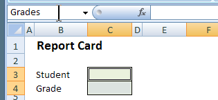
- Press the Enter key to save this name.
Use the Named Range for Data Entry
Now, when you want to enter information into these cells, you can select the named range, and tab through the cells.
- At the right of the Name box, click the drop-down arrow.
- Click on the name that you created – Grades
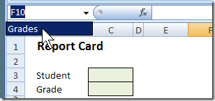
- With the named range selected, type in the active cell.
- Press the Tab key, or the Enter key, to move to the next cell.
- When all the cells are completed, click a cell outside the named range, to deselect the range.
Video: Jump to the Next Data Entry Cell
To see the technique to jump to the next data entry cell in Excel, watch this short video.
For more data entry tips and video, go to the Excel Data Entry Tips page on my Contextures website.
0 thoughts on “Jump to the Next Data Entry Cell in Excel”
This may sound surprising, but the 255 character limit does not apply here, provided you use the name box to define the name after selecting the data entry cells.
The actual limit is a certain amount of areas (I forgot how many).
The only way to EDIT that name afterwards however is by using Name Manager created by Charles Williams and myself, download at
http://www.jkp-ads.com/officemarketplacenm-en.asp
@ JKP
Name manager is not the only way to edit the name. In XL 2003 I just used Insert – Name – Define to manually add another cell to the range. You can edit the content of the “Refers to:” box and click “Add” to make changes. If you hit F2 while in the “Refers to:” box, you can use the arrow keys to navigate and enter new cell addresses.
Well I never – after all the years I have been using Excel I have never used this technique – Many thanks for sharing it with us.
Lots of my customers will find this very useful and I will be passing it on with a reference to your excellent blog.
Thanks Clayton — glad you found the tip useful!
Источник
На чтение 18 мин. Просмотров 75k.

сэр Артур Конан Дойл
Это большая ошибка — теоретизировать, прежде чем кто-то получит данные
Эта статья охватывает все, что вам нужно знать об использовании ячеек и диапазонов в VBA. Вы можете прочитать его от начала до конца, так как он сложен в логическом порядке. Или использовать оглавление ниже, чтобы перейти к разделу по вашему выбору.
Рассматриваемые темы включают свойство смещения, чтение
значений между ячейками, чтение значений в массивы и форматирование ячеек.
Содержание
- Краткое руководство по диапазонам и клеткам
- Введение
- Важное замечание
- Свойство Range
- Свойство Cells рабочего листа
- Использование Cells и Range вместе
- Свойство Offset диапазона
- Использование диапазона CurrentRegion
- Использование Rows и Columns в качестве Ranges
- Использование Range вместо Worksheet
- Чтение значений из одной ячейки в другую
- Использование метода Range.Resize
- Чтение Value в переменные
- Как копировать и вставлять ячейки
- Чтение диапазона ячеек в массив
- Пройти через все клетки в диапазоне
- Форматирование ячеек
- Основные моменты
Краткое руководство по диапазонам и клеткам
| Функция | Принимает | Возвращает | Пример | Вид |
| Range | адреса ячеек |
диапазон ячеек |
.Range(«A1:A4») | $A$1:$A$4 |
| Cells | строка, столбец |
одна ячейка |
.Cells(1,5) | $E$1 |
| Offset | строка, столбец |
диапазон | .Range(«A1:A2») .Offset(1,2) |
$C$2:$C$3 |
| Rows | строка (-и) | одна или несколько строк |
.Rows(4) .Rows(«2:4») |
$4:$4 $2:$4 |
| Columns | столбец (-цы) |
один или несколько столбцов |
.Columns(4) .Columns(«B:D») |
$D:$D $B:$D |
Введение
Это третья статья, посвященная трем основным элементам VBA. Этими тремя элементами являются Workbooks, Worksheets и Ranges/Cells. Cells, безусловно, самая важная часть Excel. Почти все, что вы делаете в Excel, начинается и заканчивается ячейками.
Вы делаете три основных вещи с помощью ячеек:
- Читаете из ячейки.
- Пишите в ячейку.
- Изменяете формат ячейки.
В Excel есть несколько методов для доступа к ячейкам, таких как Range, Cells и Offset. Можно запутаться, так как эти функции делают похожие операции.
В этой статье я расскажу о каждом из них, объясню, почему они вам нужны, и когда вам следует их использовать.
Давайте начнем с самого простого метода доступа к ячейкам — с помощью свойства Range рабочего листа.
Важное замечание
Я недавно обновил эту статью, сейчас использую Value2.
Вам может быть интересно, в чем разница между Value, Value2 и значением по умолчанию:
' Value2
Range("A1").Value2 = 56

' Value
Range("A1").Value = 56

' По умолчанию используется значение
Range("A1") = 56
Использование Value может усечь число, если ячейка отформатирована, как валюта. Если вы не используете какое-либо свойство, по умолчанию используется Value.
Лучше использовать Value2, поскольку он всегда будет возвращать фактическое значение ячейки.
Свойство Range
Рабочий лист имеет свойство Range, которое можно использовать для доступа к ячейкам в VBA. Свойство Range принимает тот же аргумент, что и большинство функций Excel Worksheet, например: «А1», «А3: С6» и т.д.
В следующем примере показано, как поместить значение в ячейку с помощью свойства Range.
Sub ZapisVYacheiku()

    ' Запишите число в ячейку A1 на листе 1 этой книги
    ThisWorkbook.Worksheets("Лист1").Range("A1").Value2 = 67

    ' Напишите текст в ячейку A2 на листе 1 этой рабочей книги
    ThisWorkbook.Worksheets("Лист1").Range("A2").Value2 = "Иван Петров"

    ' Запишите дату в ячейку A3 на листе 1 этой книги
    ThisWorkbook.Worksheets("Лист1").Range("A3").Value2 = #11/21/2019#

End Sub
Как видно из кода, Range является членом Worksheets, которая, в свою очередь, является членом Workbook. Иерархия такая же, как и в Excel, поэтому должно быть легко понять. Чтобы сделать что-то с Range, вы должны сначала указать рабочую книгу и рабочий лист, которому она принадлежит.
В оставшейся части этой статьи я буду использовать кодовое имя для ссылки на лист.

Следующий код показывает приведенный выше пример с использованием кодового имени рабочего листа, т.е. Лист1 вместо ThisWorkbook.Worksheets («Лист1»).
Sub IspKodImya ()

    ' Запишите число в ячейку A1 на листе 1 этой книги
     Sheet1.Range("A1").Value2 = 67

    ' Напишите текст в ячейку A2 на листе 1 этой рабочей книги
    Sheet1.Range("A2").Value2 = "Иван Петров"

    ' Запишите дату в ячейку A3 на листе 1 этой книги
    Sheet1.Range("A3").Value2 = #11/21/2019#

End Sub
Вы также можете писать в несколько ячеек, используя свойство
Range
Sub ZapisNeskol()

    ' Запишите число в диапазон ячеек
    Sheet1.Range("A1:A10").Value2 = 67

    ' Написать текст в несколько диапазонов ячеек
    Sheet1.Range("B2:B5,B7:B9").Value2 = "Иван Петров"

End Sub
Свойство Cells рабочего листа
У Объекта листа есть другое свойство, называемое Cells, которое очень похоже на Range . Есть два отличия:
- Cells возвращают диапазон только одной ячейки.
- Cells принимает строку и столбец в качестве аргументов.
В приведенном ниже примере показано, как записывать значения
в ячейки, используя свойства Range и Cells.
Sub IspCells()

    ' Написать в А1
    Sheet1.Range("A1").Value2 = 10
    Sheet1.Cells(1, 1).Value2  = 10

    ' Написать в А10
    Sheet1.Range("A10").Value2 = 10
    Sheet1.Cells(10, 1).Value2  = 10

    ' Написать в E1
    Sheet1.Range("E1").Value2 = 10
    Sheet1.Cells(1, 5).Value2  = 10

End Sub
Вам должно быть интересно, когда использовать Cells, а когда Range. Использование Range полезно для доступа к одним и тем же ячейкам при каждом запуске макроса.
Например, если вы использовали макрос для вычисления суммы и
каждый раз записывали ее в ячейку A10, тогда Range подойдет для этой задачи.
Использование свойства Cells полезно, если вы обращаетесь к
ячейке по номеру, который может отличаться. Проще объяснить это на примере.
В следующем коде мы просим пользователя указать номер столбца. Использование Cells дает нам возможность использовать переменное число для столбца.
Sub ZapisVPervuyuPustuyuYacheiku()

    Dim UserCol As Integer

    ' Получить номер столбца от пользователя
    UserCol = Application.InputBox("Пожалуйста, введите номер столбца...", Type:=1)

    ' Написать текст в выбранный пользователем столбец
    Sheet1.Cells(1, UserCol).Value2 = "Иван Петров"

End Sub
В приведенном выше примере мы используем номер для столбца,
а не букву.
Чтобы использовать Range здесь, потребуется преобразовать эти значения в ссылку на
буквенно-цифровую ячейку, например, «С1». Использование свойства Cells позволяет нам
предоставить строку и номер столбца для доступа к ячейке.
Иногда вам может понадобиться вернуть более одной ячейки, используя номера строк и столбцов. В следующем разделе показано, как это сделать.
Использование Cells и Range вместе
Как вы уже видели, вы можете получить доступ только к одной ячейке, используя свойство Cells. Если вы хотите вернуть диапазон ячеек, вы можете использовать Cells с Range следующим образом:
Sub IspCellsSRange()

    With Sheet1
        ' Запишите 5 в диапазон A1: A10, используя свойство Cells
        .Range(.Cells(1, 1), .Cells(10, 1)).Value2 = 5

        ' Диапазон B1: Z1 будет выделен жирным шрифтом
        .Range(.Cells(1, 2), .Cells(1, 26)).Font.Bold = True

    End With

End Sub
Как видите, вы предоставляете начальную и конечную ячейку
диапазона. Иногда бывает сложно увидеть, с каким диапазоном вы имеете дело,
когда значением являются все числа. Range имеет свойство Address, которое
отображает буквенно-цифровую ячейку для любого диапазона. Это может
пригодиться, когда вы впервые отлаживаете или пишете код.
В следующем примере мы распечатываем адрес используемых нами
диапазонов.
Sub PokazatAdresDiapazona()

    ' Примечание. Использование подчеркивания позволяет разделить строки кода.
    With Sheet1

        ' Запишите 5 в диапазон A1: A10, используя свойство Cells
        .Range(.Cells(1, 1), .Cells(10, 1)).Value2 = 5
        Debug.Print "Первый адрес: " _
            + .Range(.Cells(1, 1), .Cells(10, 1)).Address

        ' Диапазон B1: Z1 будет выделен жирным шрифтом
        .Range(.Cells(1, 2), .Cells(1, 26)).Font.Bold = True
        Debug.Print "Второй адрес : " _
            + .Range(.Cells(1, 2), .Cells(1, 26)).Address

    End With

End Sub
В примере я использовал Debug.Print для печати в Immediate Window. Для просмотра этого окна выберите «View» -> «в Immediate Window» (Ctrl + G).


Свойство Offset диапазона
У диапазона есть свойство, которое называется Offset. Термин «Offset» относится к отсчету от исходной позиции. Он часто используется в определенных областях программирования. С помощью свойства «Offset» вы можете получить диапазон ячеек того же размера и на определенном расстоянии от текущего диапазона. Это полезно, потому что иногда вы можете выбрать диапазон на основе определенного условия. Например, на скриншоте ниже есть столбец для каждого дня недели. Учитывая номер дня (т.е. понедельник = 1, вторник = 2 и т.д.). Нам нужно записать значение в правильный столбец.

Сначала мы попытаемся сделать это без использования Offset.
' Это Sub тесты с разными значениями
Sub TestSelect()

    ' Понедельник
    SetValueSelect 1, 111.21
    ' Среда
    SetValueSelect 3, 456.99
    ' Пятница
    SetValueSelect 5, 432.25
    ' Воскресение
    SetValueSelect 7, 710.17

End Sub

' Записывает значение в столбец на основе дня
Public Sub SetValueSelect(lDay As Long, lValue As Currency)

    Select Case lDay
        Case 1: Sheet1.Range("H3").Value2 = lValue
        Case 2: Sheet1.Range("I3").Value2 = lValue
        Case 3: Sheet1.Range("J3").Value2 = lValue
        Case 4: Sheet1.Range("K3").Value2 = lValue
        Case 5: Sheet1.Range("L3").Value2 = lValue
        Case 6: Sheet1.Range("M3").Value2 = lValue
        Case 7: Sheet1.Range("N3").Value2 = lValue
    End Select

End Sub
Как видно из примера, нам нужно добавить строку для каждого возможного варианта. Это не идеальная ситуация. Использование свойства Offset обеспечивает более чистое решение.
' Это Sub тесты с разными значениями
Sub TestOffset()

    DayOffSet 1, 111.01
    DayOffSet 3, 456.99
    DayOffSet 5, 432.25
    DayOffSet 7, 710.17

End Sub

Public Sub DayOffSet(lDay As Long, lValue As Currency)

    ' Мы используем значение дня с Offset, чтобы указать правильный столбец
    Sheet1.Range("G3").Offset(, lDay).Value2 = lValue

End Sub
Как видите, это решение намного лучше. Если количество дней увеличилось, нам больше не нужно добавлять код. Чтобы Offset был полезен, должна быть какая-то связь между позициями ячеек. Если столбцы Day в приведенном выше примере были случайными, мы не могли бы использовать Offset. Мы должны были бы использовать первое решение.
Следует иметь в виду, что Offset сохраняет размер диапазона. Итак .Range («A1:A3»).Offset (1,1) возвращает диапазон B2:B4. Ниже приведены еще несколько примеров использования Offset.
Sub IspOffset()

    ' Запись в В2 - без Offset
    Sheet1.Range("B2").Offset().Value2 = "Ячейка B2"

    ' Написать в C2 - 1 столбец справа
    Sheet1.Range("B2").Offset(, 1).Value2 = "Ячейка C2"

    ' Написать в B3 - 1 строка вниз
    Sheet1.Range("B2").Offset(1).Value2 = "Ячейка B3"

    ' Запись в C3 - 1 столбец справа и 1 строка вниз
    Sheet1.Range("B2").Offset(1, 1).Value2 = "Ячейка C3"

    ' Написать в A1 - 1 столбец слева и 1 строка вверх
    Sheet1.Range("B2").Offset(-1, -1).Value2 = "Ячейка A1"

    ' Запись в диапазон E3: G13 - 1 столбец справа и 1 строка вниз
    Sheet1.Range("D2:F12").Offset(1, 1).Value2 = "Ячейки E3:G13"

End Sub
Использование диапазона CurrentRegion
CurrentRegion возвращает диапазон всех соседних ячеек в данный диапазон. На скриншоте ниже вы можете увидеть два CurrentRegion. Я добавил границы, чтобы прояснить CurrentRegion.

Строка или столбец пустых ячеек означает конец CurrentRegion.
Вы можете вручную проверить
CurrentRegion в Excel, выбрав диапазон и нажав Ctrl + Shift + *.
Если мы возьмем любой диапазон
ячеек в пределах границы и применим CurrentRegion, мы вернем диапазон ячеек во
всей области.
Например:
Range («B3»). CurrentRegion вернет диапазон B3:D14
Range («D14»). CurrentRegion вернет диапазон B3:D14
Range («C8:C9»). CurrentRegion вернет диапазон B3:D14 и так далее
Как пользоваться
Мы получаем CurrentRegion следующим образом
' CurrentRegion вернет B3:D14 из приведенного выше примера
Dim rg As Range
Set rg = Sheet1.Range("B3").CurrentRegion
Только чтение строк данных
Прочитать диапазон из второй строки, т.е. пропустить строку заголовка.
' CurrentRegion вернет B3:D14 из приведенного выше примера
Dim rg As Range
Set rg = Sheet1.Range("B3").CurrentRegion

' Начало в строке 2 - строка после заголовка
Dim i As Long
For i = 2 To rg.Rows.Count
    ' текущая строка, столбец 1 диапазона
    Debug.Print rg.Cells(i, 1).Value2
Next i
Удалить заголовок
Удалить строку заголовка (т.е. первую строку) из диапазона. Например, если диапазон — A1:D4, это возвратит A2:D4
' CurrentRegion вернет B3:D14 из приведенного выше примера
Dim rg As Range
Set rg = Sheet1.Range("B3").CurrentRegion

' Удалить заголовок
Set rg = rg.Resize(rg.Rows.Count - 1).Offset(1)

' Начните со строки 1, так как нет строки заголовка
Dim i As Long
For i = 1 To rg.Rows.Count
    ' текущая строка, столбец 1 диапазона
    Debug.Print rg.Cells(i, 1).Value2
Next i
Использование Rows и Columns в качестве Ranges
Если вы хотите что-то сделать со всей строкой или столбцом,
вы можете использовать свойство «Rows и
Columns» на рабочем листе. Они оба принимают один параметр — номер строки
или столбца, к которому вы хотите получить доступ.
Sub IspRowIColumns()

    ' Установите размер шрифта столбца B на 9
    Sheet1.Columns(2).Font.Size = 9

    ' Установите ширину столбцов от D до F
    Sheet1.Columns("D:F").ColumnWidth = 4

    ' Установите размер шрифта строки 5 до 18
    Sheet1.Rows(5).Font.Size = 18

End Sub
Использование Range вместо Worksheet
Вы также можете использовать Cella, Rows и Columns, как часть Range, а не как часть Worksheet. У вас может быть особая необходимость в этом, но в противном случае я бы избегал практики. Это делает код более сложным. Простой код — твой друг. Это уменьшает вероятность ошибок.
Код ниже выделит второй столбец диапазона полужирным. Поскольку диапазон имеет только две строки, весь столбец считается B1:B2
Sub IspColumnsVRange()

    ' Это выделит B1 и B2 жирным шрифтом.
    Sheet1.Range("A1:C2").Columns(2).Font.Bold = True

End Sub
Чтение значений из одной ячейки в другую
В большинстве примеров мы записали значения в ячейку. Мы
делаем это, помещая диапазон слева от знака равенства и значение для размещения
в ячейке справа. Для записи данных из одной ячейки в другую мы делаем то же
самое. Диапазон назначения идет слева, а диапазон источника — справа.
В следующем примере показано, как это сделать:
Sub ChitatZnacheniya()

    ' Поместите значение из B1 в A1
    Sheet1.Range("A1").Value2 = Sheet1.Range("B1").Value2

    ' Поместите значение из B3 в лист2 в ячейку A1
    Sheet1.Range("A1").Value2 = Sheet2.Range("B3").Value2

    ' Поместите значение от B1 в ячейки A1 до A5
    Sheet1.Range("A1:A5").Value2 = Sheet1.Range("B1").Value2

    ' Вам необходимо использовать свойство «Value», чтобы прочитать несколько ячеек
    Sheet1.Range("A1:A5").Value2 = Sheet1.Range("B1:B5").Value2

End Sub
Как видно из этого примера, невозможно читать из нескольких ячеек. Если вы хотите сделать это, вы можете использовать функцию копирования Range с параметром Destination.
Sub KopirovatZnacheniya()

    ' Сохранить диапазон копирования в переменной
    Dim rgCopy As Range
    Set rgCopy = Sheet1.Range("B1:B5")

    ' Используйте это для копирования из более чем одной ячейки
    rgCopy.Copy Destination:=Sheet1.Range("A1:A5")

    ' Вы можете вставить в несколько мест назначения
    rgCopy.Copy Destination:=Sheet1.Range("A1:A5,C2:C6")

End Sub
Функция Copy копирует все, включая формат ячеек. Это тот же результат, что и ручное копирование и вставка выделения. Подробнее об этом вы можете узнать в разделе «Копирование и вставка ячеек»
Использование метода Range.Resize
При копировании из одного диапазона в другой с использованием присваивания (т.е. знака равенства) диапазон назначения должен быть того же размера, что и исходный диапазон.
Использование функции Resize позволяет изменить размер
диапазона до заданного количества строк и столбцов.
Например:
Sub ResizePrimeri()

    ' Печатает А1
    Debug.Print Sheet1.Range("A1").Address

    ' Печатает A1:A2
    Debug.Print Sheet1.Range("A1").Resize(2, 1).Address

    ' Печатает A1:A5
    Debug.Print Sheet1.Range("A1").Resize(5, 1).Address

    ' Печатает A1:D1
    Debug.Print Sheet1.Range("A1").Resize(1, 4).Address

    ' Печатает A1:C3
    Debug.Print Sheet1.Range("A1").Resize(3, 3).Address

End Sub
Когда мы хотим изменить наш целевой диапазон, мы можем
просто использовать исходный размер диапазона.
Другими словами, мы используем количество строк и столбцов
исходного диапазона в качестве параметров для изменения размера:
Sub Resize()

    Dim rgSrc As Range, rgDest As Range

    ' Получить все данные в текущей области
    Set rgSrc = Sheet1.Range("A1").CurrentRegion

      ' Получить диапазон назначения
    Set rgDest = Sheet2.Range("A1")
    Set rgDest = rgDest.Resize(rgSrc.Rows.Count, rgSrc.Columns.Count)

    rgDest.Value2 = rgSrc.Value2

End Sub
Мы можем сделать изменение размера в одну строку, если нужно:
Sub Resize2()

    Dim rgSrc As Range

    ' Получить все данные в ткущей области
    Set rgSrc = Sheet1.Range("A1").CurrentRegion

    With rgSrc
        Sheet2.Range("A1").Resize(.Rows.Count, .Columns.Count) = .Value2
    End With

End Sub
Чтение Value в переменные
Мы рассмотрели, как читать из одной клетки в другую. Вы также можете читать из ячейки в переменную. Переменная используется для хранения значений во время работы макроса. Обычно вы делаете это, когда хотите манипулировать данными перед тем, как их записать. Ниже приведен простой пример использования переменной. Как видите, значение элемента справа от равенства записывается в элементе слева от равенства.
Sub IspVar()

    ' Создайте
    Dim val As Integer

    ' Читать число из ячейки
    val = Sheet1.Range("A1").Value2

    ' Добавить 1 к значению
    val = val + 1

    ' Запишите новое значение в ячейку
    Sheet1.Range("A2").Value2 = val

End Sub
Для чтения текста в переменную вы используете переменную
типа String.
Sub IspVarText()

    ' Объявите переменную типа string
    Dim sText As String

    ' Считать значение из ячейки
    sText = Sheet1.Range("A1").Value2

    ' Записать значение в ячейку
    Sheet1.Range("A2").Value2 = sText

End Sub
Вы можете записать переменную в диапазон ячеек. Вы просто
указываете диапазон слева, и значение будет записано во все ячейки диапазона.
Sub VarNeskol()

    ' Считать значение из ячейки
    Sheet1.Range("A1:B10").Value2 = 66

End Sub
Вы не можете читать из нескольких ячеек в переменную. Однако
вы можете читать массив, который представляет собой набор переменных. Мы
рассмотрим это в следующем разделе.
Как копировать и вставлять ячейки
Если вы хотите скопировать и вставить диапазон ячеек, вам не
нужно выбирать их. Это распространенная ошибка, допущенная новыми пользователями
VBA.
Вы можете просто скопировать ряд ячеек, как здесь:
Range("A1:B4").Copy Destination:=Range("C5")
При использовании этого метода копируется все — значения,
форматы, формулы и так далее. Если вы хотите скопировать отдельные элементы, вы
можете использовать свойство PasteSpecial
диапазона.
Работает так:
Range("A1:B4").Copy
Range("F3").PasteSpecial Paste:=xlPasteValues
Range("F3").PasteSpecial Paste:=xlPasteFormats
Range("F3").PasteSpecial Paste:=xlPasteFormulas
В следующей таблице приведен полный список всех типов вставок.
| Виды вставок |
| xlPasteAll |
| xlPasteAllExceptBorders |
| xlPasteAllMergingConditionalFormats |
| xlPasteAllUsingSourceTheme |
| xlPasteColumnWidths |
| xlPasteComments |
| xlPasteFormats |
| xlPasteFormulas |
| xlPasteFormulasAndNumberFormats |
| xlPasteValidation |
| xlPasteValues |
| xlPasteValuesAndNumberFormats |
Чтение диапазона ячеек в массив
Вы также можете скопировать значения, присвоив значение
одного диапазона другому.
Range("A3:Z3").Value2 = Range("A1:Z1").Value2
Значение диапазона в этом примере считается вариантом массива. Это означает, что вы можете легко читать из диапазона ячеек в массив. Вы также можете писать из массива в диапазон ячеек. Если вы не знакомы с массивами, вы можете проверить их в этой статье.
В следующем коде показан пример использования массива с
диапазоном.
Sub ChitatMassiv()

    ' Создать динамический массив
    Dim StudentMarks() As Variant

    ' Считать 26 значений в массив из первой строки
    StudentMarks = Range("A1:Z1").Value2

    ' Сделайте что-нибудь с массивом здесь

    ' Запишите 26 значений в третью строку
    Range("A3:Z3").Value2 = StudentMarks

End Sub
Имейте в виду, что массив, созданный для чтения, является
двумерным массивом. Это связано с тем, что электронная таблица хранит значения
в двух измерениях, то есть в строках и столбцах.
Пройти через все клетки в диапазоне
Иногда вам нужно просмотреть каждую ячейку, чтобы проверить значение.
Вы можете сделать это, используя цикл For Each, показанный в следующем коде.
Sub PeremeschatsyaPoYacheikam()

    ' Пройдите через каждую ячейку в диапазоне
    Dim rg As Range
    For Each rg In Sheet1.Range("A1:A10,A20")
        ' Распечатать адрес ячеек, которые являются отрицательными
        If rg.Value < 0 Then
            Debug.Print rg.Address + " Отрицательно."
        End If
    Next

End Sub
Вы также можете проходить последовательные ячейки, используя
свойство Cells и стандартный цикл For.
Стандартный цикл более гибок в отношении используемого вами
порядка, но он медленнее, чем цикл For Each.
Sub PerehodPoYacheikam()

    ' Пройдите клетки от А1 до А10
    Dim i As Long
    For i = 1 To 10
        ' Распечатать адрес ячеек, которые являются отрицательными
        If Range("A" & i).Value < 0 Then
            Debug.Print Range("A" & i).Address + " Отрицательно."
        End If
    Next

    ' Пройдите в обратном порядке, то есть от A10 до A1
    For i = 10 To 1 Step -1
        ' Распечатать адрес ячеек, которые являются отрицательными
        If Range("A" & i) < 0 Then
            Debug.Print Range("A" & i).Address + " Отрицательно."
        End If
    Next

End Sub
Форматирование ячеек
Иногда вам нужно будет отформатировать ячейки в электронной
таблице. Это на самом деле очень просто. В следующем примере показаны различные
форматы, которые можно добавить в любой диапазон ячеек.
Sub FormatirovanieYacheek()

    With Sheet1

        ' Форматировать шрифт
        .Range("A1").Font.Bold = True
        .Range("A1").Font.Underline = True
        .Range("A1").Font.Color = rgbNavy

        ' Установите числовой формат до 2 десятичных знаков
        .Range("B2").NumberFormat = "0.00"
        ' Установите числовой формат даты
        .Range("C2").NumberFormat = "dd/mm/yyyy"
        ' Установите формат чисел на общий
        .Range("C3").NumberFormat = "Общий"
        ' Установить числовой формат текста
        .Range("C4").NumberFormat = "Текст"

        ' Установите цвет заливки ячейки
        .Range("B3").Interior.Color = rgbSandyBrown

        ' Форматировать границы
        .Range("B4").Borders.LineStyle = xlDash
        .Range("B4").Borders.Color = rgbBlueViolet

    End With

End Sub
Основные моменты
Ниже приводится краткое изложение основных моментов
- Range возвращает диапазон ячеек
- Cells возвращают только одну клетку
- Вы можете читать из одной ячейки в другую
- Вы можете читать из диапазона ячеек в другой диапазон ячеек.
- Вы можете читать значения из ячеек в переменные и наоборот.
- Вы можете читать значения из диапазонов в массивы и наоборот
- Вы можете использовать цикл For Each или For, чтобы проходить через каждую ячейку в диапазоне.
- Свойства Rows и Columns позволяют вам получить доступ к диапазону ячеек этих типов
О чём пойдёт речь?
Знакомство с объектной моделью Excel следует начинать с такого замечательного объекта, как Range. Поскольку любая ячейка — это Range, то без знания, как с этим объектом эффективно взаимодействовать, вам будет затруднительно программировать для Excel. Это очень ладно-скроенный объект. При некоторой сноровке вы найдёте его весьма удобным в эксплуатации.
Что такое объекты?
Мы собираемся изучать объект Range, поэтому пару слов надо сказать, что такое, собственно, «объект«. Всё, что вы наблюдаете в Excel, всё с чем вы работаете — это набор объектов. Например, лист рабочей книги Excel — не что иное, как объект типа WorkSheet. Однотипные объекты объединяют в коллекции себе подобных. Например, листы объединены в коллекцию Sheets. Чтобы не путать друг с другом объекты одного и того же типа, они имеют отличающиеся имена, а также номер индекса в коллекции. Объекты имеют свойства, методы и события.
Свойства — это информация об объекте. Часто эти свойства можно менять, что автоматически влечет изменения внешнего вида объекта или его поведения. Например свойство Visible объекта Worksheet отвечает за видимость листа на экране. Если ему присвоить значение xlSheetHidden (это константа, которая по факту равно нулю), то лист будет скрыт.
Методы — это то, что объект может делать. Например, метод Delete объекта Worksheet удаляет себя из книги. Метод Select делает лист активным.
События — это механизм, при помощи которого вы можете исполнять свой код VBA сразу по факту возникновения того или иного события с вашим объектом. Например, есть возможность выполнять ваш код, как только пользователь сделал текущим определенный лист рабочей книги, либо как только пользователь что-то изменил на этом листе.
Range это диапазон ячеек. Минимум — одна ячейка, максимум — весь лист, теоретически насчитывающий более 17 миллиардов ячеек (строки 2^20 * столбцы 2^14 = 2^34).
В Excel объявлены глобально и всегда готовы к использованию несколько коллекций, имеющий членами объекты типа Range, либо свойства это же типа.
Коллекции глобального объекта Application: Cells, Columns, Rows, а также свойства Range, Selection, ActiveCell, ThisCell.
ActiveCell — активная ячейка текущего листа, ThisCell — если вы написали пользовательскую функцию рабочего листа, то через это свойство вы можете определить какая конкретно ячейка в данный момент пересчитывает вашу функцию. Об остальных перечисленных объектов речь пойдёт ниже.
Работа с отдельными ячейками
| Синтаксическая форма | Комментарии по использованию |
| Range(«D5«) или [D5] |
Ячейка D5 текущего листа. Полная и краткая формы. Тут применим только синтаксис типа A1, но не R1C1. То есть такая конструкция Range(«R1C2«) — вызовет ошибку, даже если в книге Excel включен режим формул R1C1. Разумеется после этой формы вы можете обратиться к свойствам соответствующей ячейки. Например, Range(«D5«).Interior.Color = RGB(0, 255, 0). |
| Cells(5, 4) или Cells(5, «D») | Ячейка D5 текущего листа через свойство Cells. 5 — строка (row), 4 — столбец (column). Допустимость второй формы мало кому известна. |
| Cells(65540) | Ячейку D5 можно адресовать и через указание только одного параметра свойсва Cells. При этом нумерация идёт слева направо, потом сверху вниз. То есть сначала нумеруется вся строка (2^14=16384 колонок) и только потом идёт переход на следующую строку. То есть Cells(16385) вернёт вам ячейку A2, а D5 будет Cells(65540). Пока данный способ выглядит не очень удобным. |
Работа с диапазоном ячеек
| Синтаксическая форма | Комментарии по использованию |
| Range(«A1:B4«) или [A1:B4] | Диапазон ячеек A1:B4 текущего листа. Обратите внимание, что указываются координаты верхнего левого и правого нижнего углов диапазона. Причём первый указываемый угол вполне может быть правым нижним, это не имеет значения. |
| Range(Cells(1, 1), Cells(4, 2)) | Диапазон ячеек A1:B4 текущего листа. Удобно, когда вы знаете именно цифровые координаты углов диапазона. |
Работа со строками
| Синтаксическая форма | Комментарии по использованию |
| Range(«3:5«) или [3:5] | Строки 3, 4 и 5 текущего листа целиком. |
| Range(«A3:XFD3«) или [A3:XFD3] | Строка 3, но с указанием колонок. Просто, чтобы вы понимали, что это тождественные формы. XFD — последняя колонка листа. |
| Rows(«3:3«) | Строка 3 через свойство Rows. Параметр в виде диапазона строк. Двоеточие — это символ диапазона. |
| Rows(3) | Тут параметр — индекс строки в массиве строк. Так можно сослаться только не конкретную строку. Обратите внимание, что в предыдущем примере параметр текстовая строка «3:3» и она взята в кавычки, а тут — чистое число. |
Работа со столбцами
| Синтаксическая форма | Комментарии по использованию |
| Range(«B:B«) или [B:B] | Колонка B текущего листа. |
| Range(«B1:B1048576«) или [B1:B1048576] | То же самое, но с указанием номеров строк, чтобы вы понимали, что это тождественные формы. 2^20=1048576 — максимальный номер строки на листе. |
| Columns(«B:B«) | То же самое через свойство Columns. Параметр — текстовая строка. |
| Columns(2) | То же самое. Параметр — числовой индекс столбца. «A» -> 1, «B» -> 2, и т.д. |
Весь лист
| Синтаксическая форма | Комментарии по использованию |
| Range(«A1:XFD1048576«) или [A1:XFD1048576] | Диапазон размером во всё адресное пространство листа Excel. Воспринимайте эту таблицу лишь как теорию — так работать с листами вам не придётся — слишком большое количество ячеек. Даже современные компьютеры не смогут помочь Excel быстро работать с такими массивами информации. Тут проблема больше даже в самом приложении. |
| Range(«1:1048576«) или [1:1048576] | То же самое, но через строки. |
| Range(«A:XFD«) или [A:XFD] | Аналогично — через адреса столбцов. |
| Cells | Свойство Cells включает в себя ВСЕ ячейки. |
| Rows | Все строки листа. |
| Columns | Все столбцы листа. |
Следует иметь в виду, что свойства Range, Cells, Columns и Rows имеют как объекты типа Worksheet, так и объекты Range. Соответственно в первом случае эти коллекции будут относиться ко всему листу и отсчитываться будут от A1, а вот в случае конкретного объекта Range эти коллекции будут относиться только к ячейкам этого диапазона и отсчитываться будут от левого верхнего угла диапазона. Например Cells(2,2) указывает на ячейку B2, а Range(«C3:D5»).Cells(2,2) укажет на D4.
Также много путаницы в умы вносит тот факт, что объект Range имеет одноименное свойство range. К примеру, Range(«A100:D500»).Range(«A2») — тут выражение до точки ( Range(«A100:D500») ) является объектом Range, выражение после точки ( Range(«A2») ) — свойство range упомянутого объекта, но возвращает это свойство тоже объект типа Range. Вот такие пироги. Из этого следует, что такая цепочка может иметь и более двух членов. Практического смысла в этом будет не много, но синтаксически это будут совершенно корректно, например, так: Range(«CV100:GR200»).Range(«J10:T20»).Range(«A1:B2») укажет на диапазон DE109:DF110.
Ещё один сюрприз таится в том, что объекты Range имеют свойство по-умолчанию Item( RowIndex [, ColumnIndex] ). По правилам VBA при ссылке на default свойства имя свойства (Item) можно опускать. Кстати говоря, то что вы привыкли видеть в скобках после Cells, есть не что иное, как это дефолтовое свойство Item, а не родные параметры Cells, который их не имеет вовсе. Ну ладно к Cells все привыкли и это никакого отторжения не вызывает, но если вы увидите нечто подобное — Range(«C3:D5»)(2,2), то, скорее всего, будете несколько озадачены, а тем временем — это буквально тоже самое, что и у Cells — всё то же дефолтовое свойство Item. Последняя конструкция ссылается на D4. А вот для Columns и Rows свойство Item может быть только одночленным, например Columns(1) — и к этой форме мы тоже вполне привыкли. Однако конструкции вида Columns(2)(3)(4) могут сильно удивить (столбец 7 будет выделен).
Примеры кода
Скачать
Типовые задачи
-
Перебор ячеек в диапазоне (вариант 1)
В данном примере организован цикл For…Next и доступ к ячейкам осуществляется по их индексу. Вместо parRange(i) мы могли бы написать parRange.Item(i) (выше это объяснялось). Обратите внимание, что мы в этом примере успешно применяем, как вариант с parRange(i,c), так и parRange(i). То есть, если мы применяем одночленную форму свойства Item, то диапазон перебирается по строкам (A1, B1, C1, A2, …), а если двухчленную, то столбец у нас зафиксирован и каждая итерация цикла — на новой строке. Это очень интересный эффект, его можно применять для вытягивания таблиц по вертикали. Но — продолжим!
Количество ячеек в диапазоне получено при помощи свойства .Count. Как .Item, так и .Count — это всё атрибуты коллекций, которые широко применяются в объектой модели MS Office и, в частности, Excel.
Sub Handle_Cells_1(parRange As Range)
  For i = 1 To parRange.Count
    parRange(i, 5) = parRange(i).Address & " = " & parRange(i)
  Next
End Sub
-
Перебор ячеек в диапазоне (вариант 2)
В этом примере мы использовали цикл For each…Next, что выглядит несколько лаконичней. Однако, в некоторых случаях вам может потребоваться переменная i из предыдущего примера, например, для вывода результатов в определенные строки листа, поэтому выбирайте удробную вам форму оператора For. Тут в цикле мы «вытягивали» все ячейки диапазона в текстовую строку, чтобы потом отобразить её через функцию MsgBox.
Sub Handle_Cells_2(parRange As Range)
  For Each c In parRange
    strLine = strLine & c.Address & "=" & c & "; "
  Next
  MsgBox strLine
End Sub
-
Перебор ячеек в диапазоне (вариант 3)
Если необходимо перебирать ячейки в порядке A1, A2, A3, B1, …, а не A1, B1, C1, A2, …, то вы можете это организовать при помощи 2-х циклов For. Обратите внимание, как мы узнали количество столбцов (parRange.Columns.Count) и строк (parRange.Rows.Count) в диапазоне, а также на использование свойства Cells. Тут Cells относится к листу и никак не связано с диапазоном parRange.
Sub Handle_Cells_3(parRange As Range)
  colNum = parRange.Columns.Count
  For i = 1 To parRange.Rows.Count
    For j = 1 To colNum
      Cells(i + (j - 1) * colNum, colNum + 2) = parRange(i, j)
    Next j
  Next i
End Sub
-
Перебор строк диапазона
В цикле For each…Next перебираем коллекцию Rows объекта parRange. Для каждой строки формируем цвет на основе первых трёх ячеек каждой строки. Поскульку у нас в ячейках формула, присваивающая ячейке случайное число от 1 до 255, то цвета получаются всегда разные. Оператор With позволяет нам сократить код и, к примеру, вместо Line.Cells(2) написать просто .Cells(2).
Sub Handle_Rows_1(parRange As Range)
  For Each Line In parRange.Rows
    With Line
      .Interior.Color = RGB(.Cells(1), .Cells(2), .Cells(3))
    End With
  Next
End Sub
-
Перебор столбцов
Перебираем коллекцию Columns. Тоже используем оператор With. В последней ячейке каждого столбца у нас хранится размер шрифта для всей колонки, который мы и применяем к свойству Line.Font.Size.
Sub Handle_Columns_1(parRange As Range)
  For Each Line In parRange.Columns
    With Line
      .Font.Size = .Cells(.Cells.Count)
    End With
  Next
End Sub
-
Перебор областей диапазона
Как вы знаете, в Excel можно выделить несвязанные диапазоны и проделать с ними какие-то операции. Поддерживает это и объект Range. Получить диапазон, состоящий из нескольких областей (area) очень легко — достаточно перечислить через запятую адреса соответствующих диапазонов: Range(«A1:B3, B5:D8, Z1:AA12«).
Вот такой составной диапазон и разбирается процедурой, показанной ниже. Организован цикл по коллекции Areas, настроен оператор with на текущий элемент коллекции, и ниже и правее относительно ячейки J1 мы собираем некоторые сведения о свойствах областей составного диапазона (которые каждый по себе, конечно же, тоже являются объектами типа Range). Для задания смещения от ячейки J1 нами впервые использовано очень полезное свойство Offset. Каждый диапазон получает случайный цвет, плюс мы заносим в таблицу порядковый номер диапазона (i), его адрес (.Address), количество ячеек (.Count) и цвет (.Interior.Color) после того, как он вычислен.Sub Handle_Areas_1(parRange As Range) For i = 1 To parRange.Areas.Count With parRange.Areas(i) Cells(1, 10).Offset(i, 0) = i Cells(1, 10).Offset(i, 1) = .Address Cells(1, 10).Offset(i, 2) = .Count .Interior.Color = RGB(Int(Rnd * 255), Int(Rnd * 255), Int(Rnd * 255)) Cells(1, 10).Offset(i, 3) = .Interior.Color End With Next End Sub
Продолжение следует…
Читайте также:
-
Поиск границ текущей области
-
Массивы в VBA
-
Структуры данных и их эффективность
-
Автоматическое скрытие/показ столбцов и строк
If you’re filling in a form, the data entry cells might be scattered throughout the worksheet. You’d like a quick and easy way to move through the cells, in a specific order. Here is a technique that lets you jump to the next data entry cell in Excel, without any macros.
Select the Data Entry Cells
To set up this technique, you will create a named range. The steps below show how to do this.
In this example, we have a report card, and the cells are numbered, to show the data entry order.
- First, select the second cell in which you want to enter data.
- In this example, we’ll select cell C4, where the student’s grade level will be entered.
- Then, hold the Ctrl key and select the next cell, then the next, until the remaining cells, 3 to 7, are selected.
- Finally, select the first cell in the sequence – cell C3 in this example.
Because cell C3 was selected last, it becomes the active cell in the range. Later, when we use this range, we’ll automatically start in cell C3.
- Note: In Excel 2003 and earlier versions, you’re limited to 255 characters in the named range formula. Depending on the length of the sheet name, you’ll probably be able to include 10-15 cells in the named range.
Name the Range
Next, you’ll create a name for the selected cells.
- Click in the Name box
- Type a one-word name for this group of cells – Grades in this example.
- Press the Enter key to save this name.
Use the Named Range for Data Entry
Now, when you want to enter information into these cells, you can select the named range, and tab through the cells.
- At the right of the Name box, click the drop-down arrow.
- Click on the name that you created – Grades
- With the named range selected, type in the active cell.
- Press the Tab key, or the Enter key, to move to the next cell.
- When all the cells are completed, click a cell outside the named range, to deselect the range.
Video: Jump to the Next Data Entry Cell
To see the technique to jump to the next data entry cell in Excel, watch this short video.
For more data entry tips and video, go to the Excel Data Entry Tips page on my Contextures website.
Your browser can’t show this frame. Here is a link to the page
_______________
I have an excel.range called rng. I iterate through it using a foreach loop.
foreach(Excel.Range cell in rng)
{
   //do something
}
The foreach loop is very useful in my application and I cannot use a for loop. Now to my question:
Is there any way to move to the i:th cell relative to the current cell? And continue my foreach loop from that cell. Like this:
foreach(Excel.Range cell in rng)
{
    If(cell.value.ToString() == "Something")
       //move 3 cells forward in rng relative to the current cell
}
I’m not looking for the continue; expression. I need to move forward in my range somehow. How I do it is less important. It could be a loop using some kind of moveNext() command or some kind of indexing.
I appreciate any help I can get!
![]()
asked Feb 24, 2015 at 14:06
![]()
4
To answer your question, no, there’s no way to «skip ahead» an arbitrary number of items within a foreach loop. Not being able to use a for loop is a bizarre requirement so I’m wondering if this is a puzzle and not a real problem. But I digress…
Remember that each access to an Excel property in C# is a COM call, so it is very expensive. You will get better performance (and make your programming easier) by pulling the entire range into an array:
object[,] data = rng.Value2 as object[,];
The array will contain strings (for text cells) and doubles (for numeric/date cells). THen you can use standard loops to navigate the array. When you;’re done, just put the data back:
rng.Value2 = data;
answered Feb 24, 2015 at 14:22
![]()
D StanleyD Stanley
148k11 gold badges176 silver badges238 bronze badges
3
Looking at your question it seems that you need answer for «How to refer adjacent cells?»
For that you can use Offset() property in excel vba.
It works like this: Assume you are referring to Row no. 1 of column A. Now you want to refer same row but column D; you can use:
Range(«Your_Range»).Offset(0, 3).Select
For more on OFFSET function:
https://msdn.microsoft.com/en-us/library/office/ff840060.aspx?f=255&MSPPError=-2147217396
answered Feb 24, 2015 at 14:11
![]()
TusharTushar
3,4668 gold badges27 silver badges49 bronze badges
if you just want to skip the foreach, in this case, you could do something like this:
int i = 0;
foreach(Excel.Range cell in rng)
{
  if(i>0)
  {
    i--;
  }
  else
  {
    if(cell.value.ToString() == "Something")
      i=3;
  }
with that you’d be «skipping» the foreach, but still, try to use a for loop instead, it would be much more simple than this
answered Feb 24, 2015 at 14:33
![]()
In this Article
- Ranges and Cells in VBA
- Cell Address
- Range of Cells
- Writing to Cells
- Reading from Cells
- Non Contiguous Cells
- Intersection of Cells
- Offset from a Cell or Range
- Setting Reference to a Range
- Resize a Range
- OFFSET vs Resize
- All Cells in Sheet
- UsedRange
- CurrentRegion
- Range Properties
- Last Cell in Sheet
- Last Used Row Number in a Column
- Last Used Column Number in a Row
- Cell Properties
- Copy and Paste
- AutoFit Contents
- More Range Examples
- For Each
- Sort
- Find
- Range Address
- Range to Array
- Array to Range
- Sum Range
- Count Range
Ranges and Cells in VBA
Excel spreadsheets store data in Cells. Cells are arranged into Rows and Columns. Each cell can be identified by the intersection point of it’s row and column (Exs. B3 or R3C2).
An Excel Range refers to one or more cells (ex. A3:B4)
Cell Address
A1 Notation
In A1 notation, a cell is referred to by it’s column letter (from A to XFD) followed by it’s row number(from 1 to 1,048,576). This is called a cell address.
In VBA you can refer to any cell using the Range Object.
' Refer to cell B4 on the currently active sheet
MsgBox Range("B4")

' Refer to cell B4 on the sheet named 'Data'
MsgBox Worksheets("Data").Range("B4")

' Refer to cell B4 on the sheet named 'Data' in another OPEN workbook
' named 'My Data'
MsgBox Workbooks("My Data").Worksheets("Data").Range("B4")
R1C1 Notation
In R1C1 Notation a cell is referred by R followed by Row Number then letter ‘C’ followed by the Column Number. eg B4 in R1C1 notation will be referred by R4C2. In VBA you use the Cells Object to use R1C1 notation:
' Refer to cell R[6]C[4] i.e D6
Cells(6, 4) = "D6"
Range of Cells
A1 Notation
To refer to a more than one cell use a “:” between the starting cell address and last cell address. The following will refer to all the cells from A1 to D10:
Range("A1:D10")
R1C1 Notation
To refer to a more than one cell use a “,” between the starting cell address and last cell address. The following will refer to all the cells from A1 to D10:
Range(Cells(1, 1), Cells(10, 4))Writing to Cells
To write values to a cell or contiguous group of cells, simple refer to the range, put an = sign and then write the value to be stored:
' Store F5 in cell with Address F6
Range("F6") = "F6"

' Store E6 in cell with Address R[6]C[5] i.e E6
Cells(6, 5) = "E6"

' Store A1:D10 in the range A1:D10
Range("A1:D10") = "A1:D10"
' or
Range(Cells(1, 1), Cells(10, 4)) = "A1:D10"
Reading from Cells
To read values from cells, simple refer to the variable to store the values, put an = sign and then refer to the range to be read:
Dim val1
Dim val2

' Read from cell F6
val1 = Range("F6")

' Read from cell E6
val2 = Cells(6, 5)

MsgBox val1
Msgbox val2
Note: To store values from a range of cells, you need to use an Array instead of a simple variable.
Non Contiguous Cells
To refer to non contiguous cells use a comma between the cell addresses:
' Store 10 in cells A1, A3, and A5
Range("A1,A3,A5") = 10


' Store 10 in cells A1:A3 and D1:D3)
Range("A1:A3, D1:D3") = 10
VBA Coding Made Easy
Stop searching for VBA code online. Learn more about AutoMacro — A VBA Code Builder that allows beginners to code procedures from scratch with minimal coding knowledge and with many time-saving features for all users!
Learn More
Intersection of Cells
To refer to non contiguous cells use a space between the cell addresses:
' Store 'Col D' in D1:D10
' which is Common between A1:D10 and D1:F10
Range("A1:D10 D1:G10") = "Col D"
Offset from a Cell or Range
Using the Offset function, you can move the reference from a given Range (cell or group of cells) by the specified number_of_rows, and number_of_columns.
Offset Syntax
Range.Offset(number_of_rows, number_of_columns)
Offset from a cell
' OFFSET from a cell A1
' Refer to cell itself
' Move 0 rows and 0 columns
Range("A1").Offset(0, 0) = "A1"

' Move 1 rows and 0 columns
Range("A1").Offset(1, 0) = "A2"

' Move 0 rows and 1 columns
Range("A1").Offset(0, 1) = "B1"

' Move 1 rows and 1 columns
Range("A1").Offset(1, 1) = "B2"

' Move 10 rows and 5 columns
Range("A1").Offset(10, 5) = "F11"
Offset from a Range
' Move Reference to Range A1:D4 by 4 rows and 4 columns
' New Reference is E5:H8
Range("A1:D4").Offset(4,4) = "E5:H8"
Setting Reference to a Range
To assign a range to a range variable: declare a variable of type Range then use the Set command to set it to a range. Please note that you must use the SET command as RANGE is an object:
' Declare a Range variable
Dim myRange as Range

' Set the variable to the range A1:D4
Set myRange = Range("A1:D4")

' Prints $A$1:$D$4
MsgBox myRange.Address
VBA Programming | Code Generator does work for you!
Resize a Range
Resize method of Range object changes the dimension of the reference range:
Dim myRange As Range

' Range to Resize
Set myRange = Range("A1:F4")

' Prints $A$1:$E$10
Debug.Print myRange.Resize(10, 5).Address
Top-left cell of the Resized range is same as the top-left cell of the original range
Resize Syntax
Range.Resize(number_of_rows, number_of_columns)
OFFSET vs Resize
Offset does not change the dimensions of the range but moves it by the specified number of rows and columns. Resize does not change the position of the original range but changes the dimensions to the specified number of rows and columns.
All Cells in Sheet
The Cells object refers to all the cells in the sheet (1048576 rows and 16384 columns).
' Clear All Cells in Worksheets
Cells.Clear
UsedRange
UsedRange property gives you the rectangular range from the top-left cell used cell to the right-bottom used cell of the active sheet.
Dim ws As Worksheet
Set ws = ActiveSheet

' $B$2:$L$14 if L2 is the first cell with any value
' and L14 is the last cell with any value on the
' active sheet
Debug.Print ws.UsedRange.Address
CurrentRegion
CurrentRegion property gives you the contiguous rectangular range from the top-left cell to the right-bottom used cell containing the referenced cell/range.
Dim myRange As Range

Set myRange = Range("D4:F6")

' Prints $B$2:$L$14
' If there is a filled path from D4:F16 to B2 AND L14
Debug.Print myRange.CurrentRegion.Address

' You can refer to a single starting cell also

Set myRange = Range("D4") ' Prints $B$2:$L$14
AutoMacro | Ultimate VBA Add-in | Click for Free Trial!
Range Properties
You can get Address, row/column number of a cell, and number of rows/columns in a range as given below:
Dim myRange As Range

Set myRange = Range("A1:F10")

' Prints $A$1:$F$10
Debug.Print myRange.Address

Set myRange = Range("F10")

' Prints 10 for Row 10
Debug.Print myRange.Row

' Prints 6 for Column F
Debug.Print myRange.Column

Set myRange = Range("E1:F5")
' Prints 5 for number of Rows in range
Debug.Print myRange.Rows.Count

' Prints 2 for number of Columns in range
Debug.Print myRange.Columns.Count
Last Cell in Sheet
You can use Rows.Count and Columns.Count properties with Cells object to get the last cell on the sheet:
' Print the last row number
' Prints 1048576
Debug.Print "Rows in the sheet: " & Rows.Count

' Print the last column number
' Prints 16384
Debug.Print "Columns in the sheet: " & Columns.Count

' Print the address of the last cell
' Prints $XFD$1048576
Debug.Print "Address of Last Cell in the sheet: " & Cells(Rows.Count, Columns.Count)
Last Used Row Number in a Column
END property takes you the last cell in the range, and End(xlUp) takes you up to the first used cell from that cell.
Dim lastRow As Long

lastRow = Cells(Rows.Count, "A").End(xlUp).Row
Last Used Column Number in a Row
Dim lastCol As Long

lastCol = Cells(1, Columns.Count).End(xlToLeft).Column
END property takes you the last cell in the range, and End(xlToLeft) takes you left to the first used cell from that cell.
You can also use xlDown and xlToRight properties to navigate to the first bottom or right used cells of the current cell.
AutoMacro | Ultimate VBA Add-in | Click for Free Trial!
Cell Properties
Common Properties
Here is code to display commonly used Cell Properties
Dim cell As Range
Set cell = Range("A1")

cell.Activate
Debug.Print cell.Address
' Print $A$1

Debug.Print cell.Value
' Prints 456
' Address

Debug.Print cell.Formula
' Prints =SUM(C2:C3)

' Comment
Debug.Print cell.Comment.Text

' Style
Debug.Print cell.Style

' Cell Format
Debug.Print cell.DisplayFormat.NumberFormat
Cell Font
Cell.Font object contains properties of the Cell Font:
Dim cell As Range

Set cell = Range("A1")

' Regular, Italic, Bold, and Bold Italic
cell.Font.FontStyle = "Bold Italic"
' Same as
cell.Font.Bold = True
cell.Font.Italic = True

' Set font to Courier
cell.Font.FontStyle = "Courier"

' Set Font Color
cell.Font.Color = vbBlue
' or
cell.Font.Color = RGB(255, 0, 0)

' Set Font Size
cell.Font.Size = 20
Copy and Paste
Paste All
Ranges/Cells can be copied and pasted from one location to another. The following code copies all the properties of source range to destination range (equivalent to CTRL-C and CTRL-V)
'Simple Copy
Range("A1:D20").Copy
Worksheets("Sheet2").Range("B10").Paste

'or
' Copy from Current Sheet to sheet named 'Sheet2'
Range("A1:D20").Copy destination:=Worksheets("Sheet2").Range("B10")
Paste Special
Selected properties of the source range can be copied to the destination by using PASTESPECIAL option:
' Paste the range as Values only
Range("A1:D20").Copy
Worksheets("Sheet2").Range("B10").PasteSpecial Paste:=xlPasteValues
Here are the possible options for the Paste option:
' Paste Special Types
xlPasteAll
xlPasteAllExceptBorders
xlPasteAllMergingConditionalFormats
xlPasteAllUsingSourceTheme
xlPasteColumnWidths
xlPasteComments
xlPasteFormats
xlPasteFormulas
xlPasteFormulasAndNumberFormats
xlPasteValidation
xlPasteValues
xlPasteValuesAndNumberFormats
AutoFit Contents
Size of rows and columns can be changed to fit the contents using AutoFit:
' Change size of rows 1 to 5 to fit contents
Rows("1:5").AutoFit

' Change size of Columns A to B to fit contents
Columns("A:B").AutoFit
More Range Examples
It is recommended that you use Macro Recorder while performing the required action through the GUI. It will help you understand the various options available and how to use them.
AutoMacro | Ultimate VBA Add-in | Click for Free Trial!
For Each
It is easy to loop through a range using For Each construct as show below:
For Each cell In Range("A1:B100")
    ' Do something with the cell
Next cell
At each iteration of the loop one cell in the range is assigned to the variable cell and statements in the For loop are executed for that cell. Loop exits when all the cells are processed.
Sort
Sort is a method of Range object. You can sort a range by specifying options for sorting to Range.Sort. The code below will sort the columns A:C based on key in cell C2. Sort Order can be xlAscending or xlDescending. Header:= xlYes should be used if first row is the header row.
   Columns("A:C").Sort key1:=Range("C2"), _
      order1:=xlAscending, Header:=xlYes
Find
Find is also a method of Range Object. It find the first cell having content matching the search criteria and returns the cell as a Range object. It return Nothing if there is no match.
Use FindNext method (or FindPrevious) to find next(previous) occurrence.
Following code will change the font to “Arial Black” for all cells in the range which start with “John”:
For Each c In Range("A1:A100")
    If c Like "John*" Then
        c.Font.Name = "Arial Black"
    End If
Next c
Following code will replace all occurrences of “To Test” to “Passed” in the range specified:
With Range("a1:a500")
    Set c = .Find("To Test", LookIn:=xlValues)
    If Not c Is Nothing Then
        firstaddress = c.Address
        Do
            c.Value = "Passed"
            Set c = .FindNext(c)
        Loop While Not c Is Nothing And c.Address <> firstaddress
    End If
End With
It is important to note that you must specify a range to use FindNext. Also you must provide a stopping condition otherwise the loop will execute forever. Normally address of the first cell which is found is stored in a variable and loop is stopped when you reach that cell again. You must also check for the case when nothing is found to stop the loop.
Range Address
Use Range.Address to get the address in A1 Style
MsgBox Range("A1:D10").Address
' or
Debug.Print Range("A1:D10").Address
Use xlReferenceStyle (default is xlA1) to get addres in R1C1 style
MsgBox Range("A1:D10").Address(ReferenceStyle:=xlR1C1)
' or
Debug.Print Range("A1:D10").Address(ReferenceStyle:=xlR1C1)
This is useful when you deal with ranges stored in variables and want to process for certain addresses only.
AutoMacro | Ultimate VBA Add-in | Click for Free Trial!
Range to Array
It is faster and easier to transfer a range to an array and then process the values. You should declare the array as Variant to avoid calculating the size required to populate the range in the array. Array’s dimensions are set to match number of values in the range.
Dim DirArray As Variant
' Store the values in the range to the Array

DirArray = Range("a1:a5").Value

' Loop to process the values
For Each c In DirArray
    Debug.Print c
Next
Array to Range
After processing you can write the Array back to a Range. To write the Array in the example above to a Range you must specify a Range whose size matches the number of elements in the Array.
Use the code below to write the Array to the range D1:D5:
Range("D1:D5").Value = DirArray

Range("D1:H1").Value = Application.Transpose(DirArray)
Please note that you must Transpose the Array if you write it to a row.
Sum Range
SumOfRange = Application.WorksheetFunction.Sum(Range("A1:A10"))
Debug.Print SumOfRange
You can use many functions available in Excel in your VBA code by specifying Application.WorkSheetFunction. before the Function Name as in the example above.
Count Range
' Count Number of Cells with Numbers in the Range
CountOfCells = Application.WorksheetFunction.Count(Range("A1:A10"))
Debug.Print CountOfCells

' Count Number of Non Blank Cells in the Range
CountOfNonBlankCells = Application.WorksheetFunction.CountA(Range("A1:A10"))
Debug.Print CountOfNonBlankCells
Written by: Vinamra Chandra
| Цитата |
|---|
| Jack Famous написал: Цикл For Each Cell In Range идёт сначала по СТРОКАМ, потом по СТОЛБЦАМ Цикл For Each Element In Array2D идёт сначала по СТОЛБЦАМ, потом по СТРОКАМ |
Добрый день, Алексей.
Хорошо, что модераторы подчистили тему, т.к. с утра здесь что-то эмоционально обсуждали и по ходу поменяли термин «перебор по» на «ИДЕТ».
Термин «ИДЕТ» может толковаться по разному, например: пошел я по строкам 1-го столбца, потом по строкам 2-го.
Или, наоборот: потопал по всем столбцам первой строки, потом 2-й и т.д. Об этом же с утра здесь вроде спорили.
По-моему, в начале темы всегда полезно конкретно обозначить свою проблему, например: «Используя оператор For-Each-Next, можно ошибиться в понимании порядка обработки ячеек диапазона и элементов 2-х мерного массива».
А то вдруг это на самом деле окажется не проблема – мы же не знаем того, чего не знаем.
При приведенном мною описании проблемы, причина (понимание устройства коллекции ячеек диапазона) не спутается со следствием – интерпретацией кем-то работы оператора For-Each-Next, который, вообще-то, всегда работает однозначно.
Диапазон ячеек, это коллекция объектов ячеек.
Оператор For-Each-Next с любыми коллекциями работает в порядке следования индекса элемента коллекции от меньшего к большему.
У каждой ячейки диапазона (читай – коллекции объектов) Range тоже есть свой индекс. К ячейке можно обращаться по такому индексу, например Range(«A1:B2»).Item(2) это ячейка B1, а не A2, как некоторые могут неправильно подумать. И оператор For-Each-Next здесь совершенно не причем, он тупо перебирает коллекцию, которую ему подсунули: ячейки диапазона (читай – элементы коллекции) в порядке возрастания индекса ячеек.
Теперь пояснения по устройству массивов.
Строго говоря, у массива нет ни строк, ни столбцов, у него – размерности, каждая из которых может начинаться не обязательно с единичного индекса.
Например: Dim a(0 To 3, 10 To 11)
Физически же в памяти как элементы коллекции, так и элементы массивы всегда располагаются в непрерывном диапазоне адресов, как одномерный массив.
Но, чтобы немного «очеловечить» их восприятие и позволить произвольный перебор, у массива есть структура, которая позволяет (логически) обращаться к элементам по логическим индексам элемента, при этом внутри индекс всегда пересчитывается в индекс одномерного, так как в памяти все элементы лежат в непрерывном диапазоне адресов.
Для 2-мерного массива представление об 1-й разрядности как о строках – это вольная интерпретация конкретного программиста, у другого это легко может ассоциироваться со столбцами или ещё с каким-либо попугаями. Это лучше конкретизировать.
С массивами оператор For-Each-Next работает по порядку физического (одномерного) хранения элементов массива. С точки зрения разрядностей массива это равносильно перебору от элемента с наименьшим индексом — a(0, 11) к наибольшему a(3, 11) для примера выше, перебирая поочередно элементы 1-й разрядностей …-a(1,11)-a(2,11)-…, потом инкрементировать индекс 2-й разрядности, если она есть, и.т.д.
Если хочется упростить понимание обработки For-Each-Next, ассоциируя 2-мерный массив с диапазоном ячеек Excel, то порядок обработки такой:
1. Ячейки диапазона: Слева-Направо-Вниз
2. Элементы 2-мерного массива: Сверху-Вниз-Направо
Но, еще раз подчеркну, оператор For-Each-Next здесь не причем.
Пример кода для понимания устройства коллекции Range:
| Код |
|---|
Sub Test1()
  ' For-Each-Next
  Dim rng As Range, cell As Range
  Set rng = Range("A1:B2")
  Debug.Print "Cell"
  For Each cell In rng.Cells
    Debug.Print cell.Address(0, 0)
  Next
End Sub

Sub Test2()
  ' Аналог For-Each-Next
  Dim i As Long, rng As Range
  Set rng = Range("A1:B2")
  Debug.Print "Item"
  For i = 1 To rng.Cells.Count
    Debug.Print rng.Item(i).Address(0, 0)
  Next
End Sub
|
P.S. Извиняюсь за много слов
Свойство Cells объекта Range в VBA Excel, представляющее коллекцию ячеек заданного диапазона. Обращение к ячейкам диапазона с помощью свойства Cells.
Range.Cells – свойство, возвращающее коллекцию всех ячеек указанного диапазона.
Свойство Cells объекта Worksheet
Обращение к ячейке «A1» активного рабочего листа с помощью свойства Cells:
|
‘по индексу (порядковому номеру) ячейки MsgBox Cells(1).Address ‘Результат: $A$1 ‘по номеру строки и номеру столбца MsgBox Cells(1, 1).Address ‘Результат: $A$1 ‘по номеру строки и буквенному обозначению столбца MsgBox Cells(1, «A»).Address ‘Результат: $A$1 |
В данном случае в качестве объекта Range выступает диапазон всего активного рабочего листа (ActiveSheet). Полный путь к ячейке «A1» можно записать так:
|
MsgBox ThisWorkbook.ActiveSheet.Cells(1).Address ‘Результат: $A$1 MsgBox ThisWorkbook.ActiveSheet.Cells(1, 1).Address ‘Результат: $A$1 MsgBox ThisWorkbook.ActiveSheet.Cells(1, «A»).Address ‘Результат: $A$1 |
Обращение в VBA Excel к ячейке «C5» с помощью свойства Cells по имени рабочего листа (Worksheet) в другой книге Excel:
|
MsgBox Workbooks(«Книга1.xlsm»).Worksheets(«Лист1»).Cells(65539).Address ‘Результат: $C$5 в Excel 2016 MsgBox Workbooks(«Книга1.xlsm»).Worksheets(«Лист1»).Cells(5, 3).Address ‘Результат: $C$5 MsgBox Workbooks(«Книга1.xlsm»).Worksheets(«Лист1»).Cells(5, «C»).Address ‘Результат: $C$5 |
Обращение к диапазону «C5:G10» с помощью свойства Cells активного рабочего листа:
|
MsgBox Range(Cells(5, 3), Cells(10, 7)).Address ‘Результат: $C$5:$G$10 |
Обращение в VBA Excel к ячейкам заданного диапазона с помощью свойства Cells рассмотрим на коллекции ячеек диапазона «C5:G10». Обращаться будем к ячейке «D8» активного листа:
|
MsgBox Range(«C5:G10»).Cells(17).Address ‘Результат: $D$8 MsgBox Range(«C5:G10»).Cells(4, 2).Address ‘Результат: $D$8 MsgBox Range(«C5:G10»).Cells(4, «B»).Address ‘Результат: $D$8 |
Обратите внимание, что отсчет номеров строк, номеров и буквенных обозначений столбцов для указания адреса ячейки внутри диапазона ведется от верхней левой ячейки данного диапазона.
Обход диапазона ячеек циклом
Обход ячеек циклом For Each… Next
Обход ячеек циклом For Each… Next — это самый простой способ обхода всех ячеек заданного диапазона. Он может быть применен, например, для присвоения ячейкам свойств и значений или поиска ячейки с определенным свойством или значением.
Присвоение ячейкам диапазона «B3:F10» числовых значений, соответствующих их порядковым номерам (индексам) в диапазоне:
|
Sub Primer1() Dim myCell As Range, n As Long For Each myCell In Range(«B3:F10») n = n + 1 myCell = n Next End Sub |
Поиск в диапазоне «B3:F10», заполненном предыдущим кодом VBA Excel значениями, ячейки со значением «27», окрашивание ее в зеленый цвет и выход из цикла:
|
Sub Primer2() Dim myCell As Range, n As Long For Each myCell In Range(«B3:F10») If myCell = 27 Then myCell.Interior.Color = vbGreen Exit For End If Next End Sub |
Обход диапазона циклом For… Next
Цикл For… Next позволяет указывать переменные в качестве индексов ячеек или номеров строк и столбцов для обхода ячеек заданного диапазона.
Присвоение ячейкам диапазона «B3:F10» числовых значений, соответствующих их порядковым номерам (индексам) в диапазоне, с помощью цикла For… Next:
|
Sub Primer3() Dim i As Long, n As Long With Range(«B3:F10») n = .Cells.Count For i = 1 To n .Cells(i) = i Next End With End Sub |
Если в блоке с оператором With вместо строки .Cells(i) = i указать строку без точки впереди — Cells(i) = i, то свойство Cells будет относиться не к диапазону Range("B3:F10"), а к рабочему листу (объекту ActiveSheet). В этом случае, порядковыми номерами будут заполнены первые 40 ячеек первой строки активного рабочего листа.
Применение в качестве параметров свойства Cells объекта Range переменных, задающих номера строк и номера столбцов указанного диапазона при обходе его ячеек циклом For… Next:
|
Sub Primer4() Dim i1 As Long, i2 As Long, r As Long, c As Long With Range(«B3:F10») r = .Rows.Count c = .Columns.Count For i1 = 1 To r For i2 = 1 To c .Cells(i1, i2) = (i1 — 1) * c + i2 Next Next End With End Sub |
Номер ячейки на рабочем листе
Определение порядкового номера (индекса) активной ячейки на рабочем листе Excel с помощью кода VBA:
|
Sub Primer5() Dim n As Double n = (ActiveCell.Row — 1) * CDbl(Cells.Columns.Count) + ActiveCell.Column MsgBox n End Sub |
- Remove From My Forums
-
Question
-
Hi there,
Using vba code, I want to select a cell that has been filtered?
ie.
Range(«A1»).select
Activecell.offset(2,0).select — this selects Range(«A3») but is not
visible.I want it to consider visible cells only.
Any ideas?
Thanks & Regards, Leela Prasad
Answers
-
I think you have to have some kind of loop in order to do that. But you’d only need to loop through the cells in the «next» row, and not the entire table.
However, it is so rare to need to be able to either Select or Activate a cell, that a simpler solution is probably available.
For example:
==========================
Option Explicit
Sub SelectNextVisibleCell()
Dim rVis As Range, c As Range
Set rVis = Range(«A1»).CurrentRegion.SpecialCells(xlCellTypeVisible)
Set c = Intersect(ActiveCell, rVis)
If Not c Is Nothing Then
‘code to save current locked and protected state
Cells.Locked = True
rVis.Locked = False
Sheet1.Protect
Do
Selection.Next.Select
Loop Until Selection.Column = c.Column
‘code to restore previous locked and protected states
Sheet1.Unprotect
End IfEnd Sub
============================
Ron
-
Proposed as answer by
Tuesday, September 23, 2014 7:36 PM
-
Marked as answer by
BKNLPRASAD
Wednesday, September 24, 2014 2:02 PM
-
Proposed as answer by