
Overview of formulas in Excel
Get started on how to create formulas and use built-in functions to perform calculations and solve problems.

Important: The calculated results of formulas and some Excel worksheet functions may differ slightly between a Windows PC using x86 or x86-64 architecture and a Windows RT PC using ARM architecture. Learn more about the differences.
Important: In this article we discuss XLOOKUP and VLOOKUP, which are similar. Try using the new XLOOKUP function, an improved version of VLOOKUP that works in any direction and returns exact matches by default, making it easier and more convenient to use than its predecessor.
Create a formula that refers to values in other cells
-
Select a cell.
-
Type the equal sign =.
Note: Formulas in Excel always begin with the equal sign.
-
Select a cell or type its address in the selected cell.

-
Enter an operator. For example, – for subtraction.
-
Select the next cell, or type its address in the selected cell.
-
Press Enter. The result of the calculation appears in the cell with the formula.


See a formula
-
When a formula is entered into a cell, it also appears in the Formula bar.
-
To see a formula, select a cell, and it will appear in the formula bar.


Enter a formula that contains a built-in function
-
Select an empty cell.
-
Type an equal sign = and then type a function. For example, =SUM for getting the total sales.
-
Type an opening parenthesis (.
-
Select the range of cells, and then type a closing parenthesis).
-
Press Enter to get the result.

Download our Formulas tutorial workbook
We’ve put together a Get started with Formulas workbook that you can download. If you’re new to Excel, or even if you have some experience with it, you can walk through Excel’s most common formulas in this tour. With real-world examples and helpful visuals, you’ll be able to Sum, Count, Average, and Vlookup like a pro.
Formulas in-depth
You can browse through the individual sections below to learn more about specific formula elements.
A formula can also contain any or all of the following: functions, references, operators, and constants.
Parts of a formula

1. Functions: The PI() function returns the value of pi: 3.142…
2. References: A2 returns the value in cell A2.
3. Constants: Numbers or text values entered directly into a formula, such as 2.
4. Operators: The ^ (caret) operator raises a number to a power, and the * (asterisk) operator multiplies numbers.
A constant is a value that is not calculated; it always stays the same. For example, the date 10/9/2008, the number 210, and the text «Quarterly Earnings» are all constants. An expression or a value resulting from an expression is not a constant. If you use constants in a formula instead of references to cells (for example, =30+70+110), the result changes only if you modify the formula. In general, it’s best to place constants in individual cells where they can be easily changed if needed, then reference those cells in formulas.
A reference identifies a cell or a range of cells on a worksheet, and tells Excel where to look for the values or data you want to use in a formula. You can use references to use data contained in different parts of a worksheet in one formula or use the value from one cell in several formulas. You can also refer to cells on other sheets in the same workbook, and to other workbooks. References to cells in other workbooks are called links or external references.
-
The A1 reference style
By default, Excel uses the A1 reference style, which refers to columns with letters (A through XFD, for a total of 16,384 columns) and refers to rows with numbers (1 through 1,048,576). These letters and numbers are called row and column headings. To refer to a cell, enter the column letter followed by the row number. For example, B2 refers to the cell at the intersection of column B and row 2.
To refer to
Use
The cell in column A and row 10
A10
The range of cells in column A and rows 10 through 20
A10:A20
The range of cells in row 15 and columns B through E
B15:E15
All cells in row 5
5:5
All cells in rows 5 through 10
5:10
All cells in column H
H:H
All cells in columns H through J
H:J
The range of cells in columns A through E and rows 10 through 20
A10:E20
-
Making a reference to a cell or a range of cells on another worksheet in the same workbook
In the following example, the AVERAGE function calculates the average value for the range B1:B10 on the worksheet named Marketing in the same workbook.
1. Refers to the worksheet named Marketing
2. Refers to the range of cells from B1 to B10
3. The exclamation point (!) Separates the worksheet reference from the cell range reference
Note: If the referenced worksheet has spaces or numbers in it, then you need to add apostrophes (‘) before and after the worksheet name, like =’123′!A1 or =’January Revenue’!A1.
-
The difference between absolute, relative and mixed references
-
Relative references A relative cell reference in a formula, such as A1, is based on the relative position of the cell that contains the formula and the cell the reference refers to. If the position of the cell that contains the formula changes, the reference is changed. If you copy or fill the formula across rows or down columns, the reference automatically adjusts. By default, new formulas use relative references. For example, if you copy or fill a relative reference in cell B2 to cell B3, it automatically adjusts from =A1 to =A2.
Copied formula with relative reference
-
Absolute references An absolute cell reference in a formula, such as $A$1, always refer to a cell in a specific location. If the position of the cell that contains the formula changes, the absolute reference remains the same. If you copy or fill the formula across rows or down columns, the absolute reference does not adjust. By default, new formulas use relative references, so you may need to switch them to absolute references. For example, if you copy or fill an absolute reference in cell B2 to cell B3, it stays the same in both cells: =$A$1.
Copied formula with absolute reference
-
Mixed references A mixed reference has either an absolute column and relative row, or absolute row and relative column. An absolute column reference takes the form $A1, $B1, and so on. An absolute row reference takes the form A$1, B$1, and so on. If the position of the cell that contains the formula changes, the relative reference is changed, and the absolute reference does not change. If you copy or fill the formula across rows or down columns, the relative reference automatically adjusts, and the absolute reference does not adjust. For example, if you copy or fill a mixed reference from cell A2 to B3, it adjusts from =A$1 to =B$1.
Copied formula with mixed reference
-
-
The 3-D reference style
Conveniently referencing multiple worksheets If you want to analyze data in the same cell or range of cells on multiple worksheets within a workbook, use a 3-D reference. A 3-D reference includes the cell or range reference, preceded by a range of worksheet names. Excel uses any worksheets stored between the starting and ending names of the reference. For example, =SUM(Sheet2:Sheet13!B5) adds all the values contained in cell B5 on all the worksheets between and including Sheet 2 and Sheet 13.
-
You can use 3-D references to refer to cells on other sheets, to define names, and to create formulas by using the following functions: SUM, AVERAGE, AVERAGEA, COUNT, COUNTA, MAX, MAXA, MIN, MINA, PRODUCT, STDEV.P, STDEV.S, STDEVA, STDEVPA, VAR.P, VAR.S, VARA, and VARPA.
-
3-D references cannot be used in array formulas.
-
3-D references cannot be used with the intersection operator (a single space) or in formulas that use implicit intersection.
What occurs when you move, copy, insert, or delete worksheets The following examples explain what happens when you move, copy, insert, or delete worksheets that are included in a 3-D reference. The examples use the formula =SUM(Sheet2:Sheet6!A2:A5) to add cells A2 through A5 on worksheets 2 through 6.
-
Insert or copy If you insert or copy sheets between Sheet2 and Sheet6 (the endpoints in this example), Excel includes all values in cells A2 through A5 from the added sheets in the calculations.
-
Delete If you delete sheets between Sheet2 and Sheet6, Excel removes their values from the calculation.
-
Move If you move sheets from between Sheet2 and Sheet6 to a location outside the referenced sheet range, Excel removes their values from the calculation.
-
Move an endpoint If you move Sheet2 or Sheet6 to another location in the same workbook, Excel adjusts the calculation to accommodate the new range of sheets between them.
-
Delete an endpoint If you delete Sheet2 or Sheet6, Excel adjusts the calculation to accommodate the range of sheets between them.
-
-
The R1C1 reference style
You can also use a reference style where both the rows and the columns on the worksheet are numbered. The R1C1 reference style is useful for computing row and column positions in macros. In the R1C1 style, Excel indicates the location of a cell with an «R» followed by a row number and a «C» followed by a column number.
Reference
Meaning
R[-2]C
A relative reference to the cell two rows up and in the same column
R[2]C[2]
A relative reference to the cell two rows down and two columns to the right
R2C2
An absolute reference to the cell in the second row and in the second column
R[-1]
A relative reference to the entire row above the active cell
R
An absolute reference to the current row
When you record a macro, Excel records some commands by using the R1C1 reference style. For example, if you record a command, such as clicking the AutoSum button to insert a formula that adds a range of cells, Excel records the formula by using R1C1 style, not A1 style, references.
You can turn the R1C1 reference style on or off by setting or clearing the R1C1 reference style check box under the Working with formulas section in the Formulas category of the Options dialog box. To display this dialog box, click the File tab.
Top of Page


Need more help?
You can always ask an expert in the Excel Tech Community or get support in the Answers community.
See Also
Switch between relative, absolute and mixed references for functions
Using calculation operators in Excel formulas
The order in which Excel performs operations in formulas
Using functions and nested functions in Excel formulas
Define and use names in formulas
Guidelines and examples of array formulas
Delete or remove a formula
How to avoid broken formulas
Find and correct errors in formulas
Excel keyboard shortcuts and function keys
Excel functions (by category)
Need more help?

By Edouard Ouaknine, 09/09/2022,
4 min
Excel’s latest version comes with some exciting new features and enhancements.
In this blog, we’ll get to know six new Excel formulas that will help you save time in Excel, along with some useful resources to master them. From XLOOKUP to the brand-new text and array formulas, this page will give you the tools to improve your everyday life in Excel.
Excel formula #1: TEXTSPLIT
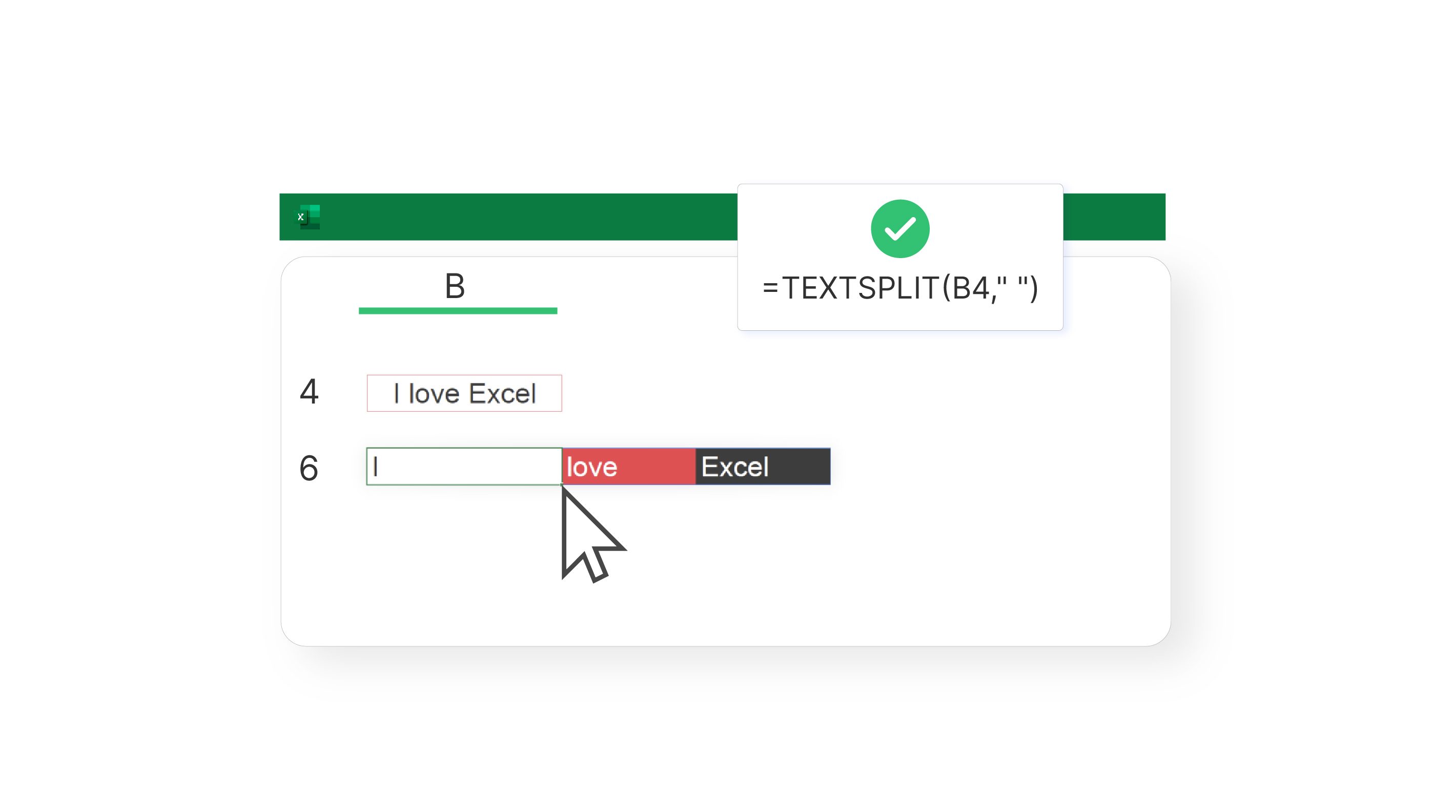
TEXTJOIN has been around for a little while as a text-combining formula… but have you met TEXTJOIN’s new counterpart: TEXTSPLIT?
TEXTSPLIT allows you to split text into multiple columns/rows. Like TEXTJOIN, this new Excel feature uses a given delimiter (i.e. space or comma) to separate the text over the desired cells.
Get familiar with TEXTSPLIT with this helpful content:
- In this blog from Ablebits, Alexander Frolov gives an in-depth tutorial on TEXTSPLIT: TEXTSPLIT function in Excel.
- This blog by Excel Campus compares the merits of TEXTSPLIT to TEXTBEFORE and TEXTAFTER: Best Way to Split Text in Excel.
Excel formula #2: TEXTBEFORE and TEXTAFTER
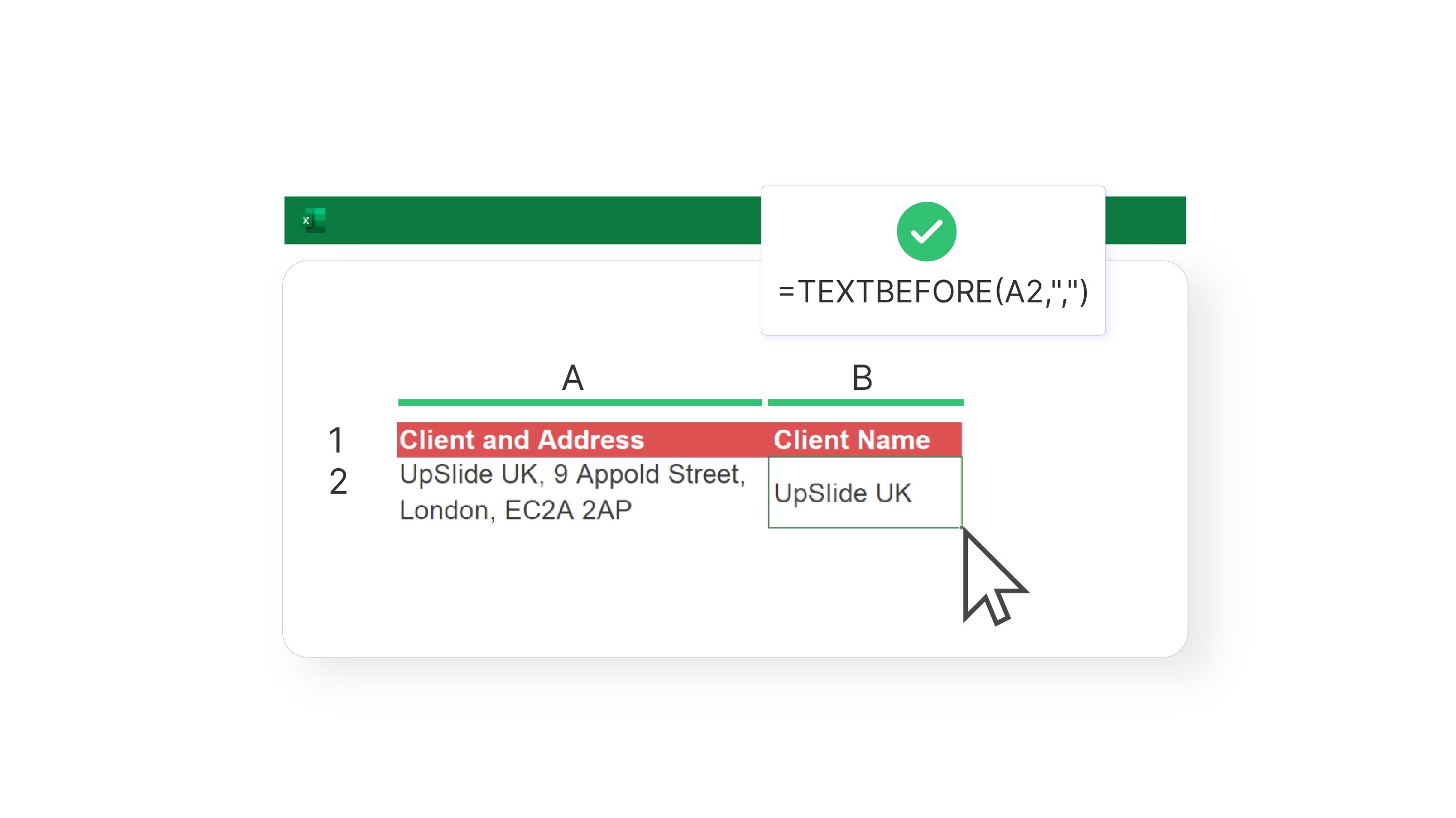
TEXTBEFORE and TEXTAFTER are great tools if you want to extract text from the start or end of a cell. TEXTBEFORE pulls out all text that comes before a given delimiter, while TEXTAFTER does the same with text after that delimiter.
Learn how to leverage these new Excel formulas with these short blogs below:
- This Excel-Exercise blog shows you how to use TEXTBEFORE and TEXTAFTER in just two minutes: TEXTBEFORE and TEXTAFTER.
- Another useful article by Alexander Frolov on how to use TEXTBEFORE: Excel TEXTBEFORE function.
Excel formula #3: TAKE and DROP
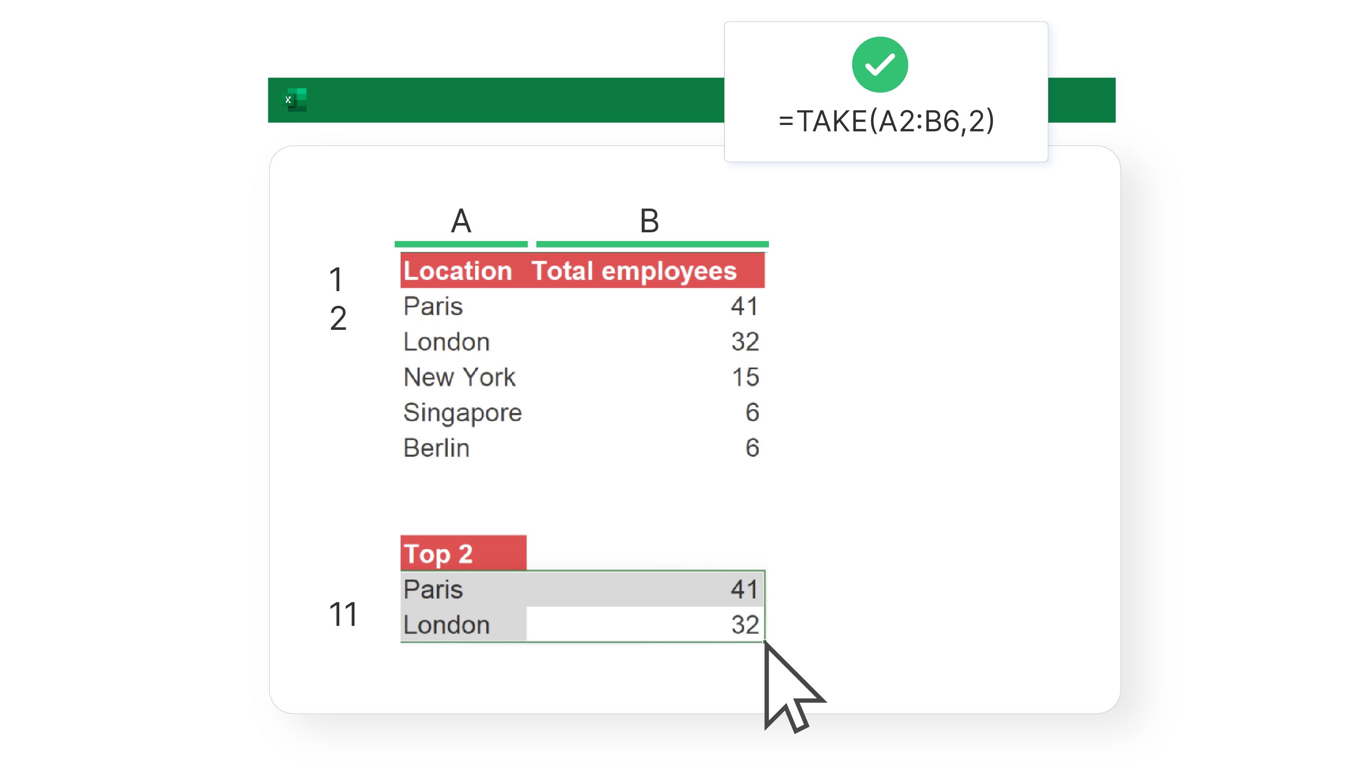
These new Excel features allow you to keep (TAKE) or remove (DROP) a given number of columns/rows from the start or end of an array.
- These tips from Microsoft Support will help you master them in minutes: TAKE function and DROP function.
Excel formula #4: CHOOSECOLS and CHOOSEROWS
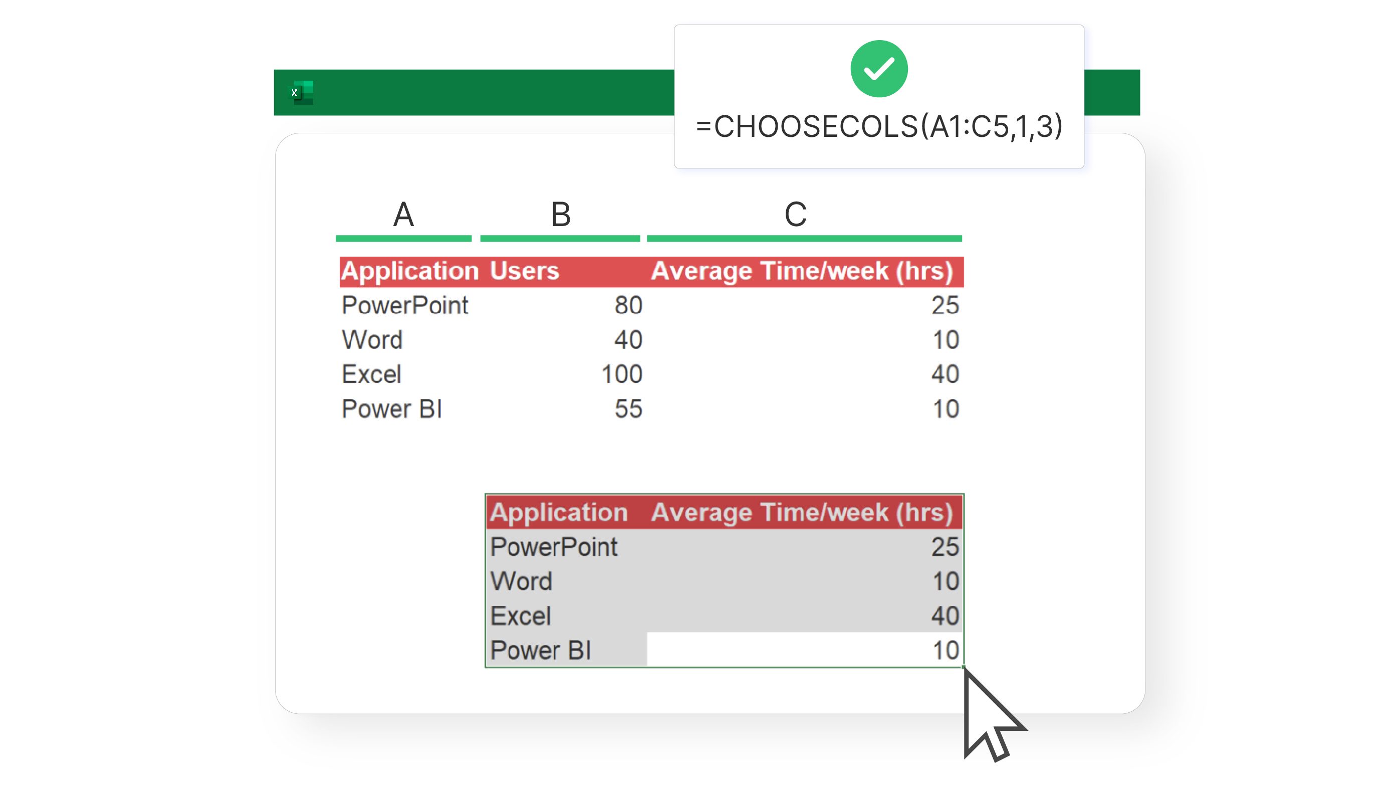
These brand new Excel formulas are an easy way of extracting specific columns (CHOOSECOLS) or rows (CHOOSEROWS) from a range of datasets, whether they’re non-contiguous or right next to each other.
Check out these links to get to grips with CHOOSECOLS and CHOOSEROWS:
- This blog from Get Digital Help gives a quick overview of CHOOSECOLS: How to use the CHOOSECOLS function.
- These Microsoft Support pages are also good for mastering the basics: CHOOSECOLS and CHOOSEROWS.
Excel formula #5: VSTACK and HSTACK
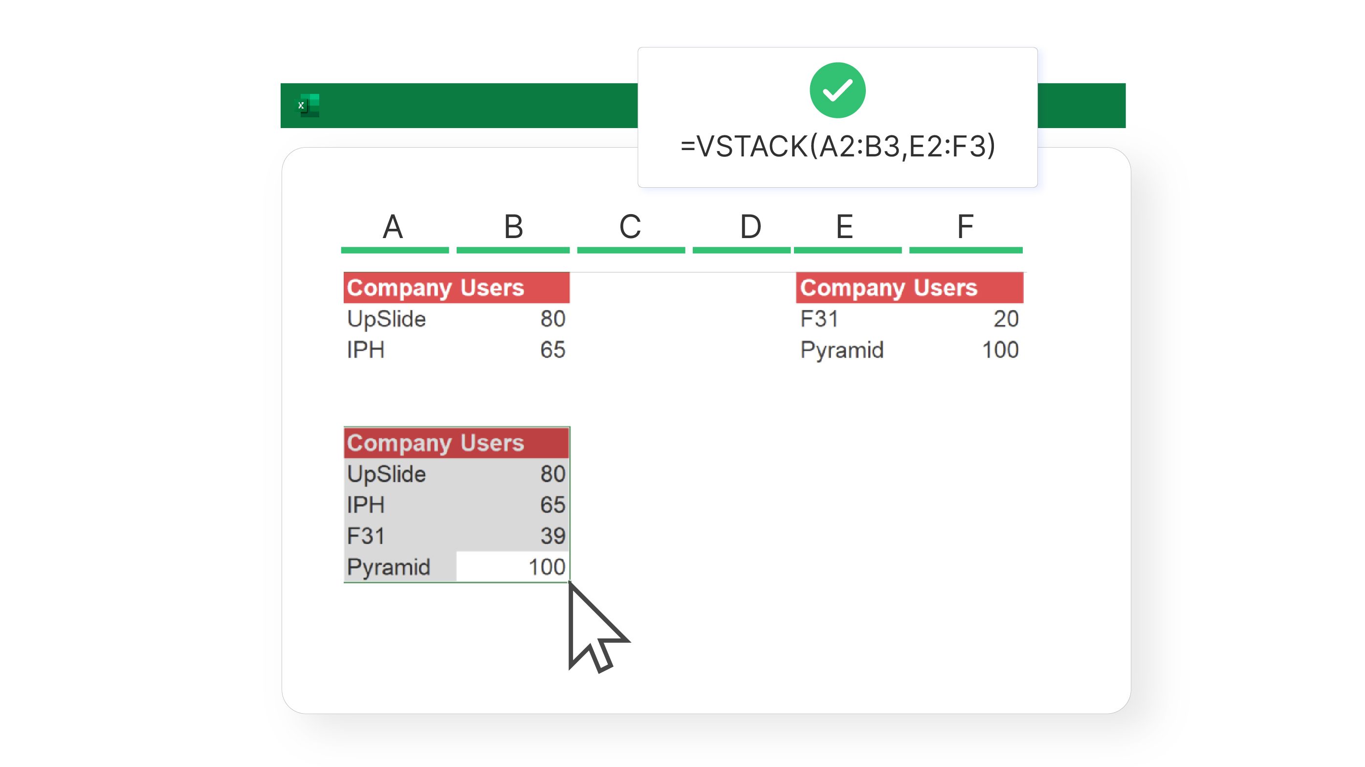
VSTACK and HSTACK allow you to combine two or more sets of arrays vertically (VSTACK) or horizontally (HSTACK). Better yet, these new Excel functions even work with dynamic arrays and ranges with large source sizes!
- For a quick tutorial, these guides from ExtendOffice both go into a lot of detail on each new function: Excel VSTACK function and Excel HSTACK function.
Excel formula #6: XLOOKUP

If you’re an Excel aficionado, you must know the XLOOKUP formula. It’s been available in Office365 and Excel for web since 2020, but we still can’t get enough of this feature in 2022! XLOOKUP is a powerful look-up function that can go far beyond the limitations of VLOOKUP and the INDEX and MATCH functions.
Interested in learning more? Check out these articles below:
- This helpful blog by Inferogroup covers exactly why XLOOKUP is a more efficient function than VLOOKUP: XLOOKUP – The New Improved VLOOKUP.
- This guide from ExcelKid covers 5 common problems with XLOOKUP and how to solve them: 5 Reasons why XLOOKUP is Not Working.
- If you want to go further, you can also watch this video tutorial on XLOOKUP by LinkedIn Learning: Using the XLOOKUP function.
BONUS: Top Excel formulas videos 2022
If you prefer a video tutorial, we’ve also attached our favourite guide to new Excel formulas in 2022 here:
This video is an informative and concise overview of the functions we’ve just covered. Thanks to Mike Tholfsen, you can get to grips with these new Excel functions in just 5 minutes.
What’s your favourite new Excel function? Tell us in the comments below!

This is your one stop shop on learning the new Excel formulas in Office 365: FILTER, RANDARRAY, SEQUENCE, SORT, SORTBY and UNIQUE!
Want to Master the New Excel Formulas in Office 365?
*** Watch our video and step by step guide below with free downloadable Excel workbook to practice ***

FILTER FORMULA
What does it do?
Filters a table array based on the filtering condition given
Formula breakdown:
=FILTER(array, include, [if_empty])
What it means:
=FILTER(data to be filtered, the filtering condition, [value to display if nothing gets matched])
Did you know that you can now filter your table data with an Excel Formula? Yes you can! It is definitely possible now with Excel’s FILTER Formula. It is a new formula introduced in Office 365 released in 2018!
We have a tax table that we want to dynamically filter with a given rate.
I explain how you can do this below:
STEP 1: We need to enter the FILTER function in a blank cell:
=FILTER(

STEP 2: The FILTER arguments:
array
What is the data to be filtered?
Select the cells containing the tax data, do not include the headers:
=FILTER(C9:D14,

include
What is your filtering condition?
We want to filter the tax rate that is greater than the specified rate. Type in the condition as the tax rate column > the specific tax rate.
=FILTER(C9:D14, D9:D14>G8

[if_empty]
What is the value to display in case nothing gets matched?
Just place an empty string to be displayed if nothing gets matched.
=FILTER(C9:D14, D9:D14>G8, “”)

Try it out now with different values and see it get filtered magically!


How to Use the FILTER Formula in Excel
RANDARRAY FORMULA
What does it do?
Creates an array of random numbers
Formula breakdown:
=RANDARRAY([rows], [columns])
What it means:
=RANDARRAY(number of rows, number of columns)
Did you know that you can now generate random numbers in an array? Yes you can! It is definitely possible now with Excel’s RANDARRAY Formula. It is a new formula introduced in Office 365 released in 2018!
It returns random values between 0 and 1 by default. I explain how you can do this below:
STEP 1: We need to enter the RANDARRAY function in a blank cell:
=RANDARRAY(

STEP 2: The RANDARRAY arguments:
[rows]
How many rows to fill random values with?
Let us go for 10 rows.
=RANDARRAY(10,

[columns]
How many columns to fill random values with?
Let us go for 2 columns.
=RANDARRAY(10, 2)

Now we have our 10 x 2 area filled with random values between 0 and 1!

How to Use the RANDARRAY Formula in Excel
SEQUENCE FORMULA
What does it do?
Creates an array of sequential numbers
Formula breakdown:
=SEQUENCE(rows, [columns], [start], [step])
What it means:
=SEQUENCE(number of rows, [number of columns], [starting number], [increment per number])
Did you know that you can now generate a series of numbers with an Excel Formula? Yes you can! It is definitely possible now with Excel’s SEQUENCE Formula. It is a new formula introduced in Office 365 released in 2018!
I explain how you can do this below:
STEP 1: We need to enter the SEQUENCE function in a blank cell:
=SEQUENCE(

STEP 2: The SEQUENCE arguments:
rows
How many rows to fill with values?
Let us go for 10 rows.
=SEQUENCE(10,

[columns]
How many columns to fill with values?
Let us go for 3 columns.
=SEQUENCE(10, 3,

[start]
Which number do you want the sequence of numbers to start?
Let us have it start at the number 10.
=SEQUENCE(10, 3, 10,

[step]
Which increment for each number in the sequence?
Let us increment it by 100. So that numbers should look like: 10, 110, 210, 310, and so on…
=SEQUENCE(10, 3, 10, 100)

Try it out now and see that your sequence of numbers is generated magically!

How to Use the SEQUENCE Formula in Excel
SORT FORMULA
What does it do?
Sorts a table based on a column and order specified
Formula breakdown:
=SORT(array, [sort_index], [sort_order])
What it means:
=SORT(data to be sorted, [which column to be used for sorting], [ascending or descending order])
Did you know that you can now sort your table data with an Excel Formula? Yes you can! It is definitely possible now with Excel’s SORT Formula. It is a new formula introduced in Office 365 released in 2018!
We have a tax table that we want to sort by the tax rate in a descending order.
I explain how you can do this below:
STEP 1: We need to enter the SORT function in a blank cell:
=SORT(

STEP 2: The SORT arguments:
array
What is the data to be sorted?
Select the cells containing the tax data, do not include the headers:
=SORT(C9:D14,

[sort_index]
What is the column to be used for sorting?
We specify the column number here. Since the tax rate column is the second column, place in 2.
=SORT(C9:D14, 2,

[sort_order]
What is the sort order? 1 for Ascending, -1 for Descending order.
Since we want descending order, place in -1.
=SORT(C9:D14, 2, -1)

Now it gets sorted magically!

How to Use the SORT Formula in Excel
SORTBY FORMULA
What does it do?
Sorts a table based on the column(s) specified
Formula breakdown:
=SORTBY(array, by_array1, sort_order1, [by_array2, sort_order2], …)
What it means:
=SORTBY(data to be sorted, by which column to sort first, [by which column to sort afterwards], …)
Did you know that you can now sort your table data with an Excel Formula? Yes you can! It is definitely possible now with Excel’s SORTBY Formula. It also allows you to sort by multiple columns as well. It is a new formula introduced in Office 365 released in 2018!
We have a person list that we want to sort by Gender (ascending order) and then by Age (ascending order).
Do take note that in specifying the sorting order, 1 represents ascending order, -1 represents descending order.
I explain how you can do this below:
STEP 1: We need to enter the SORTBY function in a blank cell:
=SORTBY(

STEP 2: The SORTBY arguments:
array
What is the data to be sorted?
Select the cells containing the person data, do not include the headers:
=SORTBY(B9:D14,

by_array1, sort_order1
Which column will be used to sort first?
Select the cells containing the gender column, then type in 1 for it to be ascending order.
=SORTBY(B9:D14, B9:B14, 1,

by_array2, sort_order2
Which column will be used to sort next?
Select the cells containing the age column, then type in 1 for it to be ascending order.
=SORTBY(B9:D14, B9:B14, 1, D9:D14, 1)

Now it gets sorted magically!

How to Use the SORTBY Formula in Excel
UNIQUE FORMULA
What does it do?
Gets the unique values of a list
Formula breakdown:
=UNIQUE(array)
What it means:
=UNIQUE(data to have duplicates removed)
Want to remove duplicate values from your list? It is definitely possible now with Excel’s UNIQUE Formula. It is a new formula introduced in Office 365 released in 2018!
We have a list of names and we want to remove the duplicates from it. The UNIQUE Formula will make this very quick to do!
I explain how you can do this below:
STEP 1: We need to enter the UNIQUE function in a blank cell:
=UNIQUE(

STEP 2: The UNIQUE arguments:
array
What is the data to be cleared of duplicate values?
Select the cells containing the names, do not include the headers:
=UNIQUE(C9:C14)

Now the duplicate names are all gone!

How to Use the UNIQUE Formula in Excel

What to Know
- To create a formula with references, highlight the cells you want to use, then select an empty cell and enter the formula.
- Enter cell references with pointing. Start the formula with an = sign, select a cell, enter an operator (like + or *), then select another cell.
- Excel calculates results using the BEDMAS rule: Brackets, Exponents, Division and Multiplication, Addition and Subtraction.
This article explains how to create formulas using Microsoft Excel. The instructions apply to Excel 2019, Excel 2016, Excel 2013, Excel 2010, and Excel for Microsoft 365.
Excel Formula Basics
Writing a spreadsheet formula is different from writing an equation in math class. The most notable difference is that Excel formulas start with the equal sign (=) instead of ending with it.
Excel formulas look like =3+2 instead of 3 + 2 =.
The equal sign indicates that what follows is part of a formula and not just a word or number that you want to appear in the cell. After you type the formula and press Enter on your keyboard, the result of the formula appears in the cell.
For example, if you type the formula above, =3+2 into a cell and press Enter, the result, 5, appears in the cell. The formula is still there, but it doesn’t appear in your spreadsheet. If you select the cell, though, the formula appears in the formula bar at the top of the Excel screen.
Improve Formulas with Cell References
Excel formulas can also be developed using cell references. Continuing with our example, you would not enter the numbers 3 and 2, but instead would name cells where these numbers have been entered (see Using Cell References below for more on cell naming). When you write a formula this way, the formula cell always shows the sum of the numbers in those cells, even if the numbers change.
Here’s a real-life example of how this approach can be useful. Say you lead a team of salespeople and are tracking their monthly and quarterly sales. You want to calculate their total sales for the year. Instead of entering every quarterly sales value into a formula, you use cell references to identify the cells where those values can be found within the spreadsheet.
Using Cell References
Each cell in Excel is part of a row and a column. Rows are designated with numbers (1, 2, 3, etc.) shown along the left side of the spreadsheet, while columns are designated with letters (A, B, C, etc.) shown along the top. To refer to a cell, use the column letter and row number together, such as A1 or W22 (the column letter always comes first). If you have a cell selected, you can see its reference at the top of the screen in the Name Box next to the formula bar.
In the image above, notice the cell references in the formula bar: E2, I2, M2, and Q2. They refer to the quarterly sales numbers for the salesperson named Jean. The formula adds those numbers together to come up with the annual sales number. If you update the numbers in one or more of those cells, Excel will recalculate and the result will still be the sum of the numbers in the referred cells.
Create a Formula With Cell References
Try creating a simple formula using cell references.
-
First, you must populate the spreadsheet with data. Open a new Excel file and select cell C1 to make it the active cell.
-
Type 3 in the cell, then press Enter on your keyboard.
-
Cell C2 should be selected. If it’s not, select cell C2. Type 2 in the cell and press Enter on your keyboard.
-
Now create the formula. Select cell D1 and type =C1+C2. Notice that when you type each cell reference, that cell becomes highlighted.
-
Press Enter to complete the formula. The answer 5 appears in cell D1.
If you select cell D1 again, the complete formula =C1+C2 appears in the formula bar above the worksheet.
Enter Cell References With Pointing
Pointing is yet another way to refer to the values you want to include in your formula; it involves using your pointer to select cells to include in your formula. This method is the fastest of those we’ve discussed; it’s also the most accurate because you eliminate the risk of making a mistake in typing in numbers or cell references. Here’s how to do it (starting with the spreadsheet from the examples above):
-
Select cell E1 to make it the active cell and type in the equal sign (=).
-
Use your pointer to select cell C1 to enter the cell reference in the formula.
-
Type a plus sign (+), then use your pointer to select C2 to enter the second cell reference into the formula.
-
Press Enter to complete the formula. The result appears in cell E1.
-
To see how altering one of the formula values alters the result, change the data in cell C1 from 3 to 6 and press Enter on your keyboard. Notice that the results in cells D1 and E1 both change from 5 to 8, though the formulas remain unchanged.
Mathematical Operators and Order of Operations
Now we turn to operations besides addition, including subtraction, division, multiplication, and exponentiation. The mathematical operators used in Excel formulas are similar to those you may remember from math class:
- Subtraction – minus sign ( — )
- Addition – plus sign ( + )
- Division – forward-slash ( / )
- Multiplication – asterisk ( * )
- Exponentiation – caret ( ^ )
If more than one operator is used in a formula, Excel follows a specific order to perform the mathematical operations. An easy way to remember the order of operations is to use the acronym BEDMAS.
- Brackets
- Exponents
- Division
- Multiplication
- Addition
- Subtraction
Excel actually considers division and multiplication to be of equal importance. It performs these operations in the order in which they occur, from left to right. The same is true for addition and subtraction.
Here’s a simple example of the order of operations in use. In the formula =2*(3+2) the first operation Excel completes is the one inside the brackets (3+2), with the result of 5. It then performs the multiplication operation, 2*5, with the result of 10. (The values in the formula could be represented by cell references rather than numbers, but Excel would perform the operations in the same order.) Try entering the formula into Excel to see it work.
Enter a Complex Formula
Now let’s create a more complex formula.
-
Open a new spreadsheet and populate it with data as follows:
- 7 in cell C1
- 5 in cell C2
- 9 in cell C3
- 6 in cell C4
- 3 in cell C5
-
Select cell D1 to make it the active cell and type the equal sign followed by a left bracket (=().
-
Select cell C2 to enter the cell reference in the formula, then type the minus sign (—).
-
Select cell C4 to enter this cell reference into the formula, then type a right bracket ()).
-
Type the multiplication sign (*), then select cell C1 to enter this cell reference into the formula.
-
Type the plus sign (+), then select C3 to enter this cell reference into the formula.
-
Type the division sign (/), then select C5 to enter this cell reference into the formula.
-
Press Enter to complete the formula. The answer -4 appears in cell D1.
How Excel Calculated the Result
In the above example, Excel arrived at the result of -4 using the BEDMAS rules as follows:
- Brackets. Excel first carried out the operation within the brackets, C2-C4 or 5-6 for a result of -1.
- Exponents. There are no exponents in this formula, so Excel skipped this step.
- Division and Multiplication. There are two of these operations in the formula and Excel performed them from left to right. First, it multiplied -1 by 7 (the content of cell C1) to get a result of -7. It then performed the division operation, C3/C5 or 9/3, for a result of 3.
- Addition and Subtraction. The last operation Excel performed was the addition of -7+3 for the final result of -4.
Thanks for letting us know!
Get the Latest Tech News Delivered Every Day
Subscribe
Bottom Line: Learn about the new Dynamic Array functions and formulas that will eventually replace the Ctrl+Shift+Enter array formulas.
Skill Level: Beginner
Video Tutorial
Download the Excel File
Here’s the file I use in the video. Unfortunately, these functions are only available to a portion of users on Microsoft’s Office Insiders Program. So you might not have access just yet. The Insiders program is free for all Office 365 subscribers and gives you access to early release builds and features.
Dynamic Array Functions & Formulas
Microsoft just announced a new feature for Excel that will change the way we work with formulas. The new dynamic array formulas allow us to return multiple results to a range of cells based on one formula. This is called the spill range, and I explain more about it below.
Excel currently has 7 new dynamic array functions, with more on the way. We can use these to create a list of unique values (remove duplicates), sort a list, output a filtered range of data, and so much more. Plus, existing functions can utilize this same spill range functionality.
Goodbye Ctrl+Shift+Enter
The goal of this new functionality is to eventually replace array formulas that we input with Ctrl+Shift+Enter (CSE). Don’t worry, that will be a long goodbye.
CSE formulas are much more complex, and we usually have to guess at how many cells we need to copy them to. Here’s a post and video where I explain more about them.
The image below shows a CSE array formula, enclosed in curly brackets, that can be used to create a list of unique values (remove duplicates).
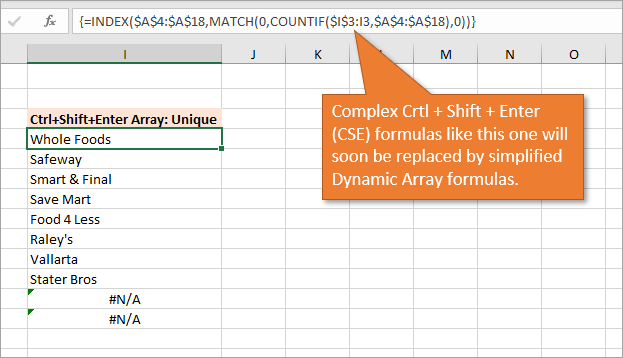
If you don’t have the new functionality yet, checkout this post by my friend Dave at Exceljet on how to the CSE array formula to return unique values.
Let’s take a look at how much easier this will be with the new dynamic array function, UNIQUE.
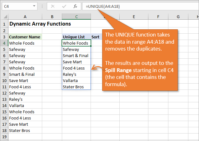
The UNIQUE Function in Excel
With the new UNIQUE function you’ll be able to create a list of unique values (remove duplicate entries) using a very simple formula.
To create a list of unique values, you simply reference the range that contains duplicates in the array argument for UNIQUE.
When the formula is entered, the results will automatically spill down into the cells below.
The UNIQUE function has additional optional arguments as well:
- [by_col] – Allows you to compare by rows or columns when the array is multiple columns wide. Default value is False, to compare by rows.
- [occurs_once] – Allows you to only return values that occur once in the array (range). This is a great option. Default value is False, to return all unique values. Set it to True to return values that only occur once.
Here is the help page on the UNIQUE function to learn more about it.
For those who need to remove duplicates today and don’t have the luxury of waiting for the UNIQUE function to roll out, here’s a post that covers 3 ways to remove duplicates and create a list of unique values.
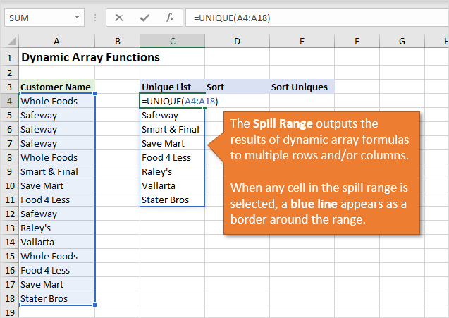
The Spill Range
Get used to the term “spill” for Excel.
The range of cells that contains the results is called the spill range. This range can be multiple rows and/or columns, as you’ll see in the examples below.
The spill range is brand new functionality in Excel that will make our lives much easier. Previously we had to use Ctrl+Shift+Enter array formulas, and try to guess how many cells to copy it to.
Excel is now going to do all that work for us!
When any cell in the spill range is selected, a blue line appears as a border around the range. What happens if something is blocking the spill range?
#SPILL Error
If there is already data in the spill range, a #SPILL error will be returned. This indicates that the range where the results need to spill down is not completely blank.
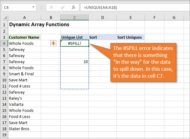
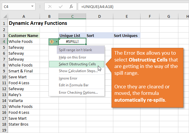
The error box appears and allows you to select the cells that are obstructing the spill range. You can then move or delete those cells, and the formula will automatically re-spill.
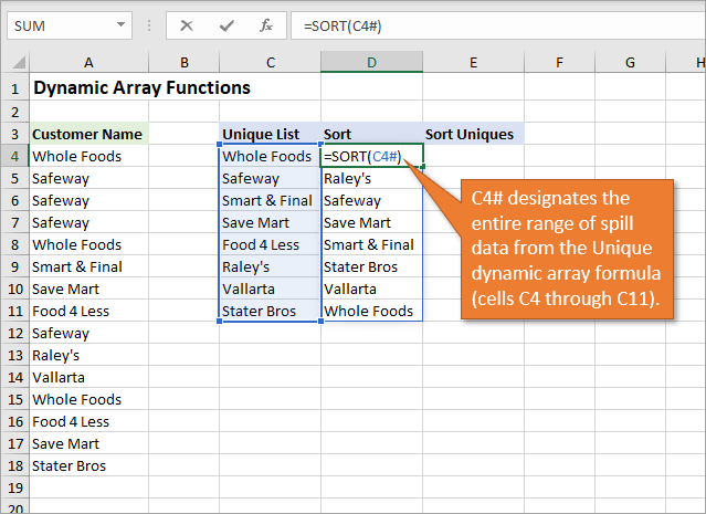
The SORT Function
SORT is another new and very useful function. This outputs a sorted list of the array (range) specified in the function’s first argument.
SORT has additional optional arguments for [sort_index], [sort_order], [by_col]. Here is the help page on the SORT function to learn more.
Spill Reference Notation – Spill Ref
In the example above you’ll notice that I used C4# in the array argument for the SORT function.
This is referred to as a Spill Ref. It allows us to create a reference to the entire spill range by placing a # (hashtag or pound symbol) after the address of the first cell in the spill range.
There are a few ways to create a spill ref:
- Type or select the first cell in a spill range to create a reference to that cell. Then type the # after it. You will see a bounding box appear around the spill range.
- The other way is to select all the cells in the spill range. The spill ref will automatically be created.
- A quick keyboard shortcut for this is to select the first cell in the spill range, then hit Ctrl+Shift+Down Arrow to select all the cells. This automatically creates the spill ref as well.
Uses for Spill Refs
Spill refs are extremely useful. You can use them as the source range for other dynamic array formulas, as I did above with sorting the list of unique values.
You can also use them for regular formulas if you want to do a calculation (SUM, COUNT, etc.) or lookup (VLOOKUP, INDEX, MATCH) on the spill range.
We can even use them for named ranges or data validation (example below). Like I mentioned earlier, spill refs and spill ranges are terms we will use a lot in the future with Excel.
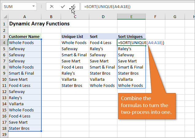
Combining Dynamic Array Functions
Dynamic array functions can also be combined in the same formula. For example, we can use SORT and UNIQUE in the same formula to return a list of sorted unique values.
This is great for the source of a data validation (drop-down) list.
Using Dynamic Arrays for Data Validation Lists
These new formulas can also help to simplify Data Validation (or drop-down) lists in cells.
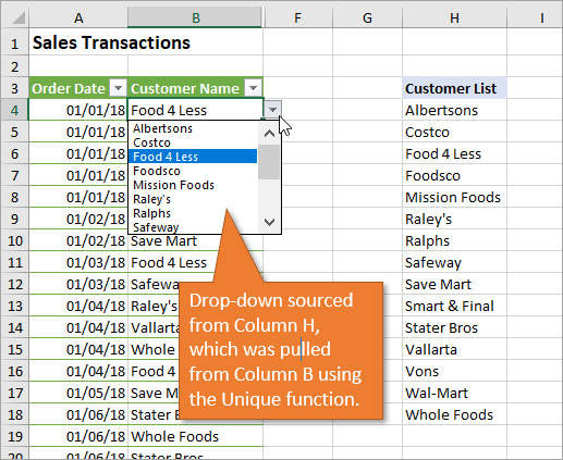
If you are not familiar with Data Validation lists, you can check out my post on the subject here. With this new formula, you can pull out the unique entries from a data set, just as above, and then use that new list as the source of your drop-down list.
In the example below, I used the SORT(UNIQUE()) formula to create a list of uniques from Column B, and output it to Column H. Then I use Column H as the source of my drop-down list for Customer Name.
To do this we can just use a spill ref to reference the spill range (H4#). By adding the hashtag to the end, we are letting Excel know that we want the whole spill range, not just cell H4.
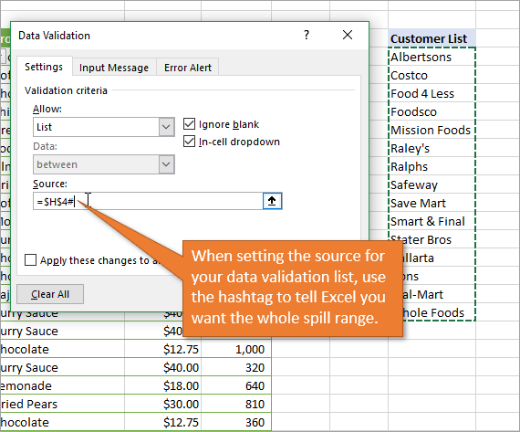
The amazing part is that the spill range automatically updates as items are added to column B. Everything is dynamic, meaning we never need to do maintenance on our ranges or update our formulas. The spill ref always includes everything in the automatically updating spill range.
Filter Function
FILTER is another great function coming to Excel. With the Filter function we can use an entire table as the data source, and filter it down by one or multiple criteria.
For example, in the image below, I’ve filtered the data set on the left to just the information that applies to the customer Stater Bros (cell I1). As I show in the video, the criteria cell(s) can be drop-downs to make for quick interactive reports.
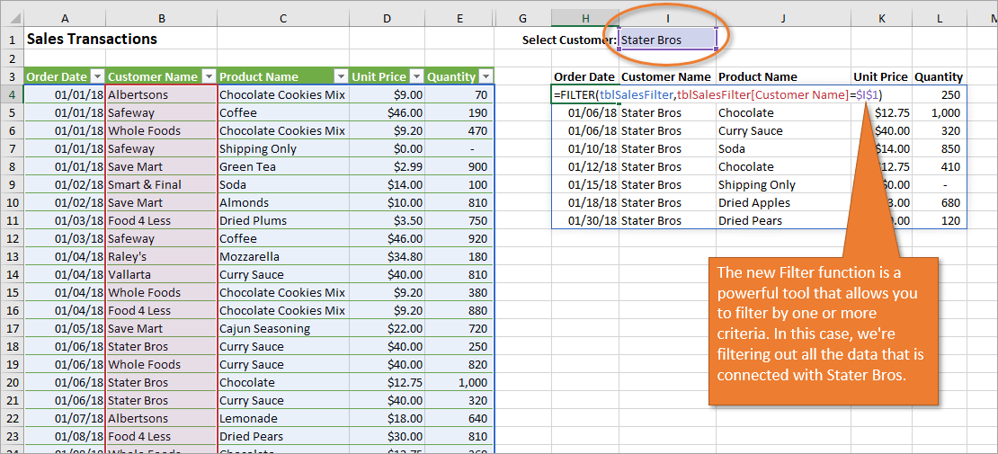
The goal of most array formulas is to do multiple calculations and return multiple results to a range of cells. This FILTER function really demonstrates how a lot can be done with just one simple formula. And again, since these these arrays are dynamic, the results will automatically be updated (re-spilled) any time changes are made to the source range or its precedents.
Dynamic Array Formulas Are Coming!
As I mentioned, these functions are not yet available to the general public. The current availability is limited to a portion of users on Microsoft’s Office Insiders Program (Insider channel). The program is free for Office 365 subscribers. There is no set release date to all Office 365 users yet, but hopefully that will be soon.
As of now, there are 7 new dynamic array functions:
- Filter – allows you to filter a range of data based on criteria you define.
- RandArray – returns an array of random numbers.
- Sequence – allows you to generate a list of sequential numbers in an array, such as 1, 2, 3, 4.
- Sort – sorts the contents of a range or array.
- SortBy – sorts based on the values in a corresponding range or array.
- Unique – returns a list of unique values in a list or range.
- Single – returns a single value at the intersection of a cell’s row or column. Update: The Single function has been removed from Excel and the @ symbol is now used instead for backward compatibility.
You can click any of the links above to read the Microsoft help article about each function.
Existing Functions Can Spill
You might be wondering about other existing array functions in Excel. Well, those functions will spill too. Here is an image of the model I used in my solution on the Dynamic Histogram Chart.
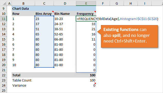
That solutions uses the FREQUENCY function. In older versions of Excel we have to enter that formula with Ctrl+Shift+Enter and first select a range of cells for the output. I had to add extra rows to allow up to 10 bins.
However, with the new spill functionality that setup can actually be simplified. I don’t need all the extra rows with the max number starting in cell C16. I could also use a spill ref for E11# to reference the dynamic range in a named range for the source of my chart. Currently we can’t use spill refs directly in charts, but I’m guessing that will be fixed.
So, the spill range is NOT limited to the new set of functions. We are really getting two new features here: dynamic array functions and spill ranges.
eBook on Dynamic Arrays
Another great resource to learn all about these functions before they release is a new eBook by Bill Jelen. It’s called Excel Dynamic Arrays: Straight to the Point and it’s completely free to download right now for a limited time. The promotional period has ended, but this is still a great resource at a very reasonable price.
Click here to get the eBook
Conclusion
I know, I know, what a jerk right? I get to sit here and tease you about these new features that you probably can’t use yet.
Dynamic arrays are coming soon though. And I hope you’re as excited as I am for this update.
If you have been using Google Sheets, then you know this isn’t really new technology here. However, Excel’s implementation of the spill range and spill refs (A4#) is different (at the time of this writing). It opens up a whole new world of possibility and simplicity with Excel formulas and other features.
You’ve probably heard me say, “there are always a million ways to solve the same problem in Excel…” This new feature probably multiplies that number by another million, leaving us with a lot of new things to explore and learn in Excel. 🙂
I explain how to get these new features in the coming soon section above.
Are you excited for this? Please leave a comment below and let us know. Thank you!