Naming lists in excel

Quick Intro to Excel Named Ranges

One overlooked feature of Microsoft Excel is the ability to create named ranges. A named range is a workbook object that allows you to refer to a cell or a range of cells with a descriptive name rather than a cell reference. When you change the cells that a named range refers to, the formulas that use it are automatically updated. In this tutorial, I’ll show how to name a range in Excel.

Excel Formula Example with Named Range

To show the difference, in our Excel VLOOKUP tutorial, we used:

=VLOOKUP(C2,’Party Codes’!$A$2:$B$45,2,FALSE)

If we named the A2:B45 range on the Party Codes worksheet as “PCODES,” we could instead use:

=VLOOKUP(C2,’Party Codes’!PCODES,2,FALSE)

Besides being easier to read, we no longer have to worry about adding the $ to indicate absolute references. And even though the name makes you think it involves multiple columns, you can name a single cell.

How to Create a Named Range

1. Highlight the Excel range or cell you wish to name.
2. Go to the NAME Box where you normally see the cell address such as A1:
3. Type the NAME you wish to use for the highlighted selection. In our example, we overwrite the A1 cell reference with PCODE. The names are case insensitive.

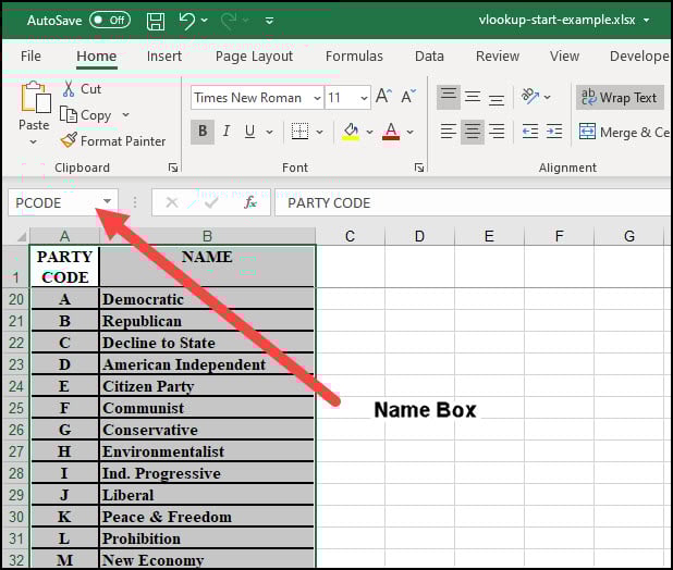Example of named range called “PCODE”

From now on, you can use this PCODE range name in any Excel formula. So, for example, if I created another NAME called “registered,” which included the number of registered voters for each party, I could use a formula such as =SUM(registered). Then, as I type the name, Excel shows it in the drop-down menu with a special icon.

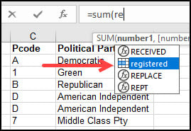Named Range shows with a different icon

You can also jump to this range by clicking the drop-down arrow to the right of the NAME box and selecting your item.

Keyboard Shortcut Method

If you’re a keyboard maven, you may prefer to save some steps and use the keyboard shortcut to create your named range.

1. Highlight your range as normal.
2. Press Ctrl + Shift + F3 .

Create Names from Selection dialog box

1. Press OK.

This will use the Top Row column label of President as the new named range.

Rules for Excel Named Ranges

Yes, most shortcuts usually have rules. Fortunately, there are only four.

1. Your name can’t have spaces. This means I couldn’t use “Political parties.” However, I could use “Political_parties.”
2. Your name can’t be a cell address. I couldn’t use a NAME of “B45” or R45C2 since these are valid Excel cell references.
3. Names can’t be longer than 253 characters.
4. Names can apply to a single worksheet or workbook.

Actually, there is another rule: if you delete a NAME referenced in a formula, it will break. No big surprise there.

Finding and Deleting Named Ranges

If you want to see all the defined names for an Excel workbook, you can find a list in the Name Manager.

1. Click the Formulas tab.
2. Click Name Manager.

Name Manager

1. A dialog appears listing the Name and cell references for each one. You can also delete items from here as well.

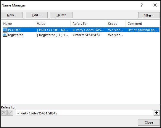List showing existing named ranges

This dialog also allows you to edit a Name or add a descriptive comment.

Another way to access Name Manager is with the keyboard shortcut Ctrl + F3 .

Although we’ve shown names that include a range of cells, you can also use an Excel name for one cell. For example, you might create a name called “election_date” and use it in a formula that computes how many days are left before voting starts. In this scenario, the name is like a constant.

As you can see, Excel’s named ranges are flexible and can make formulas easier to build and interpret. Names also make it easier for other people to learn your workbook. If you want to play around with this feature, you can use the sample Excel file we used for VLOOKUP. Create a name and then change the formula to see how they work.

Источник

Use the Name Manager in Excel

Use the Name Manager dialog box to work with all the defined names and table names in a workbook. For example, you may want to find names with errors, confirm the value and reference of a name, view or edit descriptive comments, or determine the scope. You can also sort and filter the list of names, and easily add, change, or delete names from one location.

To open the Name Manager dialog box, on the Formulas tab, in the Defined Names group, click Name Manager.

The Name Manager dialog box displays the following information about each name in a list box:

One of the following:

A defined name, which is indicated by a defined name icon.

A table name, which is indicated by a table name icon.

Note: A table name is the name for an Excel table, which is a collection of data about a particular subject stored in records (rows) and fields (columns). Excel creates a default Excel table name of Table1, Table2, and so on, each time you insert an Excel table. You can change a table’s name to make it more meaningful. For more information about Excel tables, see Using structured references with Excel tables.

The current value of the name, such as the results of a formula, a string constant, a cell range, an error, an array of values, or a placeholder if the formula cannot be evaluated. The following are representative examples:

«this is my string constant»

The current reference for the name. The following are representative examples:

A worksheet name, if the scope is the local worksheet level.

«Workbook,» if the scope is the global workbook level. This is the default option.

Additional information about the name up to 255 characters. The following are representative examples:

This value will expire on May 2, 2007.

Don’t delete! Critical name!

Based on the ISO certification exam numbers.

The reference for the selected name.

You can quickly edit the range of a name by modifying the details in the Refers to box. After making the change you can click Commit to save changes, or click Cancel to discard your changes.

You cannot use the Name Manager dialog box while you are changing the contents of a cell.

The Name Manager dialog box does not display names defined in Visual Basic for Applications (VBA), or hidden names (the Visible property of the name is set to False).

On the Formulas tab, in the Defined Names group, click Define Name.

In the New Name dialog box, in the Name box, type the name you want to use for your reference.

Note: Names can be up to 255 characters in length.

The scope automatically defaults to Workbook. To change the name’s scope, in the Scope drop-down list box, select the name of a worksheet.

Optionally, in the Comment box, enter a descriptive comment up to 255 characters.

In the Refers to box, do one of the following:

Click Collapse Dialog (which temporarily shrinks the dialog box), select the cells on the worksheet, and then click Expand Dialog .

To enter a constant, type = (equal sign) and then type the constant value.

To enter a formula, type = and then type the formula.

Be careful about using absolute or relative references in your formula. If you create the reference by clicking on the cell you want to refer to, Excel will create an absolute reference, such as «Sheet1!$B$1». If you type a reference, such as «B1», it is a relative reference. If your active cell is A1 when you define the name, then the reference to «B1» really means «the cell in the next column». If you use the defined name in a formula in a cell, the reference will be to the cell in the next column relative to where you enter the formula. For example, if you enter the formula in C10, the reference would be D10, and not B1.

To finish and return to the worksheet, click OK.

Note: To make the New Name dialog box wider or longer, click and drag the grip handle at the bottom.

Источник

How to Create Named Ranges in Excel (A Step-by-step Guide)

What’s in the name?

If you are working with Excel spreadsheets, it could mean a lot of time saving and efficiency.

In this tutorial, you’ll learn how to create Named Ranges in Excel and how to use it to save time.

This Tutorial Covers:

Named Ranges in Excel – An Introduction

If someone has to call me or refer to me, they will use my name (instead of saying a male is staying in so and so place with so and so height and weight).

Similarly, in Excel, you can give a name to a cell or a range of cells.

Now, instead of using the cell reference (such as A1 or A1:A10), you can simply use the name that you assigned to it.

For example, suppose you have a data set as shown below:

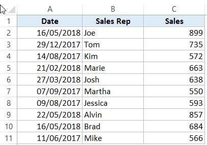
In this data set, if you have to refer to the range that has the Date, you will have to use A2:A11 in formulas. Similarly, for Sales Rep and Sales, you will have to use B2:B11 and C2:C11.

While it’s alright when you only have a couple of data points, but in case you huge complex data sets, using cell references to refer to data could be time-consuming.

Excel Named Ranges makes it easy to refer to data sets in Excel.

You can create a named range in Excel for each data category, and then use that name instead of the cell references. For example, dates can be named ‘Date’, Sales Rep data can be named ‘SalesRep’ and sales data can be named ‘Sales’.

You can also create a name for a single cell. For example, if you have the sales commission percentage in a cell, you can name that cell as ‘Commission’.

Benefits of Creating Named Ranges in Excel

Here are the benefits of using named ranges in Excel.

Use Names instead of Cell References

When you create Named Ranges in Excel, you can use these names instead of the cell references.

For example, you can use =SUM(SALES) instead of =SUM(C2:C11) for the above data set.

Have a look at ṭhe formulas listed below. Instead of using cell references, I have used the Named Ranges.

• Number of sales with value more than 500: =COUNTIF(Sales,”>500″)
• Sum of all the sales done by Tom: =SUMIF(SalesRep,”Tom”,Sales)
• Commission earned by Joe (sales by Joe multiplied by commission percentage):
  =SUMIF(SalesRep,”Joe”,Sales)*Commission

You would agree that these formulas are easy to create and easy to understand (especially when you share it with someone else or revisit it yourself.

No Need to Go Back to the Dataset to Select Cells

Another significant benefit of using Named Ranges in Excel is that you don’t need to go back and select the cell ranges.

You can just type a couple of alphabets of that named range and Excel will show the matching named ranges (as shown below):

Named Ranges Make Formulas Dynamic

By using Named Ranges in Excel, you can make Excel formulas dynamic.

For example, in the case of sales commission, instead of using the value 2.5%, you can use the Named Range.

Now, if your company later decides to increase the commission to 3%, you can simply update the Named Range, and all the calculation would automatically update to reflect the new commission.

How to Create Named Ranges in Excel

Here are three ways to create Named Ranges in Excel:

Method #1 – Using Define Name

Here are the steps to create Named Ranges in Excel using Define Name:

This will create a Named Range SALESREP.

Method #2: Using the Name Box

• Select the range for which you want to create a name (do not select headers).
• Go to the Name Box on the left of Formula bar and Type the name of the with which you want to create the Named Range.
• Note that the Name created here will be available for the entire Workbook. If you wish to restrict it to a worksheet, use Method 1.

Method #3: Using Create From Selection Option

This is the recommended way when you have data in tabular form, and you want to create named range for each column/row.

For example, in the dataset below, if you want to quickly create three named ranges (Date, Sales_Rep, and Sales), then you can use the method shown below.

Here are the steps to quickly create named ranges from a dataset:

This will create three Named Ranges – Date, Sales_Rep, and Sales.

Note that it automatically picks up names from the headers. If there are any space between words, it inserts an underscore (as you can’t have spaces in named ranges).

Naming Convention for Named Ranges in Excel

There are certain naming rules you need to know while creating Named Ranges in Excel:

• The first character of a Named Range should be a letter and underscore character(_), or a backslash(). If it’s anything else, it will show an error. The remaining characters can be letters, numbers, special characters, period, or underscore.
• You can not use names that also represent cell references in Excel. For example, you can’t use AB1 as it is also a cell reference.
• You can’t use spaces while creating named ranges. For example, you can’t have Sales Rep as a named range. If you want to combine two words and create a Named Range, use an underscore, period or uppercase characters to create it. For example, you can have Sales_Rep, SalesRep, or SalesRep.
  • While creating named ranges, Excel treats uppercase and lowercase the same way. For example, if you create a named range SALES, then you will not be able to create another named range such as ‘sales’ or ‘Sales’.
• A Named Range can be up to 255 characters long.

Too Many Named Ranges in Excel? Don’t Worry

Sometimes in large data sets and complex models, you may end up creating a lot of Named Ranges in Excel.

What if you don’t remember the name of the Named Range you created?

Don’t worry – here are some useful tips.

Getting the Names of All the Named Ranges

Here are the steps to get a list of all the named ranges you created:

This will give you a list of all the Named Ranges in that workbook. To use a named range (in formulas or a cell), double click on it.

Displaying the Matching Named Ranges

• If you have some idea about the Name, type a few initial characters, and Excel will show a drop down of the matching names.

How to Edit Named Ranges in Excel

If you have already created a Named Range, you can edit it using the following steps:

Useful Named Range Shortcuts (the Power of F3)

Here are some useful keyboard shortcuts that will come handy when you are working with Named Ranges in Excel:

• To get a list of all the Named Ranges and pasting it in Formula: F3
• To create new name using Name Manager Dialogue Box: Control + F3
• To create Named Ranges from Selection: Control + Shift + F3

Creating Dynamic Named Ranges in Excel

So far in this tutorial, we have created static Named Ranges.

This means that these Named Ranges would always refer to the same dataset.

For example, if A1:A10 has been named as ‘Sales’, it would always refer to A1:A10.

If you add more sales data, then you would have to manually go and update the reference in the named range.

In the world of ever-expanding data sets, this may end up taking up a lot of your time. Every time you get new data, you may have to update the Named Ranges in Excel.

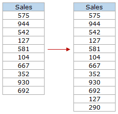
To tackle this issue, we can create Dynamic Named Ranges in Excel that would automatically account for additional data and include it in the existing Named Range.

For example, For example, if I add two additional sales data points, a dynamic named range would automatically refer to A1:A12.

This kind of Dynamic Named Range can be created by using Excel INDEX function. Instead of specifying the cell references while creating the Named Range, we specify the formula. The formula automatically updated when the data is added or deleted.

Let’s see how to create Dynamic Named Ranges in Excel.

Suppose we have the sales data in cell A2:A11.

Here are the steps to create Dynamic Named Ranges in Excel:

1. 1. Go to the Formula tab and click on Define Name.
   2. In the New Name dialogue box type the following:
      • Name: Sales
      • Scope: Workbook
      • Refers to: =$A$2:INDEX($A$2:$A$100,COUNTIF($A$2:$A$100,”<>”&””))
   3. Click OK.

You now have a dynamic named range with the name ‘Sales’. This would automatically update whenever you add data to it or remove data from it.

How does Dynamic Named Ranges Work?

To explain how this work, you need to know a bit more about Excel INDEX function.

Most people use INDEX to return a value from a list based on the row and column number.

But the INDEX function also has another side to it.

It can be used to return a cell reference when it is used as a part of a cell reference.

For example, here is the formula that we have used to create a dynamic named range:

INDEX($A$2:$A$100,COUNTIF($A$2:$A$100,”<>”&””) –> This part of the formula is expected to return a value (which would be the 10th value from the list, considering there are ten items).

However, when used in front of a reference (= $A$2: INDEX($A$2:$A$100,COUNTIF($A$2:$A$100,”<>”&””)) ) it returns the reference to the cell instead of the value.

Hence, here it returns =$A$2:$A$11

If we add two additional values to the sales column, it would then return =$A$2:$A$13

When you add new data to the list, Excel COUNTIF function returns the number of non-blank cells in the data. This number is used by the INDEX function to fetch the cell reference of the last item in the list.

Note:

• This would only work if there are no blank cells in the data.
• In the example taken above, I have assigned a large number of cells (A2:A100) for the Named Range formula. You can adjust this based on your data set.

You can also use OFFSET function to create a Dynamic Named Ranges in Excel, however, since OFFSET function is volatile, it may lead a slow Excel workbook. INDEX, on the other hand, is semi-volatile, which makes it a better choice to create Dynamic Named Ranges in Excel.

You may also like the following Excel resources:

Источник