
Содержание
- Refer to Named Ranges
- Workbook Named Range
- WorkSHEET Specific Named Range
- Referring to a Named Range
- Looping Through Cells in a Named Range
- About the Contributor
- Support and feedback
- Define and use names in formulas
- Name a cell
- Define names from a selected range
- Use names in formulas
- Manage names in your workbook with Name Manager
- Name a cell
- Define names from a selected range
- Use names in formulas
- Manage names in your workbook with Name Manager
- Need more help?
- Ссылка на именованные диапазоны
- Именованный диапазон книги
- Именованный диапазон определенного листа
- Ссылка на именованный диапазон
- Циклический переход по ячейкам в именованном диапазоне
- Об участнике
- Поддержка и обратная связь
- How to Create Named Ranges in Excel (A Step-by-step Guide)
- Named Ranges in Excel – An Introduction
- Benefits of Creating Named Ranges in Excel
- Use Names instead of Cell References
- No Need to Go Back to the Dataset to Select Cells
- Named Ranges Make Formulas Dynamic
- How to Create Named Ranges in Excel
- Method #1 – Using Define Name
- Method #2: Using the Name Box
- Method #3: Using Create From Selection Option
- Naming Convention for Named Ranges in Excel
- Too Many Named Ranges in Excel? Don’t Worry
- Getting the Names of All the Named Ranges
- Displaying the Matching Named Ranges
- How to Edit Named Ranges in Excel
- Useful Named Range Shortcuts (the Power of F3)
- Creating Dynamic Named Ranges in Excel
- How does Dynamic Named Ranges Work?
Refer to Named Ranges
Ranges are easier to identify by name than by A1 notation. To name a selected range, click the name box at the left end of the formula bar, type a name, and then press ENTER.
Note There are two types of named ranges: Workbook Named Range and WorkSHEET Specific Named Range.
Workbook Named Range
A Workbook Named Range references a specific range from anywhere in the workbook (it applies globally).
How to Create a Workbook Named Range:
As explained above, it is usually created entering the name into the name box to the left end of the formula bar. Note that no spaces are allowed in the name.
WorkSHEET Specific Named Range
A WorkSHEET Specific Named Range refers to a range in a specific worksheet, and it is not global to all worksheets within a workbook. Refer to this named range by just the name in the same worksheet, but from another worksheet you must use the worksheet name including «!» the name of the range (example: the range «Name» «=Sheet1!Name»).
The benefit is that you can use VBA code to generate new sheets with the same names for the same ranges within those sheets without getting an error saying that the name is already taken.
How to Create a WorkSHEET Specific Named Range:
- Select the range you want to name.
- Click on the «Formulas» tab on the Excel Ribbon at the top of the window.
- Click «Define Name» button in the Formula tab.
- In the «New Name» dialogue box, under the field «Scope» choose the specific worksheet that the range you want to define is located (i.e. «Sheet1»)- This makes the name specific to this worksheet. If you choose «Workbook» then it will be a WorkBOOK name).
Example, of WorkSHEET Specific Named Range: Selected range to name are A1:A10
Chosen name of range is «name» within the same worksheet refer to the named name mere by entering the following in a cell «=name», from a different worksheet refer to the worksheet specific range by included the worksheet name in a cell «=Sheet1!name».
Referring to a Named Range
The following example refers to the range named «MyRange» in the workbook named «MyBook.xls.»
The following example refers to the worksheet-specific range named «Sheet1!Sales» in the workbook named «Report.xls.»
To select a named range, use the GoTo method, which activates the workbook and the worksheet and then selects the range.
The following example shows how the same procedure would be written for the active workbook.
Sample code provided by: Dennis Wallentin, VSTO & .NET & Excel
This example uses a named range as the formula for data validation. This example requires the validation data to be on Sheet 2 in the range A2:A100. This validation data is used to validate data entered on Sheet 1 in the range D2:D10.
Looping Through Cells in a Named Range
The following example loops through each cell in a named range by using a For Each. Next loop. If the value of any cell in the range exceeds the value of Limit , the cell color is changed to yellow.
About the Contributor
Dennis Wallentin is the author of VSTO & .NET & Excel, a blog that focuses on .NET Framework solutions for Excel and Excel Services. Dennis has been developing Excel solutions for over 20 years and is also the coauthor of «Professional Excel Development: The Definitive Guide to Developing Applications Using Microsoft Excel, VBA and .NET (2nd Edition).»
Support and feedback
Have questions or feedback about Office VBA or this documentation? Please see Office VBA support and feedback for guidance about the ways you can receive support and provide feedback.
Источник
Define and use names in formulas
By using names, you can make your formulas much easier to understand and maintain. You can define a name for a cell range, function, constant, or table. Once you adopt the practice of using names in your workbook, you can easily update, audit, and manage these names.

Name a cell
In the Name Box, type a name.
To reference this value in another table, type th equal sign (=) and the Name, then select Enter.
Define names from a selected range
Select the range you want to name, including the row or column labels.
Select Formulas > Create from Selection.
In the Create Names from Selection dialog box, designate the location that contains the labels by selecting the Top row, Left column, Bottom row, or Right column check box.
Excel names the cells based on the labels in the range you designated.
Use names in formulas
Select a cell and enter a formula.
Place the cursor where you want to use the name in that formula.
Type the first letter of the name, and select the name from the list that appears.
Or, select Formulas > Use in Formula and select the name you want to use.
Manage names in your workbook with Name Manager
On the ribbon, go to Formulas > Name Manager. You can then create, edit, delete, and find all the names used in the workbook.
Name a cell
In the Name Box, type a name.
Define names from a selected range
Select the range you want to name, including the row or column labels.
Select Formulas > Create from Selection.
In the Create Names from Selection dialog box, designate the location that contains the labels by selecting the Top row, Left column, Bottom row, or Right column check box.
Excel names the cells based on the labels in the range you designated.
Use names in formulas
Select a cell and enter a formula.
Place the cursor where you want to use the name in that formula.
Type the first letter of the name, and select the name from the list that appears.
Or, select Formulas > Use in Formula and select the name you want to use.
Manage names in your workbook with Name Manager
On the Ribbon, go to Formulas > Defined Names > Name Manager. You can then create, edit, delete, and find all the names used in the workbook.
In Excel for the web, you can use the named ranges you’ve defined in Excel for Windows or Mac. Select a name from the Name Box to go to the range’s location, or use the Named Range in a formula.
For now, creating a new Named Range in Excel for the web is not available.
Need more help?
You can always ask an expert in the Excel Tech Community or get support in the Answers community.
Источник
Ссылка на именованные диапазоны
Диапазоны легче идентифицировать по имени, чем с помощью нотации A1. Чтобы присвоить имя выбранному диапазону, щелкните поле имени с левой стороны строки формул, введите имя и нажмите клавишу ВВОД.
Примечание Существует два типа именованных диапазонов: именованный диапазон книги и именованный диапазон для таблицы.
Именованный диапазон книги
Именованный диапазон книги относится к определенному диапазону в любом месте книги (применяется глобально).
Как создать именованный диапазон книги:
Как указано выше, обычно он создается путем ввода имени в поле «Имя» с левой стороны строки формул. Обратите внимание, что имя не может содержать пробелов.
Именованный диапазон определенного листа
Именованный диапазон определенного листа относится к диапазону конкретного листа и не является глобальным для всех листов в книге. Ссылайтесь на этот именованный диапазон только по имени на том же листе, но на другом листе необходимо использовать имя листа, включая «!», имя диапазона (например: «Имя» «=Лист1! Имя»).
Преимущество заключается в возможности использования кода VBA для создания новых листов с одинаковыми именами для одних и тех же диапазонов на этих листах без возникновения ошибки, сообщающей, что имя уже используется.
Как создать именованный диапазон определенного листа:
- Выделите диапазон, которому нужно присвоить имя.
- Перейдите на вкладку «Формулы» на ленте Excel в верхней части окна.
- Нажмите кнопку «Присвоить имя» на вкладке формул.
- В диалоговом окне «Создание имени» в поле «Область» выберите конкретный лист, где расположен диапазон, которому нужно присвоить имя (например, «Лист1»), чтобы связать имя с этим листом. Если выбрать вариант «Книга», это будет имя книги.
Пример из worksheet Specific Именованный диапазон: выбранный диапазон для имени A1:A10
Выбранное имя диапазона — «Имя». В пределах одного листа ссылайтесь на именованный диапазон, просто введя в ячейку «=Имя». Из другого листа ссылайтесь на диапазон определенного листа, указав в ячейке имя листа: «= Лист1!Имя».
Ссылка на именованный диапазон
В следующем примере выполняется ссылка на диапазон с именем MyRange в книге с именем MyBook.xls.
В следующем примере выполняется ссылка на диапазон определенного листа с именем Sheet1!Sales в книге с именем Report.xls.
Чтобы выбрать именованный диапазон, используйте метод GoTo, который активирует книгу и лист, а затем выбирает диапазон.
В следующем примере показано, как можно написать эту же процедуру для активной книги.
Пример кода, предоставляемый: Деннис Валлентин(Dennis Wallentin), VSTO & .NET & Excel
В этом примере в качестве формулы для проверки данных используется именованный диапазон. В этом примере данные проверки должны быть на листе 2 в диапазоне A2:A100. Они используются для проверки данных, введенных на листе 1 в диапазоне D2:D10.
Циклический переход по ячейкам в именованном диапазоне
В приведенном ниже примере выполняется циклический переход по каждой ячейке именованного диапазона с помощью цикла For Each. Next. Если значение любой ячейки в диапазоне превышает значение Limit , цвет ячейки изменяется на желтый.
Об участнике
Деннис Валлентин является автором блога VSTO & .NET & Excel, в который основное внимание уделяется решениям платформа .NET Framework для Excel и службы Excel. Деннис разрабатывает решения Excel более 20 лет и также является соавтором книги «Professional Excel Development: The Definitive Guide to Developing Applications Using Microsoft Excel, VBA, and .NET (2nd Edition)».
Поддержка и обратная связь
Есть вопросы или отзывы, касающиеся Office VBA или этой статьи? Руководство по другим способам получения поддержки и отправки отзывов см. в статье Поддержка Office VBA и обратная связь.
Источник
How to Create Named Ranges in Excel (A Step-by-step Guide)
What’s in the name?
If you are working with Excel spreadsheets, it could mean a lot of time saving and efficiency.
In this tutorial, you’ll learn how to create Named Ranges in Excel and how to use it to save time.
This Tutorial Covers:
Named Ranges in Excel – An Introduction
If someone has to call me or refer to me, they will use my name (instead of saying a male is staying in so and so place with so and so height and weight).
Similarly, in Excel, you can give a name to a cell or a range of cells.
Now, instead of using the cell reference (such as A1 or A1:A10), you can simply use the name that you assigned to it.
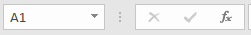
For example, suppose you have a data set as shown below:
In this data set, if you have to refer to the range that has the Date, you will have to use A2:A11 in formulas. Similarly, for Sales Rep and Sales, you will have to use B2:B11 and C2:C11.
While it’s alright when you only have a couple of data points, but in case you huge complex data sets, using cell references to refer to data could be time-consuming.
Excel Named Ranges makes it easy to refer to data sets in Excel.
You can create a named range in Excel for each data category, and then use that name instead of the cell references. For example, dates can be named ‘Date’, Sales Rep data can be named ‘SalesRep’ and sales data can be named ‘Sales’.

You can also create a name for a single cell. For example, if you have the sales commission percentage in a cell, you can name that cell as ‘Commission’.
Benefits of Creating Named Ranges in Excel
Here are the benefits of using named ranges in Excel.
Use Names instead of Cell References
When you create Named Ranges in Excel, you can use these names instead of the cell references.
For example, you can use =SUM(SALES) instead of =SUM(C2:C11) for the above data set.
Have a look at ṭhe formulas listed below. Instead of using cell references, I have used the Named Ranges.
- Number of sales with value more than 500: =COUNTIF(Sales,”>500″)
- Sum of all the sales done by Tom: =SUMIF(SalesRep,”Tom”,Sales)
- Commission earned by Joe (sales by Joe multiplied by commission percentage):
=SUMIF(SalesRep,”Joe”,Sales)*Commission
You would agree that these formulas are easy to create and easy to understand (especially when you share it with someone else or revisit it yourself.
No Need to Go Back to the Dataset to Select Cells
Another significant benefit of using Named Ranges in Excel is that you don’t need to go back and select the cell ranges.
You can just type a couple of alphabets of that named range and Excel will show the matching named ranges (as shown below):

Named Ranges Make Formulas Dynamic
By using Named Ranges in Excel, you can make Excel formulas dynamic.
For example, in the case of sales commission, instead of using the value 2.5%, you can use the Named Range.
Now, if your company later decides to increase the commission to 3%, you can simply update the Named Range, and all the calculation would automatically update to reflect the new commission.
How to Create Named Ranges in Excel
Here are three ways to create Named Ranges in Excel:
Method #1 – Using Define Name
Here are the steps to create Named Ranges in Excel using Define Name:
This will create a Named Range SALESREP.
Method #2: Using the Name Box
- Select the range for which you want to create a name (do not select headers).
- Go to the Name Box on the left of Formula bar and Type the name of the with which you want to create the Named Range.

- Note that the Name created here will be available for the entire Workbook. If you wish to restrict it to a worksheet, use Method 1.

Method #3: Using Create From Selection Option
This is the recommended way when you have data in tabular form, and you want to create named range for each column/row.
For example, in the dataset below, if you want to quickly create three named ranges (Date, Sales_Rep, and Sales), then you can use the method shown below.
Here are the steps to quickly create named ranges from a dataset:
This will create three Named Ranges – Date, Sales_Rep, and Sales.
Note that it automatically picks up names from the headers. If there are any space between words, it inserts an underscore (as you can’t have spaces in named ranges).
Naming Convention for Named Ranges in Excel
There are certain naming rules you need to know while creating Named Ranges in Excel:
- The first character of a Named Range should be a letter and underscore character(_), or a backslash(). If it’s anything else, it will show an error. The remaining characters can be letters, numbers, special characters, period, or underscore.
- You can not use names that also represent cell references in Excel. For example, you can’t use AB1 as it is also a cell reference.
- You can’t use spaces while creating named ranges. For example, you can’t have Sales Rep as a named range. If you want to combine two words and create a Named Range, use an underscore, period or uppercase characters to create it. For example, you can have Sales_Rep, SalesRep, or SalesRep.
- While creating named ranges, Excel treats uppercase and lowercase the same way. For example, if you create a named range SALES, then you will not be able to create another named range such as ‘sales’ or ‘Sales’.
- A Named Range can be up to 255 characters long.
Too Many Named Ranges in Excel? Don’t Worry
Sometimes in large data sets and complex models, you may end up creating a lot of Named Ranges in Excel.
What if you don’t remember the name of the Named Range you created?
Don’t worry – here are some useful tips.
Getting the Names of All the Named Ranges
Here are the steps to get a list of all the named ranges you created:
This will give you a list of all the Named Ranges in that workbook. To use a named range (in formulas or a cell), double click on it.

Displaying the Matching Named Ranges
- If you have some idea about the Name, type a few initial characters, and Excel will show a drop down of the matching names.

How to Edit Named Ranges in Excel
If you have already created a Named Range, you can edit it using the following steps:
Useful Named Range Shortcuts (the Power of F3)
Here are some useful keyboard shortcuts that will come handy when you are working with Named Ranges in Excel:
- To get a list of all the Named Ranges and pasting it in Formula: F3
- To create new name using Name Manager Dialogue Box: Control + F3
- To create Named Ranges from Selection: Control + Shift + F3
Creating Dynamic Named Ranges in Excel
So far in this tutorial, we have created static Named Ranges.
This means that these Named Ranges would always refer to the same dataset.
For example, if A1:A10 has been named as ‘Sales’, it would always refer to A1:A10.
If you add more sales data, then you would have to manually go and update the reference in the named range.
In the world of ever-expanding data sets, this may end up taking up a lot of your time. Every time you get new data, you may have to update the Named Ranges in Excel.
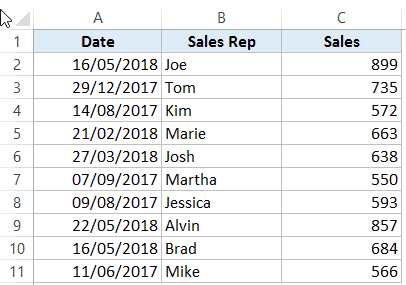
To tackle this issue, we can create Dynamic Named Ranges in Excel that would automatically account for additional data and include it in the existing Named Range.
For example, For example, if I add two additional sales data points, a dynamic named range would automatically refer to A1:A12.
This kind of Dynamic Named Range can be created by using Excel INDEX function. Instead of specifying the cell references while creating the Named Range, we specify the formula. The formula automatically updated when the data is added or deleted.
Let’s see how to create Dynamic Named Ranges in Excel.
Suppose we have the sales data in cell A2:A11.

Here are the steps to create Dynamic Named Ranges in Excel:
-
- Go to the Formula tab and click on Define Name.
- In the New Name dialogue box type the following:
- Name: Sales
- Scope: Workbook
- Refers to: =$A$2:INDEX($A$2:$A$100,COUNTIF($A$2:$A$100,”<>”&””))
- Click OK.
- Go to the Formula tab and click on Define Name.


You now have a dynamic named range with the name ‘Sales’. This would automatically update whenever you add data to it or remove data from it.
How does Dynamic Named Ranges Work?
To explain how this work, you need to know a bit more about Excel INDEX function.
Most people use INDEX to return a value from a list based on the row and column number.
But the INDEX function also has another side to it.
It can be used to return a cell reference when it is used as a part of a cell reference.
For example, here is the formula that we have used to create a dynamic named range:
INDEX($A$2:$A$100,COUNTIF($A$2:$A$100,”<>”&””) –> This part of the formula is expected to return a value (which would be the 10th value from the list, considering there are ten items).
However, when used in front of a reference (= $A$2: INDEX($A$2:$A$100,COUNTIF($A$2:$A$100,”<>”&””)) ) it returns the reference to the cell instead of the value.
Hence, here it returns =$A$2:$A$11
If we add two additional values to the sales column, it would then return =$A$2:$A$13
When you add new data to the list, Excel COUNTIF function returns the number of non-blank cells in the data. This number is used by the INDEX function to fetch the cell reference of the last item in the list.
Note:
- This would only work if there are no blank cells in the data.
- In the example taken above, I have assigned a large number of cells (A2:A100) for the Named Range formula. You can adjust this based on your data set.
You can also use OFFSET function to create a Dynamic Named Ranges in Excel, however, since OFFSET function is volatile, it may lead a slow Excel workbook. INDEX, on the other hand, is semi-volatile, which makes it a better choice to create Dynamic Named Ranges in Excel.
You may also like the following Excel resources:
Источник
November 15, 2015/
Chris Newman
What Is A Named Range?
Creating a named range allows you to refer to a cell or group of cells with a custom name instead of the usual column/row reference. The HUGE benefit to using Named Ranges is it adds the ability to describe the data inside your cells. Let’s look at a quick example:
Can you tell if shipping costs are charged with the product price?
-
= (B7 + B5 * C4) * (1 + A3)
-
=(ShippingCharge + ProductPrice * Quantity) * (1 + TaxRate)
Hopefully, you can clearly see option number TWO gives you immediate insight to whether the cost of the products includes shipping costs. This allows the user to easily understand how the formula is calculating without having to waste time searching through cells to figure out what is what.
How Do I Use Named Ranges?
As a financial analyst, I play around with a bunch of rates. Examples could be anything from a tax rate to an estimated inflation rate. I use named ranges to organize my variables that either are changed infrequently (ie Month or Year) or something that will be static for a good amount of time (ie inflation rate). Here are a list of common names I use on a regular basis:
-
ReportDate
-
Year
-
Month
-
FcstID
-
TaxRate
-
RawData
Creating Unique Names On The Fly
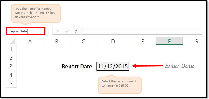
It is super easy to create a Named Range. All you have to do is highlight the cell(s) you want to reference and give it a name in the Name Box. You name cannot have any spaces in it, so if you need to separate words you can either capitalize the beginning of each new word or use an underscore (_). Make sure you hit the ENTER key after you have finished typing the name to confirm the creation of the Named Range.
As a side note, any Named Range created with the Name Box has a Workbook scope. This means the named range can be accessed by any worksheet in your Excel file.
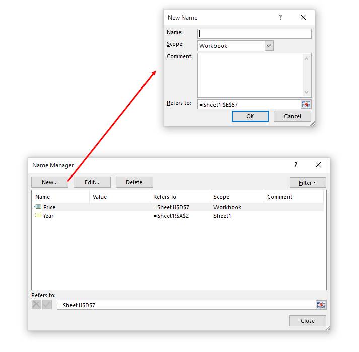
Creating Names With The «Name Manager»
If you want to customize your named ranges even more, you can open up the Name Manager (Formulas tab > Defined Names group > Name Manager button) to edit and create new named ranges.
I won’t go into great detail in this article, but know that with the Name Manager you can
-
Change the name of an existing Named Range
-
Change the reference formula
-
Specify the scope (what worksheets the name can be accessed from)
On To The VBA
Now that you have had a brief overview on Named Ranges, lets dig into some VBA macros you can use to help automate the use of Named Ranges.
Add A Named Range
The below VBA code shows ways you can create various types of named ranges.
Sub NameRange_Add()
‘PURPOSE: Various ways to create a Named Range
‘SOURCE: www.TheSpreadsheetGuru.com
Dim cell As Range
Dim rng As Range
Dim RangeName As String
Dim CellName As String
‘Single Cell Reference (Workbook Scope)
RangeName = «Price»
CellName = «D7»
Set cell = Worksheets(«Sheet1»).Range(CellName)
ThisWorkbook.Names.Add Name:=RangeName, RefersTo:=cell
‘Single Cell Reference (Worksheet Scope)
RangeName = «Year»
CellName = «A2»
Set cell = Worksheets(«Sheet1»).Range(CellName)
Worksheets(«Sheet1»).Names.Add Name:=RangeName, RefersTo:=cell
‘Range of Cells Reference (Workbook Scope)
RangeName = «myData»
CellName = «F9:J18»
Set cell = Worksheets(«Sheet1»).Range(CellName)
ThisWorkbook.Names.Add Name:=RangeName, RefersTo:=cell
‘Secret Named Range (doesn’t show up in Name Manager)
RangeName = «Username»
CellName = «L45»
Set cell = Worksheets(«Sheet1»).Range(CellName)
ThisWorkbook.Names.Add Name:=RangeName, RefersTo:=cell, Visible:=False
End Sub
Loop Through Named Ranges
This VBA macro code shows how you can cycle through the named ranges within your spreadsheet.
Sub NamedRange_Loop()
‘PURPOSE: Delete all Named Ranges in the Active Workbook
‘SOURCE: www.TheSpreadsheetGuru.com
Dim nm As Name
‘Loop through each named range in workbook
For Each nm In ActiveWorkbook.Names
Debug.Print nm.Name, nm.RefersTo
Next nm
‘Loop through each named range scoped to a specific worksheet
For Each nm In Worksheets(«Sheet1»).Names
Debug.Print nm.Name, nm.RefersTo
Next nm
End Sub
Delete All Named Ranges
If you need to clean up a bunch of junk named ranges, this VBA code will let you do it.
Sub NamedRange_DeleteAll()
‘PURPOSE: Delete all Named Ranges in the ActiveWorkbook (Print Areas optional)
‘SOURCE: www.TheSpreadsheetGuru.com
Dim nm As Name
Dim DeleteCount As Long
‘Delete PrintAreas as well?
UserAnswer = MsgBox(«Do you want to skip over Print Areas?», vbYesNoCancel)
If UserAnswer = vbYes Then SkipPrintAreas = True
If UserAnswer = vbCancel Then Exit Sub
‘Error Handler in case Delete Function Errors out
On Error GoTo Skip
‘Loop through each name and delete
For Each nm In ActiveWorkbook.Names
If SkipPrintAreas = True And Right(nm.Name, 10) = «Print_Area» Then GoTo Skip
‘Error Handler in case Delete Function Errors out
On Error GoTo Skip
‘Delete Named Range
nm.Delete
DeleteCount = DeleteCount + 1
Skip:
‘Reset Error Handler
On Error GoTo 0
Next
‘Report Result
If DeleteCount = 1 Then
MsgBox «[1] name was removed from this workbook.»
Else
MsgBox «[» & DeleteCount & «] names were removed from this workbook.»
End If
End Sub
Delete Named Ranges with Error References
This VBA code will delete only Named Ranges with errors in them. These errors can be caused by worksheets being deleted or rows/columns being deleted.
Sub NamedRange_DeleteErrors()
‘PURPOSE: Delete all Named Ranges with #REF error in the ActiveWorkbook
‘SOURCE: www.TheSpreadsheetGuru.com
Dim nm As Name
Dim DeleteCount As Long
‘Loop through each name and delete
For Each nm In ActiveWorkbook.Names
If InStr(1, nm.RefersTo, «#REF!») > 0 Then
‘Error Handler in case Delete Function Errors out
On Error GoTo Skip
‘Delete Named Range
nm.Delete
DeleteCount = DeleteCount + 1
End If
Skip:
‘Reset Error Handler
On Error GoTo 0
Next
‘Report Result
If DeleteCount = 1 Then
MsgBox «[1] errorant name was removed from this workbook.»
Else
MsgBox «[» & DeleteCount & «] errorant names were removed from this workbook.»
End If
End Sub
Anything Missing From This Guide?
Let me know if you have any ideas for other useful VBA macros concerning Named Ranges. Or better yet, share with me your own macros and I can add them to the article for everyone else to see! I look forward to reading your comments below.
About The Author
Hey there! I’m Chris and I run TheSpreadsheetGuru website in my spare time. By day, I’m actually a finance professional who relies on Microsoft Excel quite heavily in the corporate world. I love taking the things I learn in the “real world” and sharing them with everyone here on this site so that you too can become a spreadsheet guru at your company.
Through my years in the corporate world, I’ve been able to pick up on opportunities to make working with Excel better and have built a variety of Excel add-ins, from inserting tickmark symbols to automating copy/pasting from Excel to PowerPoint. If you’d like to keep up to date with the latest Excel news and directly get emailed the most meaningful Excel tips I’ve learned over the years, you can sign up for my free newsletters. I hope I was able to provide you with some value today and I hope to see you back here soon!
— Chris
Founder, TheSpreadsheetGuru.com
Named ranges are one of these crusty old features in Excel that few users understand. New users may find them weird and scary, and even old hands may avoid them because they seem pointless and complex.
But named ranges are actually a pretty cool feature. They can make formulas *a lot* easier to create, read, and maintain. And as a bonus, they make formulas easier to reuse (more portable).
In fact, I use named ranges all the time when testing and prototyping formulas. They help me get formulas working faster. I also use named ranges because I’m lazy, and don’t like typing in complex references 
The basics of named ranges in Excel
What is a named range?
A named range is just a human-readable name for a range of cells in Excel. For example, if I name the range A1:A100 «data», I can use MAX to get the maximum value with a simple formula:
=MAX(data) // max value

The beauty of named ranges is that you can use meaningful names in your formulas without thinking about cell references. Once you have a named range, just use it just like a cell reference. All of these formulas are valid with the named range «data»:
=MAX(data) // max value
=MIN(data) // min value
=COUNT(data) // total values
=AVERAGE(data) // min value
Video: How to create a named range
Creating a named range is easy
Creating a named range is fast and easy. Just select a range of cells, and type a name into the name box. When you press return, the name is created:

To quickly test the new range, choose the new name in the dropdown next to the name box. Excel will select the range on the worksheet.
Excel can create names automatically (ctrl + shift + F3)
If you have well structured data with labels, you can have Excel create named ranges for you. Just select the data, along with the labels, and use the «Create from Selection» command on the Formulas tab of the ribbon:

You can also use the keyboard shortcut control + shift + F3.
Using this feature, we can create named ranges for the population of 12 states in one step:

When you click OK, the names are created. You’ll find all newly created names in the drop down menu next to the name box:

With names created, you can use them in formulas like this
=SUM(MN,WI,MI)
Update named ranges in the Name Manager (Control + F3)
Once you create a named range, use the Name Manager (Control + F3) to update as needed. Select the name you want to work with, then change the reference directly (i.e. edit «refers to»), or click the button at right and select a new range.

There’s no need to click the Edit button to update a reference. When you click Close, the range name will be updated.
Note: if you select an entire named range on a worksheet, you can drag to a new location and the reference will be updated automatically. However, I don’t know a way to adjust range references by clicking and dragging directly on the worksheet. If you know a way to do this, chime in below!
See all named ranges (control + F3)
To quickly see all named ranges in a workbook, use the dropdown menu next to the name box.
If you want to see more detail, open the Name Manager (Control + F3), which lists all names with references, and provides a filter as well:

Note: in older versions of Excel on the Mac, there is no Name Manager, and you’ll see the Define Name dialog instead.
Copy and paste all named ranges (F3)
If you want a more persistent record of named ranges in a workbook, you can paste the full list of names anywhere you like. Go to Formulas > Use in Formula (or use the shortcut F3), then choose Paste names > Paste List:

When you click the Paste List button, you’ll see the names and references pasted into the worksheet:

See names directly on the worksheet
If you set the zoom level to less than 40%, Excel will show range names directly on the worksheet:

Thanks for this tip, Felipe!
Names have rules
When creating named ranges, follow these rules:
- Names must begin with a letter, an underscore (_), or a backslash ()
- Names can’t contain spaces and most punctuation characters.
- Names can’t conflict with cell references – you can’t name a range «A1» or «Z100».
- Single letters are OK for names («a», «b», «x», etc.), but the letters «r» and «c» are reserved.
- Names are not case-sensitive – «home», «HOME», and «HoMe» are all the same to Excel.
Named ranges in formulas
Named ranges are easy to use in formulas
For example, lets say you name a cell in your workbook «updated». The idea is you can put the current date in the cell (Ctrl +  and refer to the date elsewhere in the workbook.

The formula in B8 looks like this:
="Updated: "& TEXT(updated, "ddd, mmmm d, yyyy")
You can paste this formula anywhere in the workbook and it will display correctly. Whenever you change the date in «updated», the message will update wherever the formula is used. See this page for more examples.
Named ranges appear when typing a formula
Once you’ve created a named range, it will appear automatically in formulas when you type the first letter of the name. Press the tab key to enter the name when you have a match and want Excel to enter the name.

Named ranges can work like constants
Because named ranges are created in a central location, you can use them like constants without a cell reference. For example, you can create names like «MPG» (miles per gallon) and «CPG» (cost per gallon) with and assign fixed values:

Then you can use these names anywhere you like in formulas, and update their value in one central location.

Named ranges are absolute by default
By default, named ranges behave like absolute references. For example, in this worksheet, the formula to calculate fuel would be:
=C5/$D$2

The reference to D2 is absolute (locked) so the formula can be copied down without D2 changing.
If we name D2 «MPG» the formula becomes:
=C5/MPG

Since MPG is absolute by default, the formula can be copied down column D as-is.
Named ranges can also be relative
Although named ranges are absolute by default, they can also be relative. A relative named range refers to a range that is relative to the position of the active cell at the time the range is created. As a result, relative named ranges are useful building generic formulas that work wherever they are moved.
For example, you can create a generic «CellAbove» named range like this:
- Select cell A2
- Control + F3 to open Name Manager
- Tab into ‘Refers to’ section, then type: =A1
CellAbove will now retrieve the value from the cell above wherever it is it used.
Important: make sure the active cell is at the correct location before creating the name.
Apply named ranges to existing formulas
If you have existing formulas that don’t use named ranges, you can ask Excel to apply the named ranges in the formulas for you. Start by selecting the cells that contain formulas you want to update. Then run Formulas > Define Names > Apply Names.

Excel will then replace references that have a corresponding named range with the name itself.
You can also apply names with find and replace:

Important: Save a backup of your worksheet, and select just the cells you want to change before using find and replace on formulas.
Key benefits of named ranges
Named ranges make formulas easier to read
The biggest single benefit to named ranges is they make formulas easier to read and maintain. This is because they replace cryptic references with meaningful names. For example, consider this worksheet with data on planets in our solar system. Without named ranges, a VLOOKUP formula to fetch «Position» from the table is quite cryptic:
=VLOOKUP($H$4,$B$3:$E$11,2,0)

However, with B3:E11 named «data», and H4 named «planet», we can write formulas like this:
=VLOOKUP(planet,data,2,0) // position
=VLOOKUP(planet,data,3,0) // diameter
=VLOOKUP(planet,data,4,0) // satellites

At a glance, you can see the only difference in these formulas in the column index.
Named ranges make formulas portable and reusable
Named ranges can make it much easier to reuse a formula in a different worksheet. If you define names ahead of time in a worksheet, you can paste in a formula that uses these names and it will «just work». This is a great way to quickly get a formula working.
For example, this formula counts unique values in a range of numeric data:
=SUM(--(FREQUENCY(data,data)>0))
To quickly «port» this formula to your own worksheet, name a range «data» and paste the formula into the worksheet. As long as «data» contains numeric values, the formula will work straightway.
Tip: I recommend that you create the needed range names *first* in the destination workbook, then copy in the formula as text only (i.e. don’t copy the cell that contains the formula in another worksheet, just copy the text of the formula). This stops Excel from creating names on-the-fly and lets you to fully control the name creation process. To copy only formula text, copy text from the formula bar, or copy via another application (i.e. browser, text editor, etc.).
Named ranges can be used for navigation
Named ranges are great for quick navigation. Just select the dropdown menu next to the name box, and choose a name. When you release the mouse, the range will be selected. When a named range exists on another sheet, you’ll be taken to that sheet automatically.

Named ranges work well with hyperlinks
Named ranges make hyperlinks easy. For example, if you name A1 in Sheet1 «home», you can create a hyperlink somewhere else that takes you back there.


To use a named range inside the HYPERLINK function, add a hash (#) in front of the named range:
=HYPERLINK("#home","take me home")
You can use this same syntax to create a hyperlink to a table:
=HYPERLINK("#Table1","Go to Table1")Note: in older versions of Excel you can’t link to a table like this. However, you can define a name equal to a table (i.e. =Table1) and hyperlink to that.
Named ranges for data validation
Names ranges work well for data validation, since they let you use a logically named reference to validate input with a drop down menu. Below, the range G4:G8 is named «statuslist», then apply data validation with a List linked like this:

The result is a dropdown menu in column E that only allows values in the named range:

Dynamic Named Ranges
Names ranges are extremely useful when they automatically adjust to new data in a worksheet. A range set up this way is referred to as a «dynamic named range». There are two ways to make a range dynamic: formulas and tables.
Dynamic named range with a Table
A Table is the easiest way to create a dynamic named range. Select any cell in the data, then use the shortcut Control + T:

When you create an Excel Table, a name is automatically created (e.g. Table1), but you can rename the table as you like. Once you have created a table, it will expand automatically when data is added.

Dynamic named range with a formula
You can also create a dynamic named range with formulas, using functions like OFFSET and INDEX. Although these formulas are moderately complex, they provide a lightweight solution when you don’t want to use a table. The links below provide examples with full explanations:
- Example of dynamic range formula with INDEX
- Example of dynamic range formula with OFFSET
Table names in data validation
Since Excel Tables provide an automatic dynamic range, they would seem to be a natural fit for data validation rules, where the goal is to validate against a list that may be always changing. However, one problem with tables is that you can’t use structured references directly to create data validation or conditional formatting rules. In other words, you can’t use a table name in conditional formatting or data validation input areas.
However, as a workaround, you can define named a named range that points to a table, and then use the named range for data validation or conditional formatting. The video below runs through this approach in detail.
Video: How to use named ranges with tables
Deleting named ranges
Note: If you have formulas that refer to named ranges, you may want to update the formulas first before removing names. Otherwise, you’ll see #NAME? errors in formulas that still refer to deleted names. Always save your worksheet before removing named ranges in case you have problems and need to revert to the original.
Named ranges adjust when deleting and inserting cells
When you delete *part* of a named range, or if insert cells/rows/columns inside a named range, the range reference will adjust accordingly and remain valid. However, if you delete all of the cells that enclose a named range, the named range will lose the reference and display a #REF error. For example, if I name A1 «test», then delete column A, the name manager will show «refers to» as:
=Sheet1!#REF!
Delete names with Name Manager
To remove named ranges from a workbook manually, open the name manager, select a range, and click the Delete button. If you want to remove more than one name at the same time, you can Shift + Click or Ctrl + Click to select multiple names, then delete in one step.
Delete names with errors
If you have a lot of names with reference errors, you can use the filter button in the name manager to filter on names with errors:

Then shift+click to select all names and delete.
Named ranges and Scope
Named ranges in Excel have something called «scope», which determines whether a named range is local to a given worksheet, or global across the entire workbook. Global names have a scope of «workbook», and local names have a scope equal to the sheet name they exist on. For example, the scope for a local name might be «Sheet2».
The purpose of scope
Named ranges with a global scope are useful when you want all sheets in a workbook to have access to certain data, variables, or constants. For example, you might use a global named range a tax rate assumption used in several worksheets.
Local scope
Local scope means a name is works only on the sheet it was created on. This means you can have multiple worksheets in the same workbook that all use the same name. For example, perhaps you have a workbook with monthly tracking sheets (one per month) that use named ranges with the same name, all scoped locally. This might allow you to reuse the same formulas in different sheets. The local scope allows the names in each sheet to work correctly without colliding with names in the other sheets.
To refer to a name with a local scope, you can prefix the sheet name to the range name:
Sheet1!total_revenue
Sheet2!total_revenue
Sheet3!total_revenue
Range names created with the name box automatically have global scope. To override this behavior, add the sheet name when defining the name:
Sheet3!my_new_name
Global scope
Global scope means a name will work anywhere in a workbook. For example, you could name a cell «last_update», enter a date in the cell. Then you can use the formula below to display the date last updated in any worksheet.
=last_update
Global names must be unique within a workbook.
Local scope
Locally scoped named ranges make sense for worksheets that use named ranges for local assumptions only. For example, perhaps you have a workbook with monthly tracking sheets (one per month) that use named ranges with the same name, all scoped locally. The local scope allows the names in each sheet to work correctly without colliding with names in the other sheets.
Managing named range scope
By default, new names created with the namebox are global, and you can’t edit the scope of a named range after it’s created. However, as a workaround, you can delete and recreate a name with the desired scope.
If you want to change several names at once from global to local, sometimes it makes sense to copy the sheet that contains the names. When you duplicate a worksheet that contains named ranges, Excel copies the named ranges to the second sheet, changing the scope to local at the same time. After you have the second sheet with locally scoped names, you can optionally delete the first sheet.
Jan Karel Pieterse and Charles Williams have developed a utility called the Name Manager that provides many useful operations for named ranges. You can download the Name Manager utility here.