Name of the day of the week in excel

What day of the week is 2019-11-14? Is it a Monday, Tuesday, Wednesday, etc…

It’s pretty common to want to know what day of the week a given date falls on and unless you’ve got some sort of gift for knowing that, you’re going to need a way to figure it out.

In Excel, there are many different ways to determine this. In this post, we’re going to explore 7 ways to achieve this task.

Format a Date as the Weekday Name

The first option we’re going to look at involves formatting our date cells.

Dates in Excel are really just serial numbers starting at 1 for the date 1900-01-01. Formatting is what makes the date look like a date.

There are many ways to format these serial numbers to display the date in various formats like yyyy-mm-dd, dd/mm/yyyy, dd-mmm-yy etc…

One of the possible formatting options for these serial numbers is to display the weekday name with a custom dddd or ddd format.

We can format our dates from the Format Cells dialog box.

1. Select the dates which we want to convert into weekday names.
2. Go to the Home tab and click on the small launch icon in the lower right corner of the Number section. This will open up the Format Cells dialog box. We can also open up the Format Cells dialog a few other ways.
   • The keyboard shortcut Ctrl + 1.
   • Right click on the selected cells ➜ choose Format Cells from the menu.
3. Go to the Number tab in the Format Cells dialog box.
4. Select Custom as the Category.
5. Add dddd into the Type field for the full weekday name or ddd for the abbreviated weekday name.
6. Press the OK button.

Now our dates will appear as the weekday names in the worksheet. The dates are still inside the cells and can be seen in the formula bar when a cell is selected.

Get the Weekday Name with the TEXT Function

The TEXT function will allow us to convert numbers to text and apply formatting to those numbers.

= TEXT ( 1234 , "$#,###" )

We can use the TEXT function to convert the number 1234 into the text string $1,234 with the above formula.

Since dates are really just serial numbers, we can use this function to convert any date into a text string with the weekday name format.

TEXT Syntax

= TEXT ( Value , Format )

• Value (required) is the value to convert to a text string.
• Format (required) is the formatting to apply when converting to a text string.

=TEXT ( B2, "dddd" )

The above formula will convert our date value in cell B2 into the corresponding weekday name. In this example we get a value of Friday from the date 2020-09-18.

Get the Weekday Number with the WEEKDAY Function

While the results aren’t quite as useful, there is also a WEEKDAY function in Excel.

This will convert a date into a corresponding number between 1 and 7 representing the weekday.

WEEKDAY Syntax

= WEEKDAY ( Date , [Type] )

• Date (required) the date to find the weekday number from.

• Type (optional) the weekday number type to return.
  • Omitted or 1 returns 1 for Sunday through 7 for Saturday.
  • 2 returns 1 for Monday through 7 for Sunday.
  • 3 returns 0 for Monday through 6 for Sunday.
  • 11 returns 1 for Monday through 7 for Sunday.
  • 12 returns 1 for Tuesday through 7 for Monday.
  • 13 returns 1 for Wednesday through 7 for Tuesday.
  • 14 returns 1 for Thursday through 7 for Wednesday.
  • 15 returns 1 for Friday through 7 for Thursday.
  • 16 returns 1 for Saturday through 7 for Friday.
  • 17 returns 1 for Sunday through 7 for Saturday.

= WEEKDAY ( B2, 1 )

The above formula will convert our date value in cell B2 into the corresponding weekday number. The second argument value of 1 will return a 1 for Sunday through to 7 for a Saturday. In this case 2019-09-18 returns a 6 because it’s a Friday.

Combining SWITCH with WEEKDAY to Return the Weekday Name

On its own, the WEEKDAY function can only return a number representing the weekday, but we can combine it with the SWITCH function to get the weekday name.

= SWITCH ( WEEKDAY ( B2, 1 ),
	1, "Sun",
	2, "Mon",
	3, "Tue",
	4, "Wed",
	5, "Thu",
	6, "Fri",
	7, "Sat" )

The WEEKDAY function returns a number from 1 to 7 and we can then use the SWITCH function to assign a weekday name to each of these numbers.

Get the WEEKDAY Name Using Power Query

Power Query (also known as Get & Transform) is a powerful data wrangling tool available in Excel 2016 onward.

It makes any data transformation easy and it can get the name of the weekday too.

We first need to import our data into the power query editor. We need our data inside an Excel table.

1. Select a cell inside the Excel table containing the dates.
2. Go to the Data tab in the ribbon.
3. Press the From Table/Range command in the Get & Transform Data section.

This will open up the power query editor.

We can now transform our dates into the name of the weekday.

1. We need to make sure the column is converted to the date data type. Click on the icon in the left of the column heading and select Date from the options.
2. With the date column selected, go to the Add Column tab.
3. Select Date ➜ Day ➜ Name of Day.

= Table.AddColumn( #"Changed Type", "Day Name", each Date.DayOfWeekName( [Date] ), type text )

This will add a new column containing the weekday name and we can see the M code that’s generated in the power query formula bar. This uses the Date.DayOfWeekName power query function.

A similar command can be found in the Transform tab. The difference is, this will not add a new column, but rather transform the selected column.

Get the WEEKDAY Name in a Pivot Table with the WEEKDAY DAX Function

Did you know you can summarize text values with a pivot table?

Well, we can go a step further and summarize our dates as a list of weekday names inside our pivot table using a DAX measure!

We need to create a pivot table from our data.

1. Select a cell inside the data.
2. Go to the Insert tab in the ribbon.
3. Press the PivotTable command.
4. In the Create PivotTable menu check the option to Add this data to the Data Model and press the OK button.

This will create a new blank pivot table in the workbook and add the data into the data model. Adding the data to the data model will allow us to use the DAX formula language with our pivot table.

Now we can create a measure to convert our dates into names and summarize the results into a comma separated list.

1. Select a cell inside the pivot table.
2. Right click on the table in the PivotTable Fields window and select Add Measure from the menu options.

This will open up the DAX formula editor and we can create our DAX measure.

We can now add the following formula into the DAX formula editor.

= CONCATENATEX (
    Activities,
    SWITCH (
        WEEKDAY ( Activities[Date], 1 ),
        1, "Sun",
        2, "Mon",
        3, "Tue",
        4, "Wed",
        5, "Thu",
        6, "Fri",
        7, "Sat"
    ),
    ", "
)

1. Give our new measure a name like Name of Days.
2. Add the above DAX formula into the formula box.

To see the results of our DAX formula, all we need to do is add it into the Values area of our PivotTable Fields window.

This is very similar to the WEEKDAY function solution with Excel functions. The only difference is we need to aggregate the results with a CONCATENATEX function to display inside our pivot table.

Get the Weekday Name in a Pivot Table with the FORMAT DAX Function

Another DAX function we can use to get the weekday name is the FORMAT function. This is very similar to Excel’s TEXT function and will allow us to apply a custom format to our date values.

= CONCATENATEX ( Activities, FORMAT ( Activities[Date], "dddd" ), ", " )

The process is the exact same as the previous DAX example, but instead we create a measure with the above formula.

Get the Weekday Name with a Power Pivot Calculated Column

If you have the power pivot add-in for Excel, then you can use DAX to create a calculated column in the data model.

If our data isn’t already in the data model, we can easily add it by going to the Power Pivot tab in the ribbon ➜ selecting Add to Data Model.

Now we can open up the power pivot window by going to the Power Pivot tab  ➜ selecting Manage Data Model.

= FORMAT ( Activities[Date], "dddd" )

Inside the power pivot window, we can add our new calculated column.

1. Double click on the Add Column heading and give the new column a name like Weekday.
2. Select a cell inside the new column and add the above DAX formula into the formula bar and press enter.

When we close the power pivot window, we now have the new Weekday field available to use in our pivot table and we can add it into the Rows, Columns or Filter area of the pivot table.

Conclusions

There are lots of options to get the name of the day from a date in Excel.

We covered formatting, Excel formulas, power query and DAX formulas in the data model.

There are probably a few more ways as well. Let me know in the comments if I missed your favourite method.

Let’s say you want to see the date displayed for a date value in a cell as «Monday» instead of the actual date of «October 3, 2005.» There are several ways to show dates as days of the week.

Note: The screenshot in this article was taken in Excel 2016. If you have a different version your view might be slightly different, but unless otherwise noted, the functionality is the same.

Format cells to show dates as the day of the week

1. Select the cells that contain dates that you want to show as the days of the week.

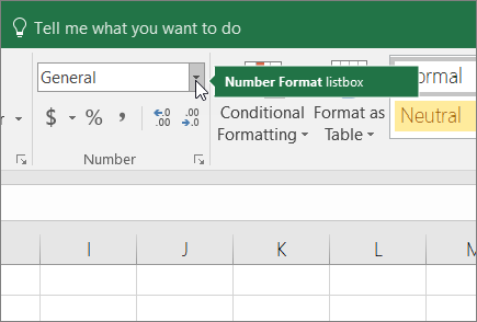
2. On the Home tab, click the dropdown in the Number Format list box, click More Number Formats, and then click the Number tab.

   

3. Under Category, click Custom, and in the Type box, type dddd for the full name of the day of the week (Monday, Tuesday, and so on), or ddd for the abbreviated name of the day of the week (Mon, Tue, Wed, and so on).

Convert dates to the text for the day of the week

To do this task, use the TEXT function.

Example

Copy the following data to a blank worksheet.

1 2 3

A Date 19-Feb-2007 3-Jan-2008 Formula Description (Result) =TEXT(A2, «dddd») Calculates the day of the week for the date and returns the full name of the day of the week (Monday) =TEXT(A3, «ddd») Calculates the day of the week for the date and returns the abbreviated name of the day of the week (Thu)

Need more help?

You can always ask an expert in the Excel Tech Community or get support in the Answers community.

See Also

TEXT

Bottom line: Learn a few different ways to return the name of the day or weekday name for cell that contains a date value.

Skill level: Beginner

In this post we will look at a few different ways to return the day name for a date in Excel.  This can be very useful for creating summary reports, pivot tables, and charts.

Method #1: The Number Format Drop-down Menu

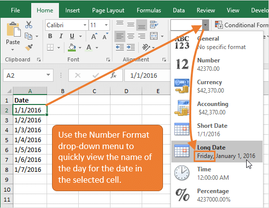
Often times you have a date in a cell and you just want to know the name of the day for the date.  The easiest way to see the weekday name is to select the cell, then press the Number Format Drop-down menu button on the Home tab of the Ribbon.

The Long Date format shows a preview of the date and includes the name of the day for the date in the selected cell.

The keyboard shortcut for the Number Format Drop-down menu is: Alt,H,N,Down Arrow

Checkout my article on how the date system works in Excel to learn more about dates.

Method #2: The Format Cells Dialog Window

We can also see the Long Date format in the Format Cells Window on the Number tab.

This window can be opened by right-clicking the cell, then pressing Format Cells…

The keyboard shortcut for the Format Cells Window is: Ctrl+1

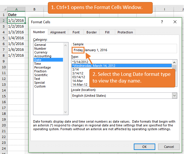
Click on the Long Date format and the Sample box will show a preview that includes the day of the week.

You can also apply a Custom number format to just display the weekday name in the cell.

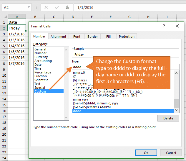
1. Click the Custom category in the Format Cells window.
2. Input one of the following formats in the Type box:
   1. ddd – Returns first three letters of day name (Mon, Tue, Wed, etc.)
   2. dddd – Returns full name of the day (Monday, Tuesday, Wednesday, etc.)
3. Press OK and the cell’s number format will be changed to display the day of the week.

The cell value will still contain the date, but the name of the day will be displayed instead of the date.

Method #3: Use the TEXT Function

The TEXT function is really handy for converting dates to different text formats.  This is great for adding fields to the source data of a pivot table.  It can be used as an alternative to the Date Grouping feature of a pivot table.

The TEXT function contains two arguments.

=TEXT( value, format_text)

• value – The value is a number or date.  In this case we will reference the cell that contains the date.
• format_text – This the the number format that we want to apply to the value.  The number format should be wrapped in quotes. “ddd”

The image below shows that the formula will return the day name of the given date.

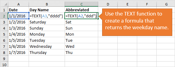
My friend Dave Bruns at ExcelJet has a great article that explains how to use the TEXT function for weekday names in more detail.

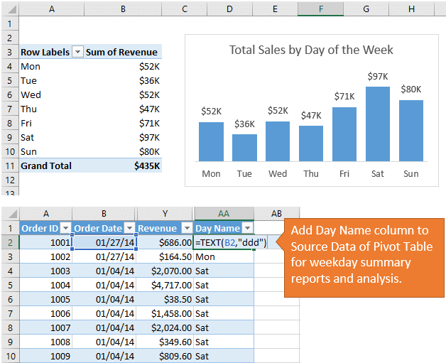
Use the Weekday Name in the Source Data of a Pivot Table

We can then use this technique to add a column to your pivot table source data for the day name.  This basically allows us to group dates by the day of the week.

The example below shows how I used this technique to analyze the sales trend by the day of the week.  With a pivot table you could quickly create a chart or report that shows the total or average sales by weekday for a given period.

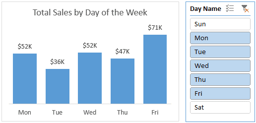
We could also add a slicer with the day name to filter the pivot table or chart.  This would be similar to the technique I explained in the video on how to group days for MTD comparisons.

Checkout my free video series on pivot tables and dashboards to learn more about these great tools in Excel.

What Do You Use the Name of Day For?

Well, there are a few quick tips for getting the name of the day for a date.  Do you have any other ways to get the weekday name?

Please leave a comment below with any questions or suggestions.  Thanks!

At times, you need to find what day of the week is 23-2-2021. It often happens when your data contains dates, months, and years. Is it Sunday, Monday, Tuesday, etc?

Most of the time, you need to get a day of the week from the date in Excel but you don’t know how to do it. You may need to plan daily activities, reports, or another schedule while considering the dates with days. Here, you will find how to get a day of the week from the date in Excel.

Let’s find it out how it happens:

How to Get Day of Week from Date in Excel with the TEXT Function?

The TEXT function in Excel lets you convert numbers to text while applying formatting to the text.

=TEXT (1234, “$#, ###”)

Here you will get to know how the TEXT function is used to convert the number in this syntax 1234 into the text string $1,234.

As you know dates are serial numbers that’s why the TEXT function can easily convert date values into text strings along with the day of the week from date in Excel.

TEXT Syntax

=TEXT (Value, Format)

Value: This is a required argument used to convert the value into a text string.

Format: This is a required argument that helps you in formatting while converting the value to a text string.

=TEXT (B2, “dddd”)

With the help of the above formula, you can easily convert date values in cell B2 to the day of the week. In this example, according to the given data you can see Friday is the day of the week found from the date 18-9-2020.

How to Use Format Cells Feature to Get a Date to Day of Week?

For this function, you don’t need any formula as it needs you to change the format of the date. In the Formula Bar, you can see the date while selecting the cell as well as the day name replaces the date. In case, you don’t want to skip the date value, paste it somewhere else and change the format in the new column. For this, you need to follow these steps:

• Paste the date values into a new column.

• Now, choose the dates in the new column and open the Format Cells dialog box. To open it, you can:
• Press CTRL + 1 or else right-click the cells you have selected and choose Format Cells from the context menu.

• When the Format Cells box opens up, you will see the Number tab, from this tab, select Custom In the Type bar and then choose the formats given below:

ddd: This format gives the first 3 letters of the day of the week.

dddd: It gives the day of the week in the full name.

• Now, click OK.
• You can see the days of the week from the date in Excel here. Whenever you click on a day, it will clearly display the date in the Formula Bar.

How to Get Day of Week from Date in Excel with Number Format Drop-down Menu?

When your data contains dates, you can simply check the name of the day for a particular date. For this, you can simply find the day of the week by selecting the cell. Next, you need to click on the Number Format Drop-down menu option given in the Home tab.

Here, you will see the Long Date format that shows the date and adds the day of week from the date in the selected cell

You can even apply the shortcut command for this operation as well.

ALT + H + N + Down Arrow

Summary:

In this post, you have come to know multiple methods that let you find the day of the week from the date in Excel. Each method is worthy enough to practice that’s why you must try all of them so that you realize which method is suitable for you.

In this example, the goal is to get the day name (i.e. Monday, Tuesday, Wednesday,  etc.) from a given date. There are several ways to go about this in Excel, depending on your needs. This article explains three approaches:

1. Display date with a custom number format
2. Convert date to day name with TEXT function
3. Convert date to day name with CHOOSE function

For all examples, keep in mind that Excel dates are large serial numbers, displayed as dates with number formatting. 

Day name with custom number format

To display a date using only the day name, you don’t need a formula; you can just use a custom number format. Select the date, and use the shortcut Control + 1 to open Format cells. Then select Number > Custom, and enter one of these custom formats:

"ddd"  // i.e."Wed"
"dddd" // i.e."Wednesday"

Excel will display only the day name, but it will leave the date intact. If you want to display both the date and the day name in different columns, one option is to use a formula to pick up a date from another cell, and change the number format to show only the day name. For example, in the worksheet shown, cell F5 contains the date January 1, 2000. The formula in G5, copied down, is:

=F5 // get date from F5

Cells G5 and G6 have the number format «dddd» applied, and cells in G7:G9 have the number format «ddd» applied.

Day name with TEXT function

To convert a date to a text value like «Saturday»,  you can use the TEXT function. The TEXT function is a general function that can be used to convert numbers of all kinds into text values with formatting, including date formats. For example, with the date January 1, 2000 in cell A1, you can use TEXT like this:

=TEXT(A1,"d-mmm-yyyy") // returns "1-Jan-2000"
=TEXT(A1,"mmmm d, yyyy") // returns "January 1, 2000"
=TEXT(A1,"mmmm") // returns "January"

In the worksheet shown, the goal is to display the day name only, so we use a custom number format like «ddd» or «dddd»:

=TEXT(B5,"dddd") // returns "Saturday"
=TEXT(B5,"ddd") // returns "Sat"

Note: The TEXT function converts a date to a text value using the supplied number format. The date is lost in the conversion and only the text for the day name remains.

Day name with CHOOSE function

For maximum flexibility, you can create your own day names with the CHOOSE function. CHOOSE is a general-purpose function for returning a value based on a numeric index. For example, you can use CHOOSE to return one of three colors with a number like this:

=CHOOSE(1,"red","blue","green") // returns "red"
=CHOOSE(2,"red","blue","green") // returns "blue"
=CHOOSE(3,"red","blue","green") // returns "green"

In this example, the goal is to return a day name from a date, so we need to configure CHOOSE to select one of seven-day names. For example, the formula below would return «Wed» based on a numeric index of 4:

=CHOOSE(4,"Sun","Mon","Tue","Wed","Thu","Fri","Sat") // "Wed"

The challenge in this case is to get the right index for a date and for that we need the WEEKDAY function. For any given date, WEEKDAY returns a number between 1-7, which corresponds to the day of the week. By default, WEEKDAY returns 1 for Sunday, 2 for Monday, 3 for Tuesday, etc. In the worksheet shown, the formula in C12 is:

=CHOOSE(WEEKDAY(B12),"Sun","Mon","Tue","Wed","Thu","Fri","Sat")

WEEKDAY returns a number between 1-7, and CHOOSE will use this number to select the corresponding value in the list. Since the date in B12 is January 1, 2000, WEEKDAY returns 7, and CHOOSE returns «Sat».

CHOOSE is more work to set up, but it is also more flexible, since it allows you to convert a date to a day name using any values you want. For example, you can use custom abbreviations or even abbreviations in a different language. In cell C15, CHOOSE is set up to use one letter abbreviations that correspond to Spanish day names:

=CHOOSE(WEEKDAY(B15),"D","L","M","X","J","V","S")

Empty cells

If you use the formulas above on an empty cell, you’ll get «Saturday» as the result. This happens because an empty cell is evaluated as zero, and zero in the Excel date system is the date «0-Jan-1900», which is a Saturday. To work around this issue, you can use the IF function to  return an empty string («»)  for empty cells. For example, if cell A1 may or may not contain a date, you can use IF like this:

=IF(A1<>"",TEXT(A1,"ddd"),"") // check for empty cells

The literal translation of this formula is:  If A1 is not empty, return the TEXT formula, otherwise return an empty string («»).