Name of month excel

Given a date value in Excel, is it possible to extract the month name?

For example, given the 2020-04-23 can you return the value April?

Yes, of course you can! Excel can do it all.

In this post you’ll learn 8 ways you can get the month name from a date value.

Long Date Format

You can get the month name by formatting your dates!

Good news, this is super easy to do!

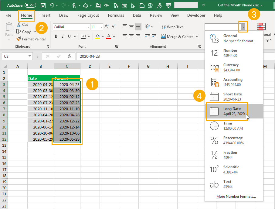
Format your dates:

1. Select the dates you want to format.
2. Go to the Home tab in the ribbon commands.
3. Click on the drop-down in the Numbers section.
4. Select the Long Date option from the menu.

This will format the date 2020-04-23 as April 23, 2020, so you’ll be able to see the full English month name.

This doesn’t change the underlying value in the cell. It is still the same date, just formatted differently.

Custom Formats

This method is very similar to the long date format, but will allow you to format the dates to only show the month name and not include any day or year information.

Select the cells you want to format ➜ right click ➜ select Format Cells from the menu. You can also use the Ctrl + 1 keyboard shortcut to format cells.

In the Format Cells dialog box.

1. Go to the Number tab.
2. Select Custom from the Category options.
3. Enter mmmm into the Type input box.
4. Press the OK button.

This will format the date 2020-04-23 as April, so you’ll only see the full month name with no day or year part.

Again, this formatting won’t change the underlying value, it will just appear differently in the grid.

You can also use the mmm custom format to produce an abbreviated month name from the date such as Apr instead of April.

Flash Fill

Once you’ve formatted a column of date values in the long date format shown above, you’ll be able extract the name into a text value using flash fill.

Start typing a couple examples of the month name in the adjacent column to the formatted dates.

Excel will guess the pattern and fill its guess in a light grey. You can then press Enter to accept these values.

This way the month names will exist as text values and not just formatted dates.

TEXT Function

The previous formatting methods only changed the appearance of the date to show the month name.

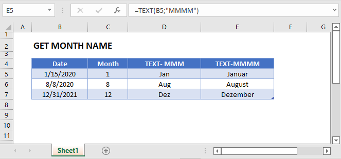
With the TEXT function, you’ll be able to convert the date into a text value.

= TEXT ( B3, "mmmm" )

The above formula will take the date value in cell B3 and apply the mmmm custom formatting. The result will be a text value of the month name.

MONTH Functions

Excel has a MONTH function which can extract the month from a date.

MONTH and SWITCH

This is extracted as a numerical value from 1 to 12, so you will also need to convert that number into a name somehow. To do this you can use the SWITCH function.

= SWITCH (
    MONTH(B3),
    1,"January",
    2,"February",
    3,"March",
    4,"April",
    5,"May",
    6,"June",
    7,"July",
    8,"August",
    9,"September",
    10,"October",
    11,"November",
    12,"December"
)

The above formula is going to get the month number from the date in cell B3 using the MONTH function.

The SWITCH function will then convert that number into a name.

MONTH and CHOOSE

There’s an even more simple way to use the MONTH function as Wayne pointed out in the comments.

You can use the CHOOSE function since the month numbers can correspond to the choices of the CHOOSE function.

= CHOOSE (
    MONTH(B3),
    "January",
    "February",
    "March",
    "April",
    "May",
    "June",
    "July",
    "August",
    "September",
    "October",
    "November",
    "December"
)

The above formula is will get the month number from the date in cell B3 using the MONTH function, CHOOSE then returns the corresponding month name based on the number.

Power Query

You can also use power query to transform your dates into names.

First you will need to convert your data into an Excel table.

Then you can select your table and go to the Data tab and use the From Table/Range command.

This will open up the power query editor where you’ll be able to apply various transformation to your data.

Transform the date column to a month name.

1. Select the column of dates to transform.
2. Go to the Transform tab in the ribbon commands of the power query editor.
3. Click on the Date button in the Date & Time Column section.
4. Choose Month from the Menu.
5. Choose Name of Month from the sub-menu.

This will transform your column of dates into a text value of the full month name.

= Table.TransformColumns ( #"Changed Type", {{"Date", each Date.MonthName(_), type text}} )

This will automatically create the above M code formula for you and your dates will have been transformed.

You can then go to the Home tab and press Close & Load to load the transformed data back into a table in the Excel workbook.

Pivot Table Values

If you have dates in your data and you want to summarize your data by month, then pivot tables are the perfect option.

Select your data then go to the Insert tab and click on the Pivot Table command. You can then choose the sheet and cell to add the pivot table into.

Once you have your pivot table created, you will need to add fields into the Rows and Values area in the PivotTable Fields window.

Drag and drop the Date field into the Rows area and the Sales field into the Values area.

This will automatically create a Months field that summarizes the sales by month in you pivot table and the abbreviated month name will appear in your pivot table.

Power Pivot Calculated Column

You can also create calculated columns with pivot tables and the data model.

This will calculate a value for each row of data and create a new field for use in the PivotTable Fields list.

Follow the same steps as above to insert a pivot table.

In the Create Pivot Table dialog box, check the option to Add this data to the Data Model and press the OK button.

After creating the pivot table, go to the Data tab and press the Manage Data Model command to open the power pivot editor.

= FORMAT ( Table1[Date], "mmmm" )

Create a new column with the above formula inside the power pivot editor.

Close the editor and your new column will be available for use in the PivotTable Fields list.

This calculated column will show up as a new field inside the PivotTable Fields window and you can use it just like any other field in your data.

Conclusions

That’s 8 easy ways to get the month name from a date in Excel.

If you just want to display the name, then the formatting options might be enough.

Otherwise, you can convert the dates into names with flash fill, formulas, power query or even inside a pivot table.

What is your favourite method?

Excel allows you to format dates in many different ways. You can choose to show the date in a short date format or in a long date format.

You can also only show the day number, the month name, or the year from a given date.

In this short Excel tutorial, I will show you some easy methods to get the month name from a date in Excel.

So, let’s get started!

Getting the Month Name from the Date

There are multiple different ways to get monthly from a date in Excel.

The method you choose would depend on how you want the result (i.e., whether you want it as a text string or have the entire date but only show the name of the month)

Let’s see a couple of methods to do this that you can use in different scenarios.

Custom Formatting

Using custom number formatting to get the month name is the best method out of all those covered in this tutorial.

This is because it does not change the underlying date. It only changes the way the date is being displayed in the cell – which is by showing only the month name from the date.

The benefit of using this method is that you can still use the date in calculations.

Suppose you have the dates as shown below and you want to only display the month name and not the entire date.

Below are the steps to do this:

1. Select all the cells that have the dates for which you want to show the month name
2. Click the Home tab
3. In the Number group, click on the dialog box launcher icon (or you can use the keyboard shortcut Control +1). This will open the Format Cells dialog box
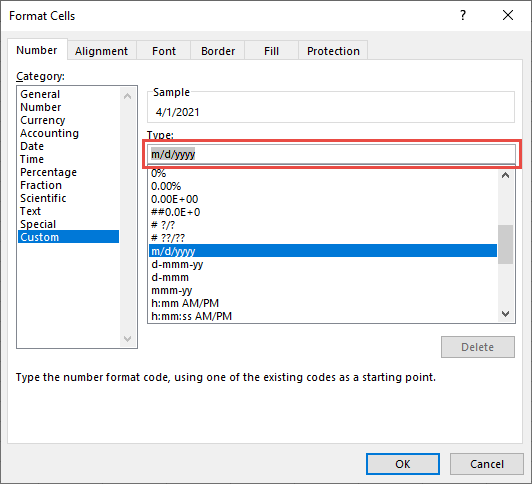
4. In the Category options, click on Custom
5. In the type field, enter – ‘mmmm’. you should see one of the month names in the Sample preview.
6. Click OK

The above steps would convert all the dates into their respective full month names (as shown below).

As I mentioned, the good thing about this method is that even though you are seeing the month names in the cell, the underlying value is still a date (which means that the underlying value is still a number that represents the date).

So, if you want to use these dates in calculations, you can easily do that.

You can also use custom number formatting to show the month name or the month value in different ways. To do this, you will have to give custom number formatting the right code to display the month name.

Below are the different month codes that you can use:

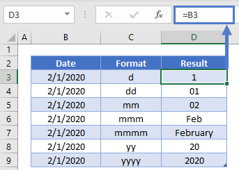
• m – this will show the month number. For example, a date in January would be shown as 1, a date in February would be shown as 2, and so on
• mm – this will also show the month number, but it will also make sure that there are always two digits that are displayed. For example, a date in January would be shown as 01, a date in February would be shown as 02, and a date in November would be shown as 11
• mmm – this will show the month name in a three-letter code. For example, a date in January would be shown as Jan, a date in August would be shown as Aug, and so on
• mmmm – this is the option that we used in the above example, and it would show the complete month name
• mmmmm – this option shows only the first alphabet of the month name. For example, January is shown as J and February is shown as F, and so on. I’ve never seen this being used because it’s confusing as January would also show J and July would also show J

TEXT Function

TEXT function allows us to convert a date into any permissible format that we want and gives the result as a text string.

For example, we can use the TEXT function to show the month name from a date.

Now if you’re wondering how is it different from the custom number formatting we used earlier, the big difference here is that with the TEXT function, you can combine the result with other functions or text strings.

Don’t worry if you are a little lost as of now, the next few examples will make it clear.

Suppose you have a dataset as shown below and you want to show the month name instead of the full date.

Below is the TEXT formula will give you the month name:

=TEXT(A2,"mmmm")

The above text formula takes the date as the input and applies the specified format to it (which is “mmmm” in this formula).

Unlike the Custom Number Formatting method, when you use the TEXT function, the result is a text value. This means that you cannot use the result as a date or number in calculations.

But a good thing about using the TEXT function is that you can combine the result of the function with other text strings.

Let me explain using an example.

Suppose you have the same data set and in this case, instead of just getting the month name, you want to get the month name followed by the quarter number (such as January – Quarter 1).

The below formula would do this for you:

=TEXT(A2,"mmmm")&" - Quarter "&ROUNDUP(MONTH(A2)/3,0)

The above formula uses the ROUNDUP and the MONTH function to get the quarter number of the calendar year, and then it is combined with the month name which is given by the TEXT function.

Since the result of the TEXT function is a text string, I can combine it with other text strings or formula results.

CHOOSE Function

Another formula that you can use to quickly get the month name from the month number is using the CHOOSE formula.

While it ends up being a long formula, the choose formula technique is useful when you want to get the result which you cannot get with custom number formatting or the text function.

For example, if you want to return custom month names (such as month names in any other language or only five alphabets for each month name), you can do that using the CHOOSE formula.

Suppose you have a data set as shown below and you want to get the month name for each of these dates.

Below is the formula that will do that:

=CHOOSE(MONTH(A2),"Jan","Feb","Mar","Apr","May","Jun","Jul","Aug","Sep","Oct","Nov","Dec")

CHOOSE formula takes an index number (which is given by the month formula in our example) and then uses that index number to decide what value to return.

In this example, I have kept the month names to standard three-letter names, but you can change this and use whatever name you want.

Also read: Get Days in Month in Excel

Using Power Query

I have started using Power Query a lot more in my work as I find it a lot easier to clean the data using it.

It has an inbuilt feature that allows you to quickly convert a date into the month name.

The real value of using Power Query in such a scenario would be when you’re importing the data from other Excel files (or consolidating data from multiple Excel files into one file), and while doing it you want to convert your dates into month names.

You can check out my Power Query course on YouTube if you want to learn more about it.

For this technique to work, your data needs to be in an Excel table. While you can still use Power Query with named ranges, if your data is not in an Excel table I recommend you use any of the above methods.

Suppose you have the below data and you want to convert these dates into month names.

Below are the steps to do this:

1. Select any cell in the dataset
2. Click the Data tab
3. In the Get & Transform Data tab, click on From Table/Range
4. In the Power Query editor that opens up, right-click on the Date column header
5. Go to Transform >> Month >> Name of Month
6. Click on Close and Load

The above steps would insert a new worksheet and give you the resulting table in that new sheet.

Now, if you’re wondering why do all this when you can simply use custom number formatting or the text function, you need to understand the real value of Power Query trying to automate work.

If you need the month name from the date just once, feel free to use the methods shown above.

But if you’re using Power Query already to manage data from multiple different sources or combined files or sheets, then knowing that you can easily get the month name from the date can save you a lot of time.

So these are some of the methods that you can use to quickly get the month name from a date in Excel.

I hope you found this tutorial useful.

Other Excel tutorial’s you may also like:

• Calculate the Number of Months Between Two Dates in Excel
• Calculate Time in Excel (Time Difference, Hours Worked, Add/ Subtract)
• How to Change Date Format In Excel?
• How to Get the First Day of the Month in Excel
• How to Add or Subtract Days to a Date in Excel (Shortcut + Formula)
• How to Convert Serial Numbers to Dates in Excel)
• How to Stop Excel from Changing Numbers to Dates Automatically
• How to Make an Interactive Calendar in Excel? (FREE Template)

Dates are an important part of data. There are a few times when we need to use only a part from a date. Take an example of the month. Sometimes you only need a month from a date.

A month is one of the useful components of a date that you can use to summarize data and when it comes to Excel we have different methods to get a month from a date.

I’ve found a total of 5 methods for this. And today, in this post, I’d like to share with you all these methods to get/extract a month from a date. So let’s get down to the business.

1. MONTH Function

Using the MONTH function is the easiest method to extract a month from a date. All you need to do is just refer to a valid date in this function and it will return the number of the month ranging from 1 to 12.

=MONTH(A2)

You can also insert a date directly into the function using the correct date format.

Pro	Con
It’s easy to apply and there is no need to combine it with other functions.	Month number has limited use, most of the time it’s better to present the month name instead of numbers and if you want the month name then you need a different method.

2. TEXT Function

As I said, it’s better to use a month name instead of a month number. Using the TEXT function is a perfect method to extract the month name from a date. The basic work of the text function here is to convert a date into a month by using a specific format.

=TEXT(A2,"MMM")

By default, you have 5 different date formats which you can use in the text function. These formats will return the month name as a text. All you need to do is refer to a date in the function and specify a format. Yes, that’s all. And, make sure the date you are using should be a valid date as per Excel’s date system.

Pros	Cons
You have the flexibility to choose a format among 5 different formats and the original date column will remain the same.	It will return the month name which will be a text and using a custom abbreviation for the month name is not possible.

3. CHOOSE Function

Let’s say you want to get a custom month name or maybe a name in a different language instead of a number or a normal name. In that situation, CHOOSE function can help you. You need to specify a custom name for all 12 months in the function and need to use the month function to get the month number from the date.

=CHOOSE(MONTH(A1),"Jan","Feb","Mar","Apr","May","Jun","Jul","Aug","Sep","Oct","Nov","Dec")

When the month function returns a month number from the date, choose function will return the custom month name instead of that number.

Related: Formula Bar

Pros	Cons
It allows you more flexibility and you can specify a custom month name for each month.	It’s a time-consuming process to add all the values in the function one by one.

4. Power Query

If you want to get a month’s name from a date in a smart way then power query is your calling. It can allow you to convert a date into a month and extract a month number or a month name from a date as well. Power Query is a complete package for you to work with dates. Here you have the below data and here you need months from dates.

• First of all, convert your data into a table.
• After that, select any of the cells from the table and go to the data tab.
• From the data tab, click on “From Table”.

• It will load your table in the power query editor.

From here, you have two different options one is to add a new column with the month name or month number or convert your dates into a month name or month number. Skip the next two steps if you just want to convert your dates into months without adding a new column.

• First of all, right-click on the column heading.
• And after that, click “Duplicate Column”.

• Select the new column from the heading and right-click on it.
• Go to Transform ➜ Month ➜ Name of Month or Month.

• It will instantly convert dates into months.

• Just one more thing, right-click on the column heading and rename the column to “Month”.
• In the end, click on “Close & Load” and it will load your data into a worksheet.

Pro	Con
It’s a dynamic and one-time set-up. Your original data will not get impacted.	You should have a power query in your Excel version and the name of the month will be as a full name.

5. Custom Formatting

If you don’t want to get into any formula method, the simple way you can use it to convert a date into a month is by applying custom formatting. Follow these simple steps.

1. Select the range of cells or the column.
2. Press the shortcut key Ctrl + 1.
3. From the format option, go to “Custom”.
4. Now, in the “Type” input bar enter “MM”, “MMM”, or “MMMMMM”.
5. Click OK.

Pros	Cons
It’s easy to apply and doesn’t change the date but its format.	As the value is a date, when you copy and paste it somewhere else as a value it will be a date, not text. If someone changes the format, the month’s name will be lost.

Conclusion

All the above methods can be used in different situations. But some of them are more frequently used.

TEXT function is applicable in most situations. On the other hand, you also have a power query to get months in a few clicks. If you ask me, I use the text function but these days I am more in love with power query so I would also like to use it.

In the end, I just want to say, you can use any of these methods according to your need. But you need to tell me one thing.

Which one is your favorite method?

Please share with me in the comment section, I’d love to hear from you. And, don’t forget to share this with your friends.

In this example, the goal is to get and display the month name from any given date. There are several ways to go about this in Excel, depending on whether you want to extract the month name as text, or just display a valid Excel using the month name.

To extract the month name from a date as text, you can use the TEXT function with a custom number format like «mmmm», or «mmm». In the example shown, the formula in cell C4 is:

=TEXT(B4,"mmmm") // returns "April"

The TEXT function converts values to text using the number format that you provide. Note that the date is lost in the conversion: only the text for the month name remains. To extract an abbreviated month name like «Jan», «Feb», etc. use a slightly different number format:

=TEXT(B4,"mmm") // returns "Apr"

Display month name

If you only want to display a month name, you don’t need a formula – you can use a custom number format to format the date directly. Select the date and navigate to Format cells (Ctrl + 1 or Cmd +1), then select Custom and enter one of these custom formats:

"mmm"  // "Jan"
"mmmm" // "January"

Excel will display only the month name, but it will leave the date value intact. You can also use a longer date format like this:

"mmmm d, yyyy" // "January 1, 2021

CHOOSE option

For more flexibility, you create your own month names with the CHOOSE function and MONTH function like this:

=CHOOSE(MONTH(date),"Jan","Feb","Mar","Apr","May","Jun","Jul","Aug","Sep","Oct","Nov","Dec")

Enter the month names you want to return (customized as you like) as values in CHOOSE, after the first argument, which is entered as MONTH(date). The MONTH function will extract a month number, and CHOOSE will use this number to return the «nth» value in the list. This works because MONTH returns a number 1-12 that corresponds to the month name.

CHOOSE is more work to set up, but it is also more flexible, since it allows you to map a date to any values you want (i.e. you can use values that are custom, abbreviated, not abbreviated, in a different language, etc.).

Return to Excel Formulas List

Download Example Workbook

Download the example workbook

This tutorial will demonstrate how to get the name of a month from a date in Excel and Google Sheets.

Get Month Number Using Month Function

If you only need the month number from a date, you can calculate this by using the Month Function:

=MONTH(B3)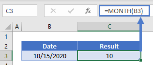

Get Month Name with TEXT Function

Text – Month

If you need to calculate the month name, you can use the TEXT Function:

=TEXT(B3,"mmmm")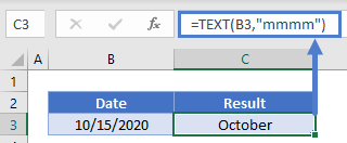

The TEXT Function will return the month name when you enter text format “mmmm”. Below we will demonstrate more text formats to use.

Choose Month

Depending on your purpose, you may also use the CHOOSE Function to calculate the month name of a date:

=CHOOSE(MONTH(B3),"Jan","Feb","Mar","Apr","May","Jun","Jul","Aug","Sep","Oct","Nov","Dec")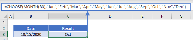

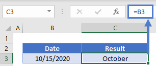
Get Month By Changing Formatting

In the previous examples, the output cell returns text containing the month name. Instead, you can simply change the formatting of the date to display only the month name. This will keep all the properties of the date, while only showing the month.

By changing a date’s Date Format to “MMMM” you can see the month name:

or “MMM” to see the month abbreviation:

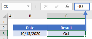
Note: This will display the month name, but the value stored in the cell will still be the date.

Change Number Format

To change the number format follow these steps:

Open the Number Tab of the Cell Formatting menu. This can be accessed with the shortcut CTRL + 1 or by clicking this button on the Home Ribbon:

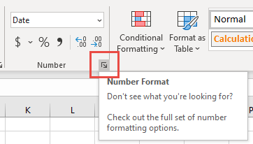
Next navigate to the Custom section.

The Custom section of the Format Cells Menu allows you the ability to create your own number formats:

To set custom number formatting for dates, you’ll need to specify how to display days, months, and / or years. Use this table as guide:

Notice you can use “mmm” or “mmmm” to display the month name.

Get Month Name in Google Sheets

You can calculate the month name of a date the same in Google Sheets as in Excel: