
If you work with formulas in Excel, sooner or later you will encounter the problem where Excel formulas don’t work at all (or give the wrong result).
While it would have been great had there been only a few possible reasons for malfunctioning formulas. Unfortunately, there are too many things that can go wrong (and often does).
But since we live in a world that follows the Pareto principle, if you check for some common issues, it’s likely to solve 80% (or maybe even 90% or 95% of the issues where formulas are not working in Excel).
And in this article, I will highlight those common issues that are likely the cause of your Excel formulas not working.
So let’s get started!
Incorrect Syntax of the Function
Let me start by pointing out the obvious.
Every function in Excel has a specific syntax – such as the number of arguments it can take or the type of arguments it can accept.
And in many cases, the reason your Excel formulas are not working or gives the wrong result could be an incorrect argument (or missing arguments).
For example, the VLOOKUP function takes three mandatory arguments and one optional argument.
If you provide a wrong argument or don’t specify the optional argument (where it’s needed for the formula to work), it’s going to give you a wrong result.
For example, suppose you have a dataset as shown below where you need to know the score of Mark in Exam 2 (in cell F2).

If I use the below formula, I will get the wrong result, because I am using the wrong value in the third argument (one that asks for Column Index number).
=VLOOKUP(A2,A2:C6,2,FALSE)

In this case, the formula calculates (as it returns a value), but the result is incorrect (instead of score in Exam 2, it gives the score in Exam 1).
Another example where you need to be cautious about the arguments is when using VLOOKUP with the approximate match.
Since you need to use an optional argument to specify where you want VLOOKUP to do an exact match or an approximate match, not specifying this (or using the wrong argument) can cause issues.
Below is an example where I have the marks data for some students and I want to extract marks in Exam 1 for the students in the table on the right.

When I use the below VLOOKUP formula it gives me an error for some names.
=VLOOKUP(E2,$A$2:$C$6,2)

This happens as I have not specified the last argument (which is used to determine whether to do an exact match or approximate match). When you don’t specify the last argument, it automatically does an approximate match by default.
Since we needed to do an exact match in this case, the formula returns an error for some names.
While I have taken the example of the VLOOKUP function, in this case, this is something that can be applicable for many Excel formulas that have optional arguments as well.
Also read: Identify Errors Using Excel Formula Debugging
Extra Spaces Causing Unexpected Results
Leading, trailing spaces are hard to find out and can cause issues when you use a cell that has these in formulas.
For example, in the below example, if I try to use VLOOKUP to fetch the score for Mark, it gives me the #N/A error (the not available error).

While I can see that the formula is correct and the name ‘Mark’ is clearly there is the list, what I can not see is that there is a trailing space in the cell that has the name (in cell D2).

Excel doesn’t consider the content of these two cells the same and therefore it considers it a mismatch when fetching the value using VLOOKUP (or it could be any other lookup formula).
To fix this issue, you need to remove these extra space characters.
You can do this by using any of the following methods:
- Clean the cell and remove any leading/trailing spaces before using it in formulas
- Use the TRIM function within the formula to make sure any leading/trailing/double spaces are ignored.
In the above example, you can use the below formula instead to make sure it works.
=VLOOKUP(TRIM(D2),$A$2:$B$6,2,0)
While I have taken the VLOOKUP example, this is also a common issue when working with TEXT functions.
For example, if I use the LEN function to count the total number of characters in a cell, if there are leading or trailing spaces, these would also be counted and give the wrong result.
Take away / How to Fix: If possible, clean your data by removing any leading/trailing or double spaces before using these in formulas. If you can not change the original data, use the TRIM function in formulas to take care of this.
Using Manual Calculation Instead of Automatic
This one setting can drive you crazy (if you don’t know it’s what’s causing all the issues).
Excel has two calculation modes – Automatic and Manual.
By default, the automatic mode is enabled, which means that in case I use a formula or make any changes in the existing formulas, it automatically (and instantly) makes the calculation and gives me the result.
This is the setting we are all used to.
In the automatic setting, whenever you make any change in the worksheet (such as entering a new formula to even some text in a cell), Excel automatically recalculates everything (yes, everything).
But in some cases, people enable the manual calculation setting.
This is mostly done when you have a heavy Excel file with a lot of data and formulas. In such cases, you may not want Excel to recalculate everything when you make small changes (as it may take a few seconds or even minutes) for this recalculation to complete.
If you enable manual calculation, Excel will not calculate unless you force it to.
And this may make you think that your formula is not calculating.
All you need to do in this case is either set the calculation back to automatic or force a recalculation by hitting the F9 key.
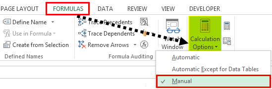
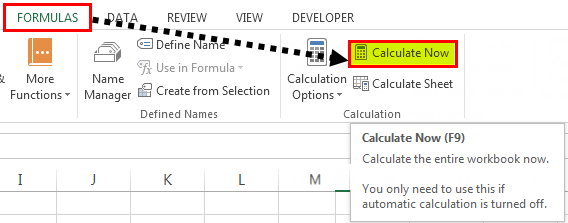
Below are the steps to change the calculation from manual to automatic:
- Click the Formula tab

- Click on Calculation Options
- Select Automatic


Important: In case you’re changing the calculation from manual to automatic, it’s a good idea to create a backup of your workbook (just in case this makes your workbook hang or makes Excel crash)
Take away / How to Fix: If you notice that your formulas are not giving the expected result, try something simple in any cell (such as adding 1 to an existing formula. Once you identify the issue as the one where calculation mode needs to be changed, do a force calculation by using F9.
Deleting Rows/Column/Cells Leading to #REF! Error
One of the things that can have a devastating effect on your existing formulas in Excel is when you delete any row/column which has been used in calculations.
When this happens, sometimes, Excel adjusts the reference itself and makes sure that the formulas are working fine.
And sometimes… it can not.
Thankfully, one clear indication that you get when formulas break on deleting cells/rows/columns is the #REF! error in the cells. This is a reference error that tells you that there is some issue with the references in the formula.
Let me show you what I mean by using an example.
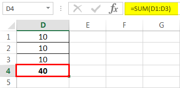
Below I have used the SUM formula to add the cells A2:A6.

Now, if I delete any of these cells/rows, the SUM formula will return a #REF! error. This happens because when I deleted the row, the formula doesn’t know what to reference now.
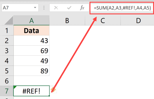
You can see that the third argument in the formula has become #REF! (which earlier referred to the cell that we deleted).
Take away / How to Fix: Before you delete any data that is being used in formulas, make sure there are no errors after the deletion. It’s also recommended that you create a backup of your work regularly to make sure you always have something to fall back on.
Incorrect Placement of Parenthesis (BODMAS)
As your formulas start to get bigger and more complex, it’s a good idea to use parenthesis to be absolutely clear of what part belongs together.
In some cases, you may have the parenthesis at the wrong place, which can either give you a wrong result or an error.
And in some cases, it’s recommended to uses parenthesis to make sure the formula understands what needs to be grouped and calculated first.
For example, suppose you have the following formula:
=5+10*50
In the above formula, the result is 505 as Excel first does the multiplication and then the addition (as there is an order of precedence when it comes to operators).
If you want it to first do the addition and then the multiplication, you need to use the below formula:
=(5+10)*50
In some cases, the order of precedence may work for you, but it’s still recommended that you use the parenthesis to avoid any confusion.
Also, in case you’re interested, below is the order of precedence for various operators often used in formulas:
| Operator | Description | Order of Precedence |
| : (colon) | Range | 1 |
| (single space) | Intersection | 2 |
| , (comma) | union | 3 |
| – | Negation (as in –1) | 4 |
| % | Percentage | 5 |
| ^ | Exponentiation | 6 |
| * and / | Multiplication & division | 7 |
| + and – | Addition & subtraction | 8 |
| & | Concatnenation | 9 |
| = < > <= >= <> | Comparison | 10 |
Take away / How to Fix: Always use parenthesis to avoid any confusion, even if you know the order of precedence and are using it correctly. Having parenthesis makes it easier to audit formulas.
Incorrect Use of Absolute/Relative Cell References
When you copy and paste formulas in Excel, it automatically adjusts the references. Sometimes, this is exactly what you want (mostly when you’re copy-pasting formulas down the column), and sometimes you don’t want this to happen.
An absolute reference is when you fix a cell reference (or range reference) so that it doesn’t change when you copy and paste formulas, and a relative reference is one that changes.
You can read more about absolute, relative, and mixed references here.
You may get an incorrect result in case you forget to change the reference to an absolute one (or vice versa). This is something that happens quite often to me when I am using lookup formulas.
Let me show you an example.
Below I have a dataset where I want to fetch the score in Exam 1 for the names in column E (a simple VLOOKUP use case)

Below is the formula that I use in cell F2 and then copies to all the cells below it:
=VLOOKUP(E2,A2:B6,2,0)

As you can see that this formula gives an error in some cases.
This happens because I haven’t locked the table array argument – it’s A2:B6 in cell F2, while it should have been $A$2:$B$6
By having these dollar signs before the row number and column alphabet in a cell reference, I am forcing Excel to keep these cell references fixed. So, even when I copy this formula down, the table array will continue to refer to A2:B6
Pro Tip: To convert a relative reference to an absolute one, select that cell reference within the cell, and press the F4 key. You would notice that it changes by adding the dollar signs. You can continue to press F4 until you get the reference you want.
Incorrect Reference to Sheet / Workbook Names
When you refer to other sheets or workbooks in a formula, you need to follow a specific format. And in case the format is incorrect, you will get an error.
For example, if I want to refer to cell A1 in Sheet2, the reference would be =Sheet2!A1 (where there is an exclamation sign after the sheet name)
And in case there are multiple words in the sheet name (let’s say it’s Example Data), the reference would be =’Example Data’!A1 (where the name is enclosed in single quotes followed by an exclamation sign).
In case you’re referring to an external workbook (let’s say you’re referring to cell A1 in ‘Example Sheet’ in the workbook named ‘Example Workbook’), the reference will be as shown below:
='[Example Workbook.xlsx]Example Sheet'!$A$1
And in case you close the workbook, the reference would change to include the entire path of the workbook (as shown below):
='C:UserssumitDesktop[Example Workbook.xlsx]Example Sheet'!$A$1
In case you end up changing the name of the workbook or the worksheet to which the formula refers to, it’s going to give you a #REF! error.
Also read: How to Find External Links and References in Excel
Circular References
A circular reference is when you refer (directly or indirectly) to the same cell where the formula is being calculated.
Below is a simple example, where I use the SUM formula in cell A4 while using it in the calculation itself.
=SUM(A1:A4)
Although Excel shows you a prompt letting you know about the circular reference, it will not do it for every instance. And this may give you the wrong result (without any warning).
In case you suspect circular reference in play, you can check which cells have it.
To do this, click the Formula tab and in the ‘Formula Auditing’ group, click on the Error Checking drop-down icon (the small downward pointing arrow).
Hover the cursor over the Circular reference option and it will show you the cell that has the circular reference issue.

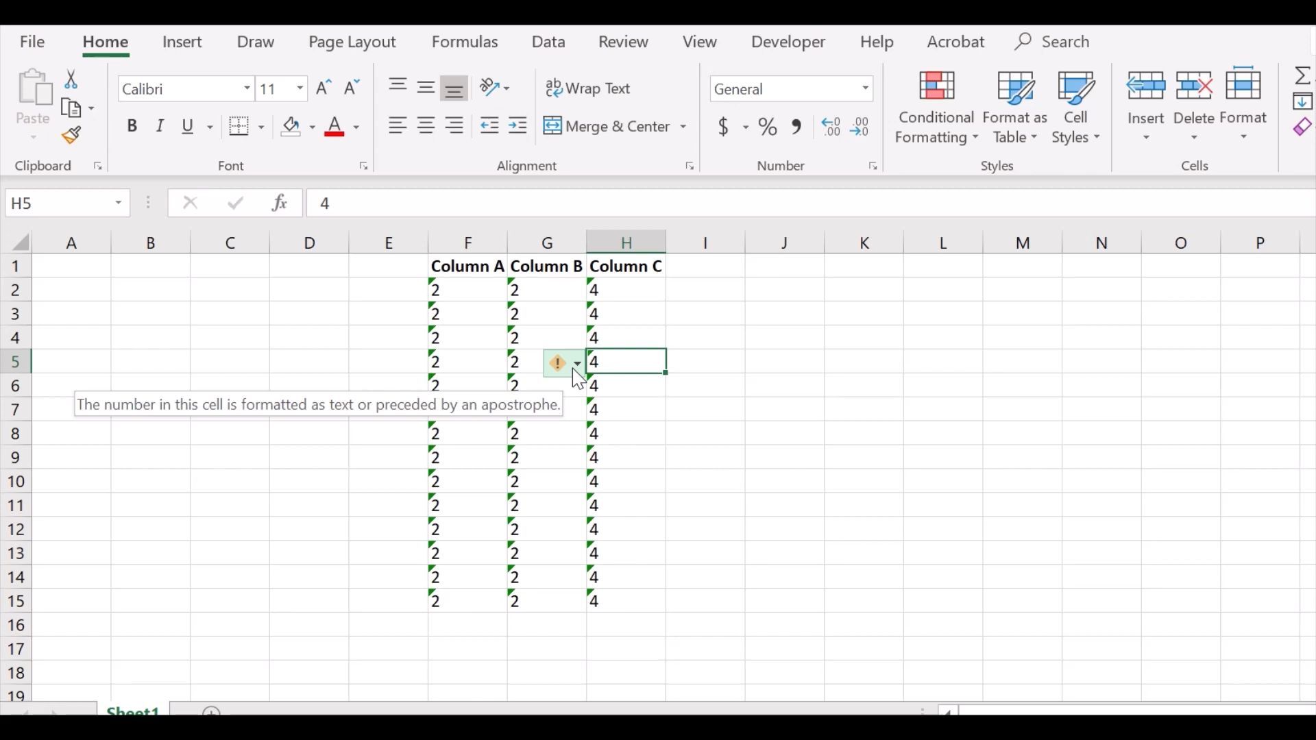
Cells Formatted as Text
If you find yourself in a situation where as soon as you type the formula as hit enter, you see the formula instead of the value, it’s a clear case of the cell being formatted as text.

When a cell is formatted as text, it considers the formula as a text string and shows it as is.
It doesn’t force it to calculate and give the result.
And it has an easy fix.
- Change the format to ‘General’ from ‘Text’ (it’s in Home tab in the Numbers group)
- Go to the cell that has the formula, get into the edit mode (use F2 or double click on the cell) and hit Enter
In case the above steps don’t solve the problem, another thing to check is whether the cell has an apostrophe at the beginning. A lot of people add an apostrophe to convert formulas and numbers to text.
If there is an apostrophe, you can simply remove it.
Text Automatically Getting Converted into Dates
Excel has this bad habit of converting that looks like a date into an actual date. For example, if you enter 1/1, Excel would convert it to 01-Jan of the current year.
In some cases, this may be exactly what you want, and in some cases, this may work against you.
And since Excel stores date and time values as numbers, as soon as you enter 1/1, it converts it into a number representing the January 1 of the current year. In my case, when I do this, it converts it into the number 43831 (for 01-01-2020).
This could mess with your formulas if you’re using these cells as an argument in a formula.
How to fix this?
Again, we don’t want Excel to automatically pick the format for us, so we need to clearly specify the format ourselves.
Below are the steps to change the format to text so that it doesn’t automatically convert text to dates:
- Select the cells/range where you want to change the format
- Click on the Home tab

- In the Number group, click on the Format drop-down
- Click on Text


Now, whenever you enter anything in the selected cells, it would be considered as text, and not changed automatically.
Note: The above steps would only work for data entered after the formatting has been changed. It will not change any text that has been converted to date before you made this formatting change.
Another example where this can be really frustrating is when you enter a text/number that has leading zeros. Excel automatically removes these leading zeros as it considers these useless. For example, if you enter 0001 in a cell, Excel will change it to 1. In case you want to keep these leading zeros, use the steps above.
Hidden Rows/Columns Can Give Unexpected Results
This is not a case of formula giving you the wrong result but of using the wrong formula.
For example, suppose you have a dataset as shown below and I want to get the sum of all the visible cells in column C.

In cell C12, I have used the SUM function to get the total sale value for all these given records.

So far so good!
Now, I apply a filter to the item column to only show the records for Printer sales.

And here is the problem – the formula in cell C12 still shows the same result – i.e., the sum of all the records.
As I said, the formula is not giving the wrong result. In fact, the SUM function is working just fine.
The issue is that we have used the wrong formula here.
SUM function can not account for the filtered data and give you the result for all the cells (hidden or visible). If you only want to get the sum/count/average of visible cells, use SUBTOTAL or AGGREGATE functions.
Key takeaway – Understand the correct use and limitations of a function in Excel.
These are some of the common causes that I have seen where your Excel formulas may not work or give unexpected or wrong results. I am sure there are many more reasons for an Excel formula to not work or update.
In case you know of any other reason (maybe something that irks you often), let me know in the comments section.
Hope you found this tutorial useful!
You may also like the following Excel tutorials:
- How to Lock Formulas in Excel
- How to Copy and Paste Formulas in Excel without Changing Cell References
- Show Formulas in Excel Instead of the Values
- Convert Text to Numbers in Excel
- Convert Date to Text in Excel
- Microsoft Excel Won’t Open; How to Fix it!
- Arrow Keys not Working in Excel | Moving Pages Instead of Cells
- 20 Advanced Excel Functions and Formulas
6 Main Reasons for Excel Formula Not Working (with Solution)
- Reason #1 – Cells Formatted as Text
- Reason #2 – Accidentally Typed the keys CTRL + `
- Reason #3 – Values are Different & Result is Different
- Reason #4 – Don’t Enclose Numbers in Double Quotes
- Reason #5 – Check If Formulas are Enclosed in Double Quotes
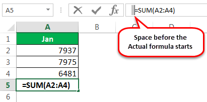
- Reason #6 – Space Before the Excel Formula
Table of contents
- 6 Main Reasons for Excel Formula Not Working (with Solution)
- #1 Cells Formatted as Text
- Solution
- #2 Accidentally Typed the keys CTRL + `
- Solution
- #3 Values are Different & Result is Different
- Solution
- #4 Don’t Enclose Numbers in Double Quotes
- #5 Check If Formulas are Enclosed in Double Quotes
- #6 Space Before the Excel Formula
- Recommended Articles
- #1 Cells Formatted as Text
You are free to use this image on your website, templates, etc, Please provide us with an attribution linkArticle Link to be Hyperlinked
For eg:
Source: Excel Formula Not Working (wallstreetmojo.com)
#1 Cells Formatted as Text
Now let us look at the solutions for the reasons given above for the Excel formula not working.
Now take a look at the first possibility of the formula showing the formula itself, not the result of the formula. For example, look at the below image where the SUM function in excelThe SUM function in excel adds the numerical values in a range of cells. Being categorized under the Math and Trigonometry function, it is entered by typing “=SUM” followed by the values to be summed. The values supplied to the function can be numbers, cell references or ranges.read more shows the formula, not the result.
The first thing we need to look into is the format of the cells; these cells are D1, D2, and D3. So, now take a look at the format of these cells.
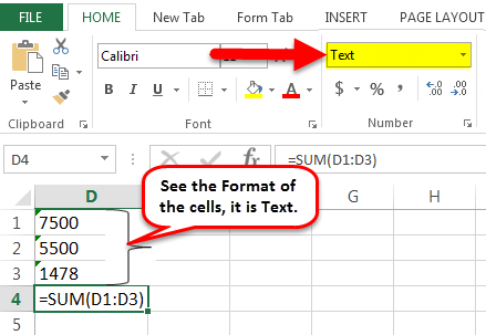
It is formatted as text. When the cells are formatted as text, Excel cannot read numbers and return the result for your applied formula.
Solution
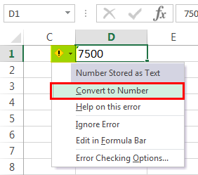
Change the format of the cells to “General” or “Convert to Number.”
- We must first select the cells. Then, on the left-hand side, we can see one small icon. Click on that icon, and choose the option “Convert to Number.”

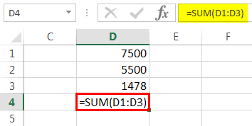
- Now, we must see the result of the formula.

- We are still not getting the result we are looking for. Now, we need to examine whether the formula cell is formatted as text or not.

- Yes, it is formatted as text, so change the cell format to “GENERAL” or “NUMBER.” We must see the result now.


#2 Accidentally Typed the keys CTRL + `
Often in Excel, when working in a hurry, we tend to type keys that are not required, which is an accidental incident. But if we do not know which key we typed, we may get an unusual result.
One such moment is SHOW FORMULAS in excelIn Excel, we can display formulas to investigate the procedure’s relationship. To begin, select the formula tab, then formula auditing, and finally show formulas. In addition, there is a keyboard shortcut for it.read more shortcut key CTRL + `. If we have accidentally typed this key, we may see the result like the picture below.
As we said, the reason could be the accidental pressing of the show formula shortcut key.
Solution
The solution is to try typing the same key again to get back the results of the formula rather than the formula itself.
#3 Values are Different & Result is Different
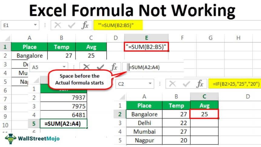
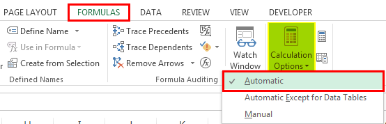
Sometimes, we see different numbers in Excel, but the formula shows different results. For example, the below image displays one such situation.
In cells D1, D2, and D3, we have 10 as the value. In cell D4, we have applied the SUM function to get the total value of cells D1, D2, and D3. But the result says 40 instead of 30.
All the Excel file calculations are set to automatic. But to enhance the speed of the large data files, the user might have changed the auto calculation to a manual one.
Solution
We can fix this in two ways. One is we can turn on the calculation to “Automatic.”
Either we can do one more thing. We can also press the shortcut key F9, which is nothing but “Calculate Now” under the “Formulas” bar.
#4 Don’t Enclose Numbers in Double Quotes
We must pass the numerical values to get the desired result in situations inside the formula. For example, please take a look at the below image; it shows cities and the average temperature in the city.
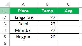
If the temperature is greater than 25, then the average should be 25, and if the temperature is less than 25, then the average should be 20. Finally, we will apply the IF condition in excelIF function in Excel evaluates whether a given condition is met and returns a value depending on whether the result is “true” or “false”. It is a conditional function of Excel, which returns the result based on the fulfillment or non-fulfillment of the given criteria.
read more to get the results.

We have supplied the numerical results double-quotes =IF (B2>25,” 25″,” 20″). Unfortunately, when the numbers are passed in double-quotes, Excel treats them as text values. Therefore, we cannot do any calculations with text numbers.
Always pass the numerical values without double quotes like the below image.
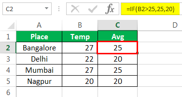
Now, we can do all sorts of calculations with these numerical values.
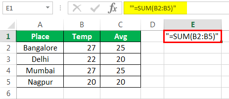
#5 Check If Formulas are Enclosed in Double Quotes
We need to ensure formulas are not wrapped in double quotes. It happens when we copy formulas from online websites and paste them as it is. If the formula is mentioned in double quotes for understanding, we need to remove double quotes and paste them. Otherwise, we may get only the formulas, not the result of the formula.
#6 Space Before the Excel Formula
We all humans make mistakes. Typing mistake is one of the errors for the Excel formula not working. We usually commit day in and day out in our workplace. If we type one or more spaces before we start our formula, it breaks the rule of the formulas in Excel. As a result, we may end up with only the Excel formula, not the result of the formula.
Recommended Articles
This article has been a guide to Excel Formula Not Working and Updating. Here, we discuss the Top 6 reasons and solutions for those Excel formulas not working and updating, practical examples, and a downloadable Excel template. You may learn more about Excel from the following articles: –
- Excel Minus Formula
- Excel VBA IFERROR
- Formula Excel Errors
- Max Formula in Excel
Skip to content
Если существующих функций недостаточно, Excel позволяет добавить новые собственные функции. Мы ранее рассказали, как их создать и как использовать, чтобы ваша работа стала проще. В этой статье мы рассмотрим проблемы, с которыми вы можете столкнуться при использовании созданных пользовательских функций в своих рабочих книгах. Я постараюсь показать вам, что их вызывает и как легко их решить.
Вот о каких проблемах мы поговорим:
- Почему не пересчитывается пользовательская функция?
- Как создать функцию, которая всегда пересчитывается
- Почему пользовательской функции нет в списке?
- Не отображается подсказка
Почему не пересчитывается пользовательская функция?
Excel не пересчитывает автоматически все формулы в рабочей книге или на листе. Если вы изменили какую-то ячейку в таблице, то пересчитываются только формулы, которые на нее ссылаются. Excel знает, что изменить результат могут только ячейки, которые указаны в аргументах формулы. Следовательно, изменения в этих ячейках – единственное, на что Excel обращает внимание при принятии решения о необходимости пересчета.
Это позволяет избежать ненужных вычислений, которые ничего не меняют на вашем рабочем листе.
Это относится и к пользовательским формулам. Excel не может проверить код VBA и определить другие ячейки, которые также могли повлиять на результат.
Поэтому результат вашей формулы может не измениться, когда вы произвели изменения в рабочей книге. И вам будет казаться, что ваша пользовательская функция или макрос не работает.
Чтобы решить эту проблему, вам просто нужно использовать оператор Application.Volatile. Прочтите следующую главу, чтобы получить пошаговые инструкции по его применению.
Как создаются волатильные и не волатильные функции.
По умолчанию пользовательская функция в Excel не волатильная. Это означает, что она пересчитывается только тогда, если значение любой из ячеек, на которые она ссылается, изменится. Но если изменятся формат ячеек, имя рабочего листа, имя файла, то никаких изменений не произойдет.
К примеру, вам необходимо записать в ячейке имя вашей рабочей книги.
Для этого вы создали пользовательскую функцию:
Function WorkbookName() As String
WorkbookName = ThisWorkbook.Name
End Function
Вы записали =WorkbookName() в ячейку и получили там имя файла. Но вот вы решили переименовать файл и сохранили его под другим именем. И вдруг видите, что значение в ячейке не изменилось! Там по-прежнему старое имя файла, которое уже не существует.
Поскольку в этой функции нет аргументов, она не пересчитывается (даже если вы измените имя рабочей книги, закроете ее, а затем снова откроете).
Для пересчета всех формул в файле вам необходимо использовать комбинацию клавиш CTRL+ALT+F9.
Как решить эту проблему, чтобы лишний раз не нажимать клавиши?
Чтобы формула пересчитывалась при каждом изменении на листе, вам потребуется дополнительная строка кода. В начале кода нужно использовать специальный оператор:
Application.Volatile
То есть, ваш код будет выглядеть так:
Function WorkbookName() As String
Application.Volatile
WorkbookName = ThisWorkbook.Name
End Function
Ваша функция стала волатильной. То есть, она будет пересчитана автоматически, если была изменена любая ячейка на рабочем листе или произошло любое другое изменение в рабочей книге. Как только вы, к примеру, переименуете рабочую книгу или лист, эти изменения вы увидите немедленно.
Однако имейте в виду, что слишком много волатильных функций может замедлить работу Excel. Ведь многие формулы выполняют достаточно сложные вычисления и работают с большими диапазонами данных.
Поэтому рекомендую применять волатильность только там, где это действительно необходимо.
Почему пользовательской функции нет в списке?
При вводе первых букв имени пользовательской функции она появляется в выпадающем списке рядом с ячейкой ввода, как и стандартные функции Excel.
Вы можете видеть такой пример на скриншоте ниже.

Однако, это происходит не всегда. Какие ошибки могут стать причиной того, что вы не видите вашу функцию в списке?
Если у вас Excel 2003-2007, то пользовательская функция никогда не появляется в выпадающем списке. Там вы можете увидеть только стандартные функции.
Но даже если вы используете более новую версию Excel, есть еще одна ошибка, которую вы можете случайно сделать.
Пользовательская функция должна находиться в стандартном модуле VBA. Что это означает?
Когда вы добавляете новый модуль для записи кода, автоматически создается папка Modules, в которую записываются все модули. Это вы видите на скриншоте ниже.

Но иногда случается, что новый модуль не был создан.
На скриншоте ниже вы видите, что код находится в таких модулях, как ThisWorkbook или Sheet1.
Нельзя размещать настраиваемую функцию в области кода рабочего листа или рабочей книги. Эту ошибку вы и видите на скриншоте ниже.

В этом случае функция работать не будет. Она также не появится в выпадающем списке. Поэтому код всегда должен находиться в папке Modules, как показано на первом скриншоте.
Не отображается подсказка для пользовательской функции
Еще одна проблема заключается в том, что при вводе пользовательской функции не отображается подсказка. Когда мы используем стандартную функцию, то всегда видим всплывающую подсказку для неё и для её аргументов.
Если у вас много пользовательских функций, то вам будет сложно запомнить, какие вычисления делает каждая из них. Еще труднее будет запоминать, какие аргументы нужно использовать. Думаю, вы хотели бы иметь полное описание для каждого из них.
Для этого я предлагаю дополнительно использовать метод Application.MacroOptions. Он поможет вам показать описание не только функции, но и каждого её аргумента в окне Мастера. Это окно вы видите, когда нажимаете кнопку fx в строке формул.
Давайте попробуем создать такую справку.
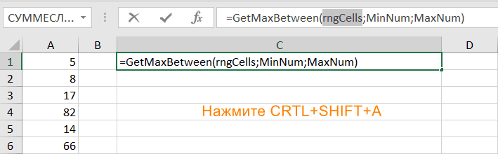
Ранее мы с вами рассматривали настраиваемую функцию GetMaxBetween(). Она находит максимальное число в указанном интервале и использует три аргумента: диапазон числовых значений, а также максимальное и минимальное значение для поиска.
Добавим в нее описание и справочную информацию. Для этого нужно создать и запустить команду Application.MacroOptions.
Для GetMaxBetween вы можете выполнить следующую команду:
Sub RegisterUDF()
Dim strFuncName As String   ' имя функции, которую регистрируем
Dim strDescr As String   'описание для самой функции
Dim strArgs() As String ' описание для аргументов
    'Регистрируем функцию GetMaxBetween
    ReDim strArgs(1 To 3) ' номер аргумента (от 1 до 3)
    strFuncName = "GetMaxBetween"
    strDescr = "Максимальное значение в указанном диапазоне"
    strArgs(1) = "Диапазон ячеек"
    strArgs(2) = "Нижняя граница интервала"
    strArgs(3) = "Верхняя граница интервала"
    Application.MacroOptions Macro:=strFuncName, _
                             Description:=strDescr, _
                             ArgumentDescriptions:=strArgs, _
                             Category:="Определенные пользователем"
End Sub
или
Sub RegisterUDF()
    Application.MacroOptions Macro:="GetMaxBetween", _
        Description:= "Максимальное значение в указанном диапазоне", _
        Category:= "Определенные пользователем", _
        ArgumentDescriptions:=Array( _
            "Диапазон ячеек", _
            "Нижняя граница интервала", _
            "Верхняя граница интервала")
End Sub
Переменная strFuncName — это имя. strDescr —описание. В переменных strArgs записаны подсказки для каждого аргумента.
Вы спросите, для чего нужен четвертый аргумент Application.MacroOptions? Этот необязательный аргумент называется Category и указывает на категорию функций Excel, в которую будет помещена наша пользовательская функция GetMaxBetween(). Вы можете присвоить ему имя любой из существующих категорий: Математические, Статистические, Логические и т.д. Можно указать имя новой категории, в которую вы будете помещать созданные вами макросы. Если же не использовать аргумент Category, то она будет автоматически помещена в раздел «Определенные пользователем».
Вставьте код в окно модуля, как показано на скриншоте ниже:
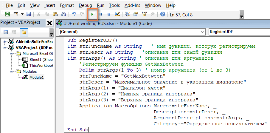
Затем нажмите кнопку “Run”.
Команда выполнит все настройки для использования кнопки fx с вашей функцией GetMaxBetween().
Теперь посмотрим, что у нас получилось. Если попробовать вставить в ячейку функцию при помощи инструмента Вставка функции, то увидите, что GetMaxBetween() находится в категории «Определенные пользователем»:

В качестве альтернативы, вы можете просто начать вводить имя функции в ячейку, как это показано на скриншоте ниже. В выпадающем списке вы увидите свою пользовательскую функцию и можете выбрать ее.

После этого вызовите Мастер при помощи кнопки fx.
Чтобы открыть Мастер функций, вы также можете использовать комбинацию клавиш CTRL + A.

В окне Мастера вы видите описание для функции, а также подсказку для первого аргумента. Если установить курсор на второй или третий аргумент, вы также увидите подсказки для них.
Если вы захотите поменять текст этих подсказок, в коде RegisterUDF() измените значения переменных strDescr и strArgs. Затем снова выполните команду RegisterUDF().
Если вы захотите отменить все сделанные настройки и очистить описание, выполните этот код:
Sub UnregisterUDF()
    Application.MacroOptions Macro:="GetMaxBetween", _
Description:=Empty, ArgumentDescriptions:= Empty, Category:=Empty
End Sub
Есть еще один способ получить подсказку при вводе пользовательской функции.
Введите название функции и затем нажмете комбинацию CTRL+SHIFT+A :
=GetMaxBetween( + CTRL + Shift + A
Вы увидите список всех аргументов функции:
К сожалению, здесь вы не увидите описания функции и её аргументов. Но если названия аргументов достаточно информативны, то это может помочь. Всё же это лучше, чем ничего.
Чтобы создать интеллектуальную подсказку, которая будет работать так же, как в стандартных функциях Excel, необходимо немного больше усилий. К сожалению, Microsoft не предоставляет для этого никаких возможностей.
Единственным доступным решением в настоящее время является Excel-DNA IntelliSense extension. Более подробную информацию вы можете найти по этой ссылке.
Надеюсь, эти рекомендации помогут вам решить проблему, когда ваша пользовательская функция не работает либо работает не так, как вам хотелось бы.
 Сумма по цвету и подсчёт по цвету в Excel — В этой статье вы узнаете, как посчитать ячейки по цвету и получить сумму по цвету ячеек в Excel. Эти решения работают как для окрашенных вручную, так и с условным форматированием. Если…
  Проверка данных с помощью регулярных выражений — В этом руководстве показано, как выполнять проверку данных в Excel с помощью регулярных выражений и пользовательской функции RegexMatch. Когда дело доходит до ограничения пользовательского ввода на листах Excel, проверка данных очень полезна. Хотите… Поиск и замена в Excel с помощью регулярных выражений — В этом руководстве показано, как быстро добавить пользовательскую функцию в свои рабочие книги, чтобы вы могли использовать регулярные выражения для замены текстовых строк в Excel. Когда дело доходит до замены… Как извлечь строку из текста при помощи регулярных выражений — В этом руководстве вы узнаете, как использовать регулярные выражения в Excel для поиска и извлечения части текста, соответствующего заданному шаблону. Microsoft Excel предоставляет ряд функций для извлечения текста из ячеек. Эти функции…
  4 способа отладки пользовательской функции — Как правильно создавать пользовательские функции и где нужно размещать их код, мы подробно рассмотрели ранее в этой статье. Чтобы решить проблемы при создании пользовательской функции, вам скорее всего придется выполнить… Как создать пользовательскую функцию? — В решении многих задач обычные функции Excel не всегда могут помочь. Если существующих функций недостаточно, Excel позволяет добавить новые настраиваемые пользовательские функции (UDF). Они делают вашу работу легче. Мы расскажем,…
Hello,
I have a Dell Inspiron (7000 series 2 in 1) too having Windows 10 installed. I am not often using the shortcuts you mentionned, but I just gave them a try. And I have seen, that they are also not working correctly on this system.
For me, the behaviour is: I opened Excel with a blank workbook and add some worksheets. Then, I created a second blank workbook. If I try to switch from workbook A to workbook B by using Ctrl+Tab, this works fine. Then, I created a third workbook. If I then use Ctrl+Tab, only the last two workbooks are cycled. I can add more workbooks, same behaviour. Only the last two workbooks are cycled.
If I try Ctrl+Shift+Tab, then all 4 workbooks are cycled. So, I think, there is a problem there and something is going wrong. May be an Excel/Office bug, a Windows 10 bug or some drivers affecting this. More people having this problem?
On my desktop computer, all is working fine (same Excel 2016 Version 1703, Build 7967.2030). I did not test other laptops/computers.
Best regards,
Mourad
Bottom Line: Learn about the different calculation modes in Excel and what to do if your formulas are not calculating when you edit dependent cells.
Skill Level: Beginner
Watch the Tutorial
Download the Excel File
You can follow along using the same workbook I use in the video. I’ve attached it below:
Why Aren’t My Formulas Calculating?
If you’ve ever been in a situation where the formulas in your spreadsheet are not automatically calculating as they should, you know how frustrating it can be.
This was happening to my friend Brett. He was telling me that he was working with a file and it wasn’t recalculating the formulas as he was entering data. He found that he had to edit each cell and hit Enter for the formula in the cell to update.
And it was only happening on his computer at home. His work computer was working just fine. This was driving him crazy and wasting a lot of time.
The most likely cause of this issue is the Calculation Option mode, and it’s a critical setting that every Excel user should know about.
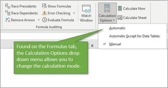
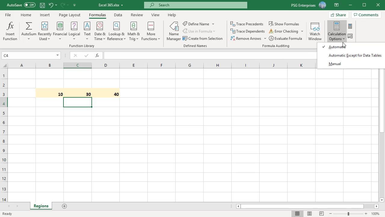
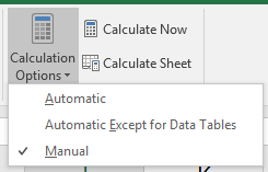
To check what calculation mode Excel is in, go to the Formulas tab, and click on Calculation Options. This will bring up a menu with three choices. The current mode will have a checkmark next to it. In the image below, you can see that Excel is in Manual Calculation Mode.
When Excel is in Manual Calculation mode, the formulas in your worksheet will not calculate automatically. You can quickly and easily fix your problem by changing the mode to Automatic. There are cases when you might want to use Manual Calc mode, and I explain more about that below.
Calculation Settings are Confusing!
It’s really important to know how the calculation mode can change. Technically, it’s is an application-level setting. That means that the setting will apply to all workbooks you have open on your computer.
As I mention in the video above, this was the issue with my friend Brett. Excel was in Manual calculation mode on his home computer and his files weren’t calculating. When he opened the same files on his work computer, they were calculating just fine because Excel was in Automatic calculation mode on that computer.
However, there is one major nuance here. The workbook (Excel file) also stores the last saved calculation setting and can change/override the application-level setting.
This should only happen for the first file you open during an Excel session.
For example, if you change Excel to manual calc mode before you save & close the file, then that setting is stored with the workbook. If you then open that workbook as the first workbook in your Excel session, the calculation mode will be changed to manual.
All subsequent workbooks that you open during that session will also be in manual calculation mode. If you save and close those files, the manual calc mode will be stored with the files as well.
The confusing part about this behavior is that it only happens for the first file you open in a session. Once you close the Excel application completely and then re-open it, Excel will return to automatic calculation mode if you start by opening a new blank file or any file that is in automatic calculation mode.
Therefore, the calculation mode of the first file you open in an Excel session dictates the calculation mode for all files opened in that session. If you change the calculation mode in one file, it will be changed for all open files.
Note: I misspoke about this in the video when I said that the calculation setting doesn’t travel with the workbook, and I will update the video.
The 3 Calculation Options
There are three calculation options in Excel.
Automatic Calculation means that Excel will recalculate all dependent formulas when a cell value or formula is changed.
Manual Calculation means that Excel will only recalculate when you force it to. This can be with a button press or keyboard shortcut. You can also recalculate a single cell by editing the cell and pressing Enter.
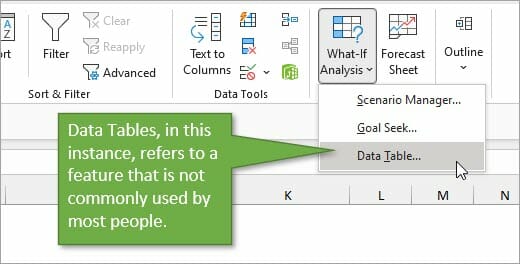
Automatic Except for Data Tables means that Excel will recalculate automatically for all cells except those that are used in Data Tables. This is not referring to normal Excel Tables that you might work with frequently. This refers to a scenario-analysis tool that not many people use. You find it on the Data tab, under the What-If Scenarios button. So unless you’re working with those Data Tables, it’s unlikely you will ever purposely change the setting to that option.
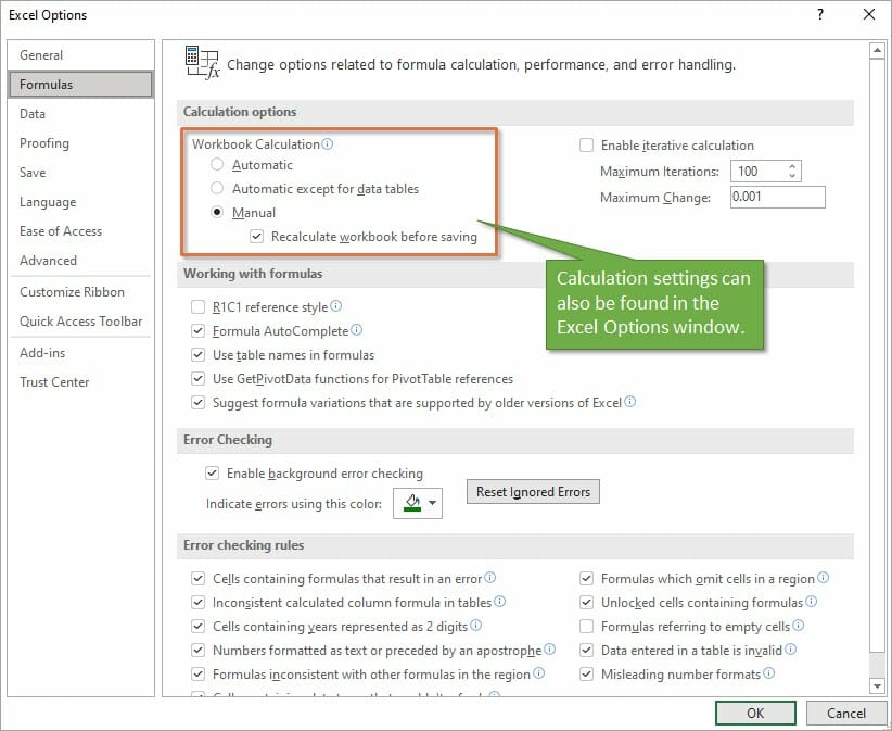
In addition to finding the Calculation setting on the Data tab, you can also find it on the Excel Options menu. Go to File, then Options, then Formulas to see the same setting options in the Excel Options window.
Under the Manual Option, you’ll see a checkbox for recalculating the workbook before saving, which is the default setting. That’s a good thing because you want your data to calculate correctly before you save the file and share it with your co-workers.
Why Would I Use Manual Calculation Mode?
If you are wondering why anyone would ever want to change the calculation from Automatic to Manual, there’s one major reason. When working with large files that are slow to calculate, the constant recalculation whenever changes are made can sometimes slow your system. Therefore people will sometimes switch to Manual mode while working through changes on worksheets that have a lot of data, and then will switch back.
When you are in Manual Calculation mode, you can force a calculation at any time using the Calculate Now button on the Formulas tab.
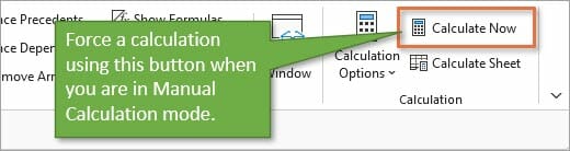
The keyboard shortcut for Calculate Now is F9, and it will calculate the entire workbook. If you want to calculate just the current worksheet, you can choose the button below it: Calculate Sheet. The keyboard shortcut for that choice is Shift + F9.
Here is a list of all Recalculate keyboard shortcuts:
| Shortcut | Description |
| F9 | Recalculate formulas that have changed since the last calculation, and formulas dependent on them, in all open workbooks. If a workbook is set for automatic recalculation, you do not need to press F9 for recalculation. |
| Shift+F9 | Recalculate formulas that have changed since the last calculation, and formulas dependent on them, in the active worksheet. |
| Ctrl+Alt+F9 | Recalculate all formulas in all open workbooks, regardless of whether they have changed since the last recalculation. |
| Ctrl+Shift+Alt+F9 | Check dependent formulas, and then recalculate all formulas in all open workbooks, regardless of whether they have changed since the last recalculation. |
Macro Changing to Manual Calculation Mode
If you find that your workbook is not automatically calculating, but you didn’t purposely change the mode, another reason that it may have changed is because of a macro.
Now I want to preface this by saying that the issue is NOT caused by all macros. It’s a specific line of code that a developer might use to help the macro run faster.
The following line of VBA code tells Excel to change to Manual Calculation mode.
Application.Calculation = xlCalculationManual
Sometimes the author of the macro will add that line at the beginning so that Excel does not attempt to calculate while the macro runs. The setting should then changed be changed back at the end of the macro with the following line.
Application.Calculation = xlCalculationAutomatic
This technique can work well for large workbooks that are slow to calculate.
However, the problem arises when the macro doesn’t get to finish—perhaps due to an error, program crash, or unexpected system issue. The macro changes the setting to Manual and it doesn’t get changed back.
As I mention in the video, this was exactly what happened to my friend Brett, and he was NOT aware of it. He was left in manual calc mode and didn’t know why, or how to get Excel calculating again.
Therefore, if you are using this technique with your macros, I encourage you to think about ways to mitigate this issue. And also warn your users of the potential of Excel being left in manual calc mode.
I also recommend NOT changing the Calculation property with code unless you absolutely need to. This will help prevent frustration and errors for the users of your macros.
Conclusion
I hope this information is helpful for you, especially if you are currently dealing with this particular issue. If you have any questions or comments about calculation modes, please share them in the comments.
Why are my functions not working in Excel?
Cause: The cell is formatted as Text, which causes Excel to ignore any formulas. This could be directly due to the Text format, or is particularly common when importing data from a CSV or Notepad file. However, the formulas still won’t start working until you force Excel to reconsider the content.
How do I stop excel debugging?
How to Disable Debug in VBA in Excel
- Go to File, Options and then Customize Ribbon.
- Return to the Excel workbook or worksheet.
- In the Visual Basic editor window, click Tools then VBAProject Properties.
- Click the Protection tab.
- Save the workbook, then close and reopen it for the changes to take effect.
What does debug mean in Excel?
What is VBA’s Debugging Environment? In Excel 2013, VBA’s debugging environment allows the programmer to momentarily suspend the execution of VBA code so that the following debug tasks can be done: Check the value of a variable in its current state. Enter VBA code in the Immediate window to view the results.
How do I enable debugging in Excel?
MS Excel 2016: Debug Mode in VBA
- Check the value of a variable in its current state.
- Enter VBA code in the Immediate window to view the results.
- Execute each line of code one at a time.
- Continue execution of the code.
- Halt execution of the code.
What is Wend in VBA?
WEND statement is used to create a WHILE loop in VBA. You use a WHILE loop when you are not sure how many times you want to execute the VBA code within the loop body. With a WHILE loop, the loop body may not execute even once. WEND statement is a built-in function in Excel that is categorized as a Logical Function.
How does the close statement differ from the Quit statement in VBA?
End Sub can’t be called in the same way Exit Sub can be, because the compiler doesn’t allow it. Immediately exits the Sub procedure in which it appears. Execution continues with the statement following the statement that called the Sub procedure. Exit Sub can be used only inside a Sub procedure.
Does Excel VBA do until?
The Do Until loop is a useful tool in Excel VBA used to repeat a set of steps until the statement is FALSE. When the statement is FALSE we want the loop to stop and the loop naturally comes to an end. So in phrasing the loop the condition is set at the end of the loop.
Microsoft Excel has been one of the most valuable tools since the dawn of modern computing. Over a million people use Microsoft Excel spreadsheets daily to manage projects, track finances, create charts and graphs, and even manage time.
Unlike other applications such as Word, the spreadsheet software uses mathematical formulas and data in cells to calculate values.
However, there are instances when the Excel formulas do not function properly. This article will help you fix problems with Excel formulas.
1. Calculation Options Set to Manual
If you can’t update the value you’ve entered, and it returns the same as you entered, Excel’s calculation option may be set to manual and not automatic.
To fix this, change the calculation mode from Manual to Automatic.
- Open the spreadsheet you’re having trouble with.
- Then from the ribbon, navigate to the Formulas tab, then choose Calculation.
- Select Calculation Options and choose Automatic from the dropdown.
Alternatively, you can adjust the calculation options from Excel options.
Choose the Office button at the top left corner > Excel options > Formulas > Workbook Calculation > Automatic. If you often switch between these two modes, you can create a custom keyboard shortcut for Excel to speed up your work.
2. Cell Is Formatted as Text
You might have accidentally formatted the cells containing the formulas as text. Unfortunately, Excel skips the applied formula when set to text format and displays the plain result instead.
The best way to check for formatting is to click on the cell and check the Number group from the Home tab. If it displays «Text,» click on that and choose General. To recalculate the formula, double-click the cell and press Enter on your keyboard.
3. Show Formulas Button Is Turned On
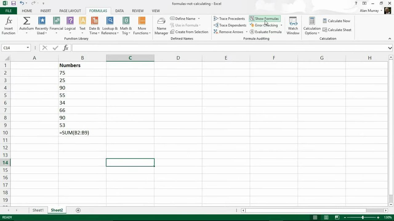
People commonly misuse the Show Formulas button by accidentally turning it on. With this turned on, the applied formulas will not work. You can find this setting under the Formulas tab.
The Show Formulas button is designed for auditing formulas, displaying the formula instead of the result when pressed. This might be a good tool if you want to better understand Excel formulas, but it stops them from working. In this case, turning it off may help resolve the issue.
Go to the Formulas tab > Formula Auditing Group and click the Show Formulas button.
4. Check Your Excel Formula

Even if you’re using an Excel function for beginners, a missing or an extra character might be why your Excel formula isn’t working. For example, when you enter an additional equal to (‘=’) or apostrophe (‘) in a spreadsheet cell, calculations are not performed, causing problems for users. The issue typically occurs when users try to copy a formula from the web.
However, it is simple to fix this problem. Just head over to the cell, select it, and remove the apostrophe or space at the beginning of the formula.
The same goes for the formula’s parentheses. When writing a lengthy formula, make sure you match all parentheses, so the calculations take place in the correct order. Excel helps you by showing parentheses pairs in different colors, so you can easily follow them.
Excel will display an error message when there’s a missing or extra parenthesis.
5. Use Proper Characters to Separate Arguments
You might have to separate function arguments to get the desired outcome depending on which Excel formulas you’re using. You should generally separate arguments using commas, but this may vary depending on your Regional Settings.
For example, in North American countries, you must enter commas to separate arguments, while in Europe, the right character is set to a semicolon. If you’ve used the wrong separating character, Excel might show the «We found a problem with this formula» error. You can try both options and check which one works for you.
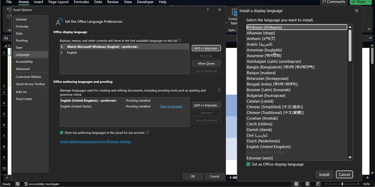
If you’re used to using commas instead of semicolons, or vice versa, you can edit Excel settings to avoid repeating the same error.
- Open Excel’s File menu and go to More > Options.
- From the left pane, select Language.
- In the Office display language section, click the Add a language button.
- Select the wanted language to install and click Install.
- Select it again and click Set as Preferred.
- Test if Excel formulas are now working.
To sync Office settings across your devices when logging in with your Microsoft account, check the Store my authoring languages in the cloud for my account option.
6. Force Excel to Recalculate
Excel allows users to recalculate formulas manually if they prefer not to use automatic calculation settings. You can do this with these methods:
For recalculating an entire spreadsheet, press F9 on your keyboard or choose Calculate Now under Formula Tab. Alternatively, you can recalculate an active sheet by pressing Shift + F9 on your keyboard or selecting Calculate Sheet from the Calculation group under Formula Tab.
You could also recalculate all formulas across all worksheets by pressing the Ctrl + Alt + F9 keyboard combination. Moreover, if you prefer recalculating just one formula from a sheet, select the cell and press Enter.
7. Check for Circular References
Excel formulas might show the wrong results if it uses circular referencing, which refers to the same cell where it does the calculations. Most of the time, Excel will notify you about a circular reference, but it might not do it every time.
Fortunately, you can manually check for this type of reference if you keep getting wrong results out of Excel formulas.
Open the Formulas tab, go to Formula Auditing, and select Error Checking > Circular References. Excel will show which cells have added a circular reference to the formula.
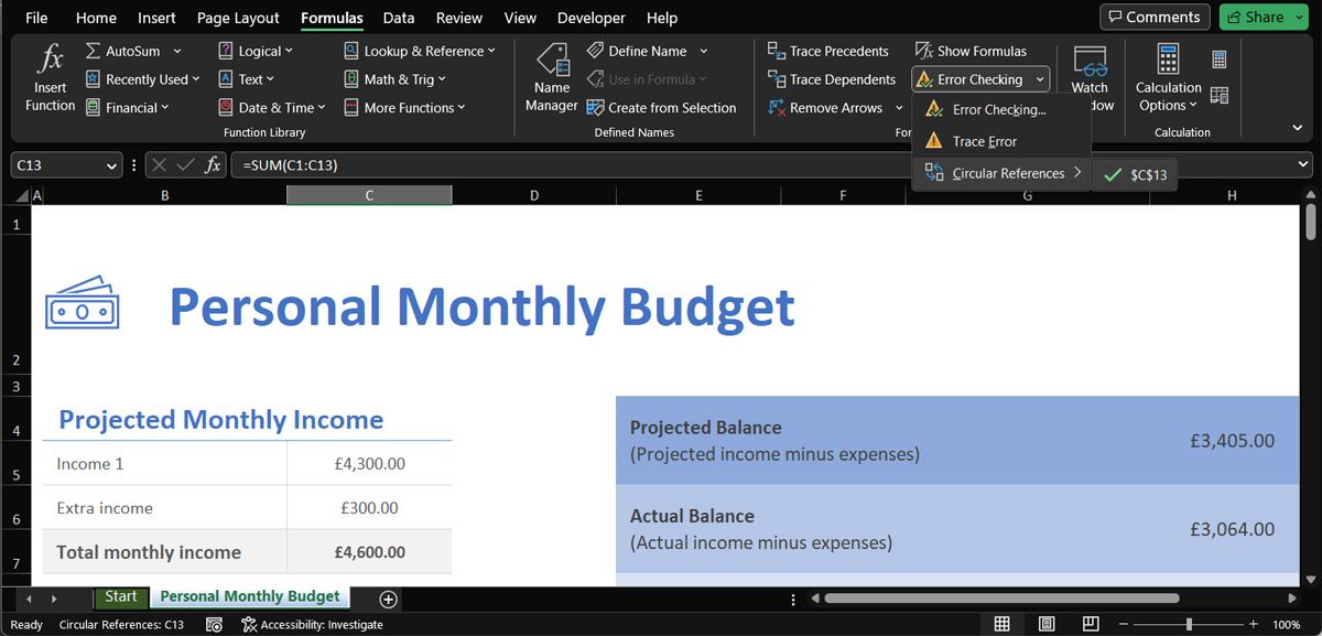
Go to the indicated cells and edit the formula so it doesn’t include the cell showing the results. For example, if the C13 cell shows the result for =SUM(C1:C13), change C13 to C12 within the formula to fix it.
Solve Your Excel Issues With These Fixes
The truth is, there’s not much room for error when writing an Excel formula. A missing parenthesis or the wrong cell format is enough to stop Excel formulas from working as intended.
However, you should know how to fix the issue as you’ll save a lot of time having Excel do the calculations for you.
Author: Oscar Cronquist Article last updated on September 29, 2022
This article explains why your formula is not working properly, there are usually four different things that can go wrong.
Table of Contents
- Formula not working — check arguments
- Formula not working — Number stored as text
- How to change the «manual calculation» setting
- Formula not working — the cell shows the formula and not the result
- Formula not working — formula cell formatted as text
- Formula not working — #NAME! error
- How to troubleshoot a formula not working as intended
1. Formula not working — check the function arguments

This example shows a function in cell B2 that returns a #VALUE! error, this may happen when there is something wrong with the arguments.
The SUBTOTAL function allows you to use a number between 1 and 11, the first argument is in this example 12 which is an invalid argument.
How to quickly show function arguments?
Type the function in a cell, and then the beginning parentheses, Excel instantly shows the arguments and in some cases, allowed values.

Here is a list of Excel functions and their arguments: Excel functions
Here is a list of common errors: Excel formula errors
Back to top
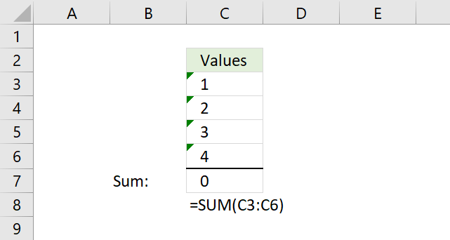
2. How to solve «numbers stored as text»?
The first one is numbers stored as text, demonstrated in the picture above.
Why is the SUM function in cell C7 returning 0 (zero) in the picture above?
The numbers in cell range C3:C6 are stored as text. You can see that by the green arrow in each cell’s top left corner.
Why is this happening?
The cell range C3:C6 was formatted as text cells before you entered the numbers in these cells.
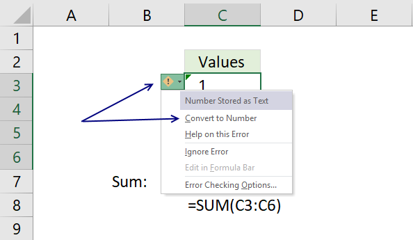
How to solve it?
Select cell range C3:C6, and press with left mouse button on the exclamation mark symbol (or exclamation point if you are American) to open a menu.
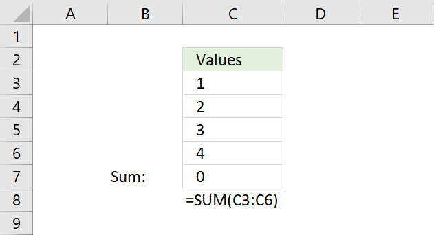
Press with mouse on «Convert to Number», the green arrows disappear and the SUM function formula works as expected again.
Back to top
3. How to change the «manual calculation» setting
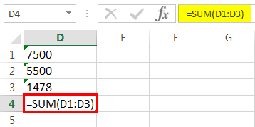
The SUM formula in cell C7 returns 0 (zero), why is this happening?
Check if your workbook is in manual calculation mode. Go to tab «Formulas» on the ribbon, then press with left mouse button on the «Calculations Options» button.
In this case, the setting was on «Manual», changing it back to «Automatic» makes the SUM formula work as intended again.
Back to top
4. The cell shows the formula and not the result — here is how to fix it
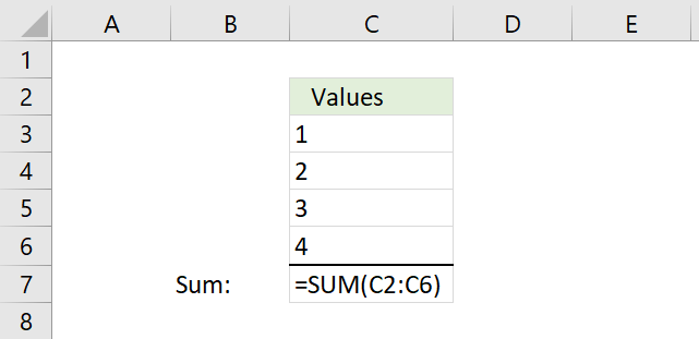
Cell C7 displays the formula, not the result. Why is this happening?
Go to tab «Formulas», check if «Show Formulas» button is enabled (highlighted).
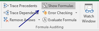
Press with mouse on the «Show Formulas» button to disable it. The cell now shows the result of the SUM calculation. If this is not working, read section 5 below.
Back to top
5. Formula cell formatted as text
The cell in C7 shows the formula? I don’t want that, I want to see the calculation result.
Select cell C7, press CTRL + 1 on your keyboard.
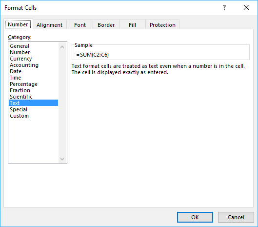
This reveals that the cell is formatted as «Text» making it show the formula and not the result. Press with mouse on «General» and then on the OK button.
Now it shows the output from the formula.
Back to top
6. Formula not working — #NAME? error

The #NAME? error hints that you misspelled the function name.

Tip! Check the suggestions while typing the formula. Use the arrow up and down keys to change the selected suggestion. Use the TAB key to auto-complete the selected suggestion.
Back to top
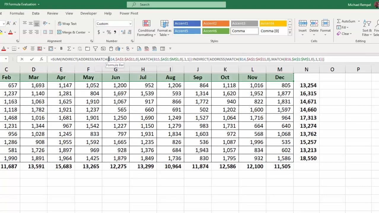
7. How to troubleshoot a formula not working as intended?

The image above shows a formula in cell C6 that returns no error, however, the calculation is wrong. How do we troubleshoot this formula to find what is wrong in the calculation?
The «Evaluate formula» tool lets us see the calculation steps in greater detail. Here is how to start the tool:
- Select the cell you want to troubleshoot, in this example cell C6.
- Go to the tab «Formulas» on the ribbon.
- Press with left mouse button on the «Evaluate Formula» button located on the ribbon.

- A dialog box appears.


The dialog box shows the formula in the white box and has four buttons below. The underlined expression shows what part of the formula will be calculated in the next step.
The italicized text is the most recent result, press with left mouse button on the «Evaluate» button to start the formula evaluation.

Keep press with left mouse button oning on the «Evaluate» button until greyed out to see all steps in the calculation, this helps to identify where the problem is.
The tool shows that the formula multiples values in cells C2 and C3 before adding the number in cell C4. We need to add C2 with C4 and then multiply with C3.
Press with left mouse button on the «Close» button to dismiss the dialog box.
The parentheses allow us to control the order of operation. Here is the final formula:
=(C2+C4)*C3

Back to top
![]()
Find empty cells and sum cells above
This article demonstrates how to find empty cells and populate them automatically with a formula that adds numbers above and […]
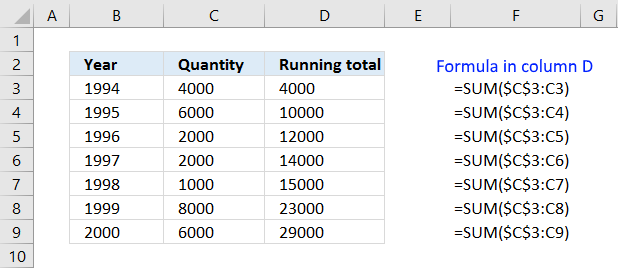
How to create running totals
This article demonstrates a formula that calculates a running total. A running total is a sum that adds new numbers […]
How to sum a cell range
I will in this article demonstrate different ways to sum values, the first method is so easy and fast it’s […]
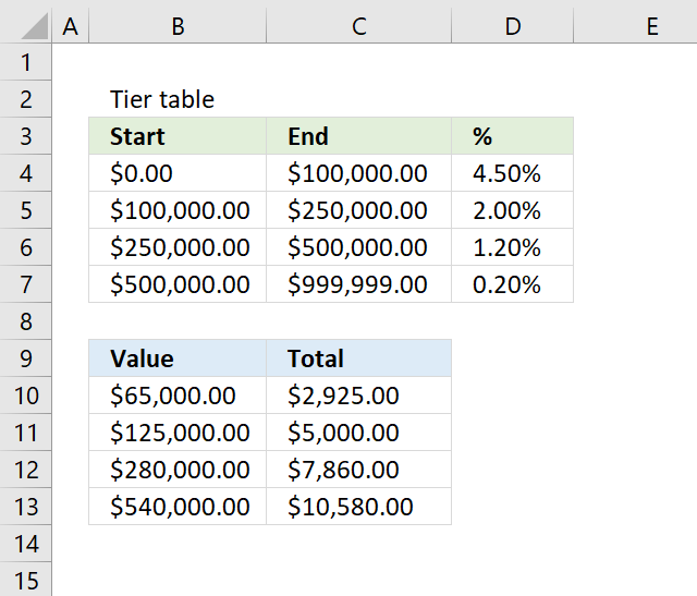
Running totals based on criteria
Andrew asks: LOVE this example, my issue/need is, I need to add the results. So instead of States and Names, […]
Sum based on OR – AND logic
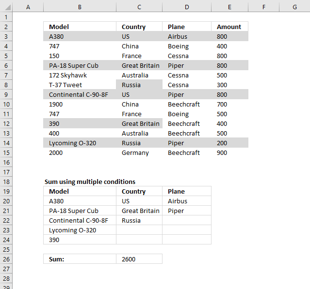
Question: It’s easy to sum a list by multiple criteria, you just use array formula a la: =SUM((column_plane=TRUE)*(column_countries=»USA»)*(column_producer=»Boeing»)*(column_to_sum)) But all […]
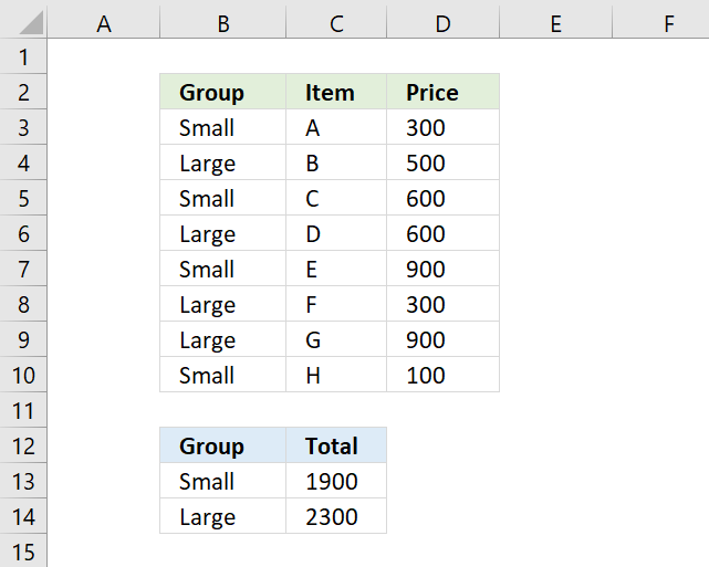
Sum by group
To extract groups from cell range B3:B10 I use the following regular formula in cell B13.
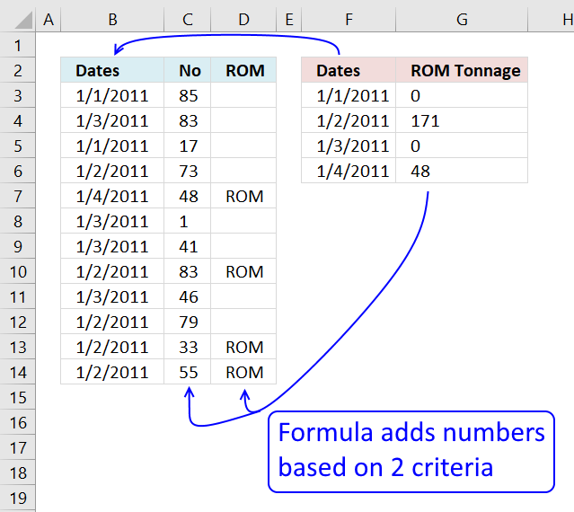
Sum cells based on criteria
Katie asks: I have 57 sheets many of which are linked together by formulas, I need to get numbers from […]
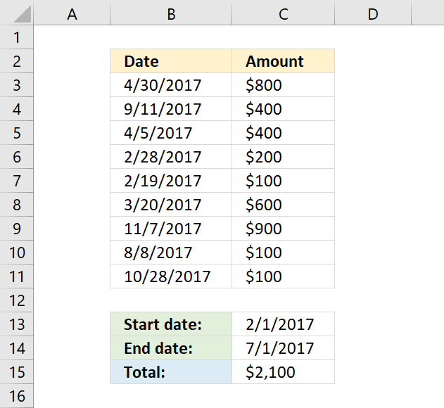
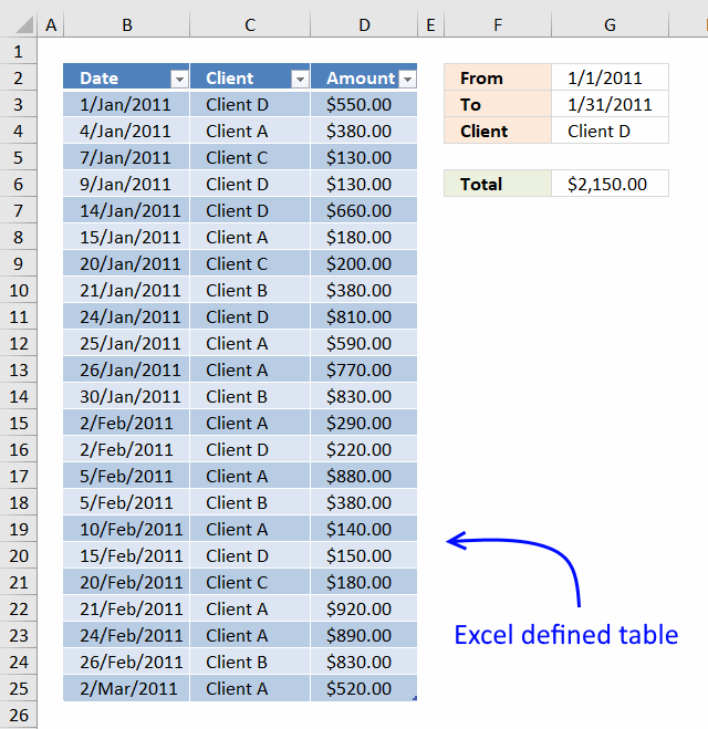
Sum numbers between two dates
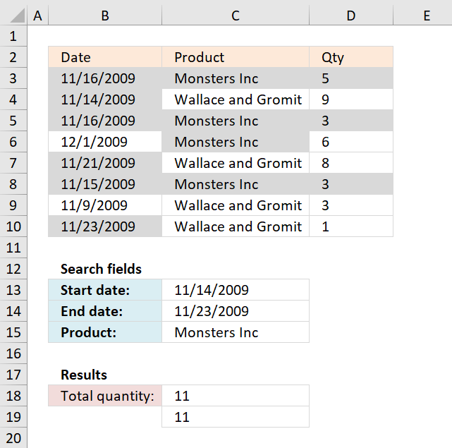
The formula in cell C15 uses two dates two to filter and then sum values in column C, the SUMIFS […]
Sum only visible cells
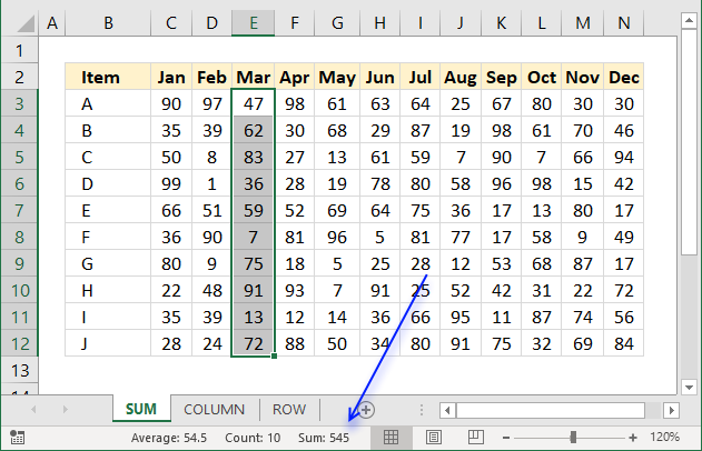
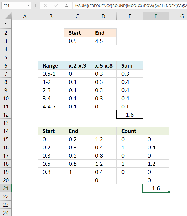
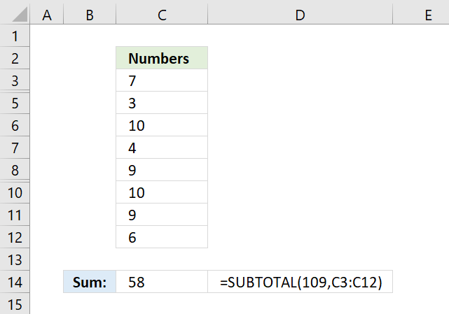
The SUBTOTAL function lets you sum values in a cell range that have some rows hidden or filtered, the picture […]
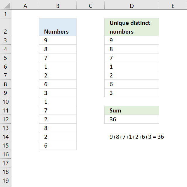
Sum unique distinct numbers
The image above shows numbers in column B, some of these numbers are duplicates. The formula in D12 adds unique […]
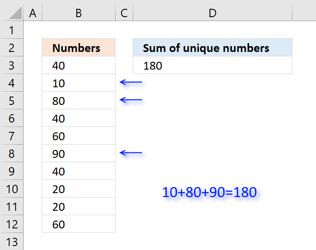
Sum unique numbers
Table of Contents Sum unique numbers Get Excel *.xlsx file Sum unique distinct numbers Get Excel *.xlsx file Sum number […]
Latest updated articles.
More than 300 Excel functions with detailed information including syntax, arguments, return values, and examples for most of the functions used in Excel formulas.
More than 1300 formulas organized in subcategories.
Excel Tables simplifies your work with data, adding or removing data, filtering, totals, sorting, enhance readability using cell formatting, cell references, formulas, and more.
Allows you to filter data based on selected value , a given text, or other criteria. It also lets you filter existing data or move filtered values to a new location.
Lets you control what a user can type into a cell. It allows you to specifiy conditions and show a custom message if entered data is not valid.
Lets the user work more efficiently by showing a list that the user can select a value from. This lets you control what is shown in the list and is faster than typing into a cell.
Lets you name one or more cells, this makes it easier to find cells using the Name box, read and understand formulas containing names instead of cell references.
The Excel Solver is a free add-in that uses objective cells, constraints based on formulas on a worksheet to perform what-if analysis and other decision problems like permutations and combinations.
An Excel feature that lets you visualize data in a graph.
Format cells or cell values based a condition or criteria, there a multiple built-in Conditional Formatting tools you can use or use a custom-made conditional formatting formula.
Lets you quickly summarize vast amounts of data in a very user-friendly way. This powerful Excel feature lets you then analyze, organize and categorize important data efficiently.
VBA stands for Visual Basic for Applications and is a computer programming language developed by Microsoft, it allows you to automate time-consuming tasks and create custom functions.
A program or subroutine built in VBA that anyone can create. Use the macro-recorder to quickly create your own VBA macros.
UDF stands for User Defined Functions and is custom built functions anyone can create.
A list of all published articles.