
For beginners, it would sometimes be confusing to understand the terminologies used in Excel. An Active Cell by appearance is not a tricky phrase; however, it can be confusing at times. An active cell, often known as a current cell, cell pointer, or selected cell that appears as a rectangular box that displays the cell in a sheet.
With an active cell, you can find on which cell you are working and what data is entered. A cell in the sheet can carry multiple kinds of data along with formulas or different data formatting that helps in automatic analysis. With data formatting, you can tell an active cell what kind of data you can choose such as fractions, currency, percentages, and dates.
How to Find an Active Cell in a Selection?
It does not matter how many cells you have selected, there would be just one active cell on the sheet. You can find an active cell in two different ways:
Visual Identifier of Active Cell
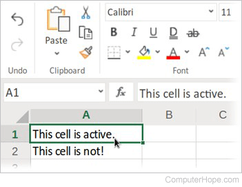
While selecting a range of cells, you will see one cell is different in color than others. For instance, here you can see A1:D10 cells are selected and other cells are presented in a dark grey color, cell A1 is in a light shade color.

It clearly shows that this is an active cell that appears with a different color. For more understanding, start typing anything and it will appear in the active cell.
Where is the Content of the Active Cell?
Do you know where the formula bar is on the screen?
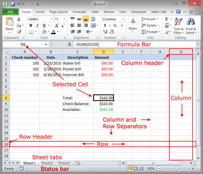
The content of an active cell generally appears in the formula bar. Here in this example, the formula bar has a formula in cell D8. In the formula, “=SUM(D2:D5)”, you can add the values of cell D2 to D5 in order to calculate the total value, which is $162.00.
The cell and formula bar displays the formula when you choose D8.
How to Change the Active Cell with Shortcut?
With a mouse or keyboard, you can move around the sheet quickly to change the active cell. If you need to quickly reach another cell, place your cursor on that cell directly:
- In the Name Box, put the cell reference of the targeted cell.
- For instance, suppose you need to be in cell Z100, simply type Z100 in the Name Box and press ENTER.
- You would instantly go to that cell within microseconds.

Summary:
So, now you have come to know what is an active cell in Excel and how you can change it quickly. Hopefully, the above-mentioned information is useful to you and helps you find an answer to your query. A combination of cells mutually makes rows and columns that ultimately become an Excel Spreadsheet.
The basis of an Excel sheet starts from a cell, that’s why you need to understand it thoroughly.
As discusssed in previous lessons, Excel Columns are represented by Column letters and Rows are represented by Row numbers. Each cell in Excel worksheet is identified by a combination of a Column Letter and a row number.
The Active cell inside Excel Worksheet is used to identify the cell which is currently active. The thick border gridlines around the cell indicates that it is the Active cell inside Excel Worksheet. The Active cell is where the focus is on and where the data will be entered when a key is typed on keyboard. Below image shows the Actice Cell as C5, which is hi-lighted with a thick border.
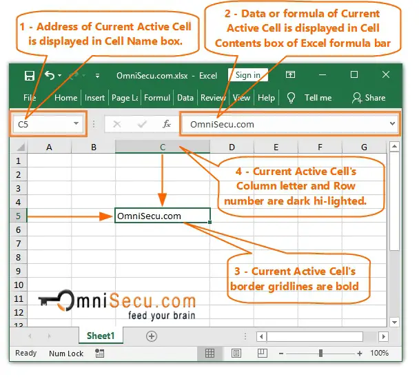
The current Active Cell in above image of worksheet is C5. The current Active Cell can be identified as below.
1 — Address of Current Active Cell is displayed in Cell Name box.
2 — Data or Formula of Current Active Cell can be viewed inside Cell Contents box of Excel Formula bar.
3 — Current Active Cell’s border gridlines are bold.
4 — Current Active Cell’s Column letter and Row number are dark highlighted.
Updated: 10/07/2019 by
Alternatively called a cell pointer, current cell, or selected cell, an active cell is a rectangular box that highlights the cell in a spreadsheet. An active cell helps identify what cell is being worked with and where data will be entered.
Active cell overview
In the picture below of Microsoft Excel, you can see that the active cell is D8 and is shown in the top-left corner.
Tip
When you first start Excel the active cell is the first cell, which is always A1. You can move the cell pointer by pressing the arrow keys or Enter on your keyboard, or you can click any cell using your computer mouse. If you’re using the keyboard, you can also press the F2 to edit the active cell.
How is an active cell identified?
An active cell or selected cell can be identified many ways. First, as shown in the picture above of Microsoft Excel, the active cell has a bold black box around the cell. Also, the column and row are highlighted. In our example picture, the column header «D» and row header «8» are highlighted in yellow. The active cell is also shown in the top-left portion of the window (Name box), which is «D8» in our example.
Where is the content of the active cell is displayed?
The content of the active cell is shown in the formula bar. In the screenshot above, the formula bar displays the formula in cell D8. The formula, «=SUM(D2:D5)», adds the values of cells D2 through D5 to compute their total value, $162.00. When cell D8 is selected, both the cell and the formula bar display the formula. When any other cell is selected, cell D8 shows the result of its formula, the total $162.00.
How do you change the active cell?
You can change the active cell by clicking any other cell with your left mouse button or with the arrow keys on your keyboard to move the selected cell. If the cell contains no data, you can begin typing to insert new data into that cell. If the cell already contains data, you can click up on the formula bar to change that data or press the F2 on the keyboard.
Which cell is active when Excel is first opened?
When you open a new Excel spreadsheet for the first time, the first cell is selected by default, which is A1 (the first cell of row A and column one). If you’ve worked on an Excel spreadsheet in the past, the active cell is the last active cell position. For example, if you last left the spreadsheet on cell C65, when it is saved and re-opened, it should return to cell C65.
Absolute cell reference, Active, Cell, Name box, Spreadsheet terms
Содержание
- Working with the Active Cell
- Moving the Active Cell
- Selecting the Cells Surrounding the Active Cell
- Support and feedback
- Active cell
- Active cell overview
- How is an active cell identified?
- Where is the content of the active cell is displayed?
- How do you change the active cell?
- Which cell is active when Excel is first opened?
- Работа с активной ячейкой
- Перемещение активной ячейки
- Выделение ячеек вокруг активной ячейки
- Поддержка и обратная связь
- VBA Active Cell
- Active Cell in Excel VBA
- #1 – Referencing in Excel VBA
- #2 – Active Cell Address, Value, Row, and Column Number
- #3 – Parameters of Active Cell in Excel VBA
- Recommended Articles
- Using Active Cell in VBA in Excel (Examples)
- What is an Active Cell in Excel?
- Using Active Cell in VBA in Excel
- Active Cell Properties and Methods
- Making a Cell the Active Cell
- Clear the Active Cell
- Get the Value from the Active Cell
- Formating the Active Cell (Color, Border)
- Offsetting From the Active Cell
- Get ActiveCell Row or Column Number
- Assign Active Cell Value to a Variable
- Select a Range of Cells Starting from the Active Cell
Working with the Active Cell
The ActiveCell property returns a Range object that represents the cell that is active. You can apply any of the properties or methods of a Range object to the active cell, as in the following example. While one or more worksheet cells may be selected, only one of the cells in the selection can be the ActiveCell.
Note You can work with the active cell only when the worksheet that it is on is the active sheet.
Moving the Active Cell
Use the Range .Activate method to designate which cell is the active cell. For example, the following procedure makes B5 the active cell and then formats it as bold.
Note To select a range of cells, use the Select method. To make a single cell the active cell, use the Activate method.
Use the Offset property to move the active cell. The following procedure inserts text into the active cell in the selected range and then moves the active cell one cell to the right without changing the selection.
Selecting the Cells Surrounding the Active Cell
The CurrentRegion property returns a range or ‘island’ of cells bounded by blank rows and columns. In the following example, the selection is expanded to include the cells that contain data immediately adjoining the active cell. This range is then formatted with the Currency style.
Support and feedback
Have questions or feedback about Office VBA or this documentation? Please see Office VBA support and feedback for guidance about the ways you can receive support and provide feedback.
Источник
Active cell
Alternatively called a cell pointer, current cell, or selected cell, an active cell is a rectangular box that highlights the cell in a spreadsheet. An active cell helps identify what cell is being worked with and where data will be entered.
Active cell overview
In the picture below of Microsoft Excel, you can see that the active cell is D8 and is shown in the top-left corner.
When you first start Excel the active cell is the first cell, which is always A1. You can move the cell pointer by pressing the arrow keys or Enter on your keyboard, or you can click any cell using your computer mouse. If you’re using the keyboard, you can also press the F2 to edit the active cell.
How is an active cell identified?
An active cell or selected cell can be identified many ways. First, as shown in the picture above of Microsoft Excel, the active cell has a bold black box around the cell. Also, the column and row are highlighted. In our example picture, the column header «D» and row header «8» are highlighted in yellow. The active cell is also shown in the top-left portion of the window (Name box), which is «D8» in our example.
Where is the content of the active cell is displayed?
The content of the active cell is shown in the formula bar. In the screenshot above, the formula bar displays the formula in cell D8. The formula, «=SUM(D2:D5)», adds the values of cells D2 through D5 to compute their total value, $162.00. When cell D8 is selected, both the cell and the formula bar display the formula. When any other cell is selected, cell D8 shows the result of its formula, the total $162.00.
How do you change the active cell?
You can change the active cell by clicking any other cell with your left mouse button or with the arrow keys on your keyboard to move the selected cell. If the cell contains no data, you can begin typing to insert new data into that cell. If the cell already contains data, you can click up on the formula bar to change that data or press the F2 on the keyboard.
Which cell is active when Excel is first opened?
When you open a new Excel spreadsheet for the first time, the first cell is selected by default, which is A1 (the first cell of row A and column one). If you’ve worked on an Excel spreadsheet in the past, the active cell is the last active cell position. For example, if you last left the spreadsheet on cell C65, when it is saved and re-opened, it should return to cell C65.
Источник
Работа с активной ячейкой
Свойство ActiveCell возвращает объект Range, представляющий активную ячейку. К активной ячейке можно применить любое свойство или метод объекта Range, как показано в следующем примере. Хотя можно выделить одну или несколько ячеек листа, в выделенном фрагменте только к одной ячейке можно применить свойство ActiveCell.
Примечание Работать с активной ячейкой можно только в том случае, если лист, на который она находится, является активным листом.
Перемещение активной ячейки
Чтобы указать, какая ячейка является активной, используйте метод Range .Activate. Например, в следующей процедуре ячейка B5 назначается активной с последующим ее форматированием полужирным шрифтом.
Примечание Чтобы выбрать диапазон ячеек, используйте метод Select . Чтобы сделать одну ячейку активной, используйте метод Activate.
Для перемещения активной ячейки используйте свойство Offset. Следующая процедура вставляет текст в активную ячейку в выбранном диапазоне, а затем перемещает активную ячейку вправо на одну ячейку, не изменяя выделенный фрагмент.
Выделение ячеек вокруг активной ячейки
Свойство CurrentRegion возвращает диапазон или «остров» ячеек, ограниченный пустыми строками и столбцами. В следующем примере выделенный фрагмент расширяется для включения ячеек, содержащих данные, непосредственно примыкающие к активной ячейке. Затем этот диапазон форматируется с использованием денежного стиля.
Поддержка и обратная связь
Есть вопросы или отзывы, касающиеся Office VBA или этой статьи? Руководство по другим способам получения поддержки и отправки отзывов см. в статье Поддержка Office VBA и обратная связь.
Источник
VBA Active Cell


Active Cell in Excel VBA
The active cell is the currently selected cell in a worksheet. The active cell in VBA can be used as a reference to move to another cell or change the properties of the same active cell or the cell reference provided by the active cell. We can access an active cell in VBA by using the application.property method with the keyword active cell.
In Excel, there are millions of cells, and you are unsure which one is an active cell. For example, look at the below image.

In the above pic, we have many cells. Finding which one is an active cell is very simple; whichever cell is selected. It is called an “active cell” in VBA.
Look at the name box Name Box In Excel, the name box is located on the left side of the window and is used to give a name to a table or a cell. The name is usually the row character followed by the column number, such as cell A1. read more if your active cell is not visible in your window. It will show you the active cell address. For example, in the above image, the active cell address is B3.
Even when many cells are selected as a range of cells, whatever the first cell is in, the selection becomes the active cell. For example, look at the below image.

Table of contents
#1 – Referencing in Excel VBA
For example, if we want to select cell A1 and insert the value “Hello,” we can write it in two ways. Below is the way of selecting the cell and inserting the value using the VBA “RANGE” object
Code:

It will first select the cell A1 “Range(“A1″). Select”
Then, it will insert the value “Hello” in cell A1 Range(“A1”).Value = “Hello”
Now, we will remove the line Range(“A1”). Value = “Hello” and use the active cell property to insert the value.
Code:

Similarly, first, it will select the cell A1 “Range(“A1”). Select.“
But here, we have used ActiveCell.Value = “Hello” instead of Range(“A1”).Value = “Hello”
We have used the active cell property because the moment we select cell A1 it becomes an active cell. So, we can use the Excel VBA active cell property to insert the value.
#2 – Active Cell Address, Value, Row, and Column Number
Let’s show the active cell’s address in the message box to understand it better. Now, look at the below image.

In the above image, the active cell is “B3,” and the value is 55. So, let us write code in VBA to get the active cell’s address.
Code:

Run this code using the F5 key or manually. Then, it will show the active cell’s address in a message box.
Output:

Similarly, the below code will show the value of the active cell.
Code:

Output:

The below code will show the row number of the active cell.
Code:

Output:

The below code will show the column number of the active cell.
Code:

Output:

#3 – Parameters of Active Cell in Excel VBA
The active cell property has parameters as well. After entering the property, the active cell opens parenthesis to see the parameters.

Using this parameter, we can refer to another cell as well.
For example, ActiveCell (1,1) means whichever cell is active. If you want to move down one row to the bottom, you can use ActiveCell (2,1). Here 2 does not mean moving down two rows but rather just one row down. Similarly, if you want to move one column to the right, then this is the code ActiveCell (2,2)
Look at the below image.

In the above image, the active cell is A2. To insert value to the active cell, you write this code.
Code:

Run this code manually or through the F5 key. It will insert the value “Hiiii” into the cell.

If you want to insert the same value to the below cell, you can use this code.
Code:

It will insert the value to the cell below the active cell.

You can use this code if you want to insert the value to one column right then.
Code:

It will insert “Hiiii” to the next column cell of the active cell.

Like this, we can reference the cells in VBA using the active cell property.
We hope you have enjoyed it. Thanks for your time with us.
You can download the VBA Active Cell Excel Template here:- VBA Active Cell Template
Recommended Articles
This article has been a guide to VBA Active Cell. Here, we learned the concept of an active cell to find the address of a cell. Also, we learned the parameters of the active cell in Excel VBA along with practical examples and a downloadable template. Below you can find some useful Excel VBA articles: –
Источник
Using Active Cell in VBA in Excel (Examples)
‘Active Cell’ is an important concept in Excel.
While you don’t have to care about the active cell when you’re working on the worksheet, it’s an important thing to know when working with VBA in Excel.
Proper use of the active cell in Excel VBA can help you write better code.
In this tutorial, I first explained what is an active cell, and then show you some examples of how to use an active cell in VBA in Excel.
This Tutorial Covers:
What is an Active Cell in Excel?
An active cell, as the name suggests, is the currently active cell that will be used when you enter any text or formula in Excel.
For example, if I select cell B5, then B5 becomes my active cell in the worksheet. Now if I type anything from my keyboard, it would be entered in this cell, because this is the active cell.
While this may sound obvious, here is something not that obvious – when you select a range of cells, even then you would only have one active cell.
For example, if I select A1:B10, although I have 20 selected cells, I still have only one single active cell.
So now, if I start typing any text or formula, it would only be entered in the active cell.
You can identify the active cell by looking at the difference in color between the active cell in all the other cells in the selection. You would notice that the active cell is of a lighter shade than the other selected cells.

Another quick way to know which cell is the active cell is by looking at the Name box (the field that is next to the formula bar). The cell reference of the active cell would be shown in the Name Box.

Using Active Cell in VBA in Excel
Now that I’ve explained what is an active cell in a worksheet in excel, let’s learn how an Active cell can be used in Excel VBA.
Active Cell Properties and Methods
In VBA, you can use an active cell in two ways:
- To get the information about it (these are called Properties)
- To perform some action on it (these are called Methods)
Here is how you can access all the properties and methods of an active cell in VBA:
- Open a Module in Excel VBA editor
- Type the phrase ‘ActiveCell’
- Enter a dot (.) after the word ActiveCell
As soon as you do this, you would notice that a set of properties and methods appear as a drop-down (this is called an IntelliSense in Excel VBA).
In the drop-down that appears, you would see two types of options – the one that has a green icon and the one that has a gray icon (with a hand).
The one with the grey icons is the Properties, and the one with the green icons is the Methods.
Some examples of Methods would include Activate, AddComment, Cut, Delete, Clear, etc. As you can notice, these are actions that can be performed on the active cell.
Some examples of Properties would include Address, Font, HasFormula, Interior.Color. All these are properties of the active cell that gives you information about that active cell.
For example, you can use this to get the cell address of the active cell or change the interior cell color of the cell.
Now let’s have a few simple VBA code examples that you can use in your day-to-day work when working with active cell in excel
Making a Cell the Active Cell
To make any cell the active cell, you first have to make sure that it is selected.
If you only have one single cell selected, it by default becomes the active cell.
Below is the VBA code to make cell B5 the active cell:
In the above VBA code, I have first specified the cell address of the cell that I want to activate (which is B5), and then I use the activate method to make it the active cell.
When you only want to make one single cell the active cell, you can also use the select method (code below):
As I mentioned earlier, you can only have one active cell even if you have a range of cell selected.
With VBA, you can first select a range of cells, and then make any one of those cells the active cell.
Below the VBA code that would first select range A1:B10, and then make cell A5 the active cell:
Clear the Active Cell
Below is the VBA code that would first make cell A5 the active cell, and then clear its content (cell content as well any formatting applied to the cell).
Note that I have shown you the above code just to show you how the clear method work with active cell. In VBA, you don’t need to always select or activate the cell to perform any method on it.
For example, you can also clear the content of cell A5 using the below code:
Get the Value from the Active Cell
Below the VBA code that could show you a message box displaying the value in the active cell:
Similarly, you can also use a simple VBA code to show the cell address of the active cell (code below):
The above code would show the address in absolute reference (such as $A$5).

Formating the Active Cell (Color, Border)
Below the VBA code that would make the active cell blue in color and change the font color to white.
Note that I have used the inbuilt color constant (vbBlue and vbWhite). You can also use the RGB constant. For example, instead of vbRed, you can use RGB(255, 0, 0)
Offsetting From the Active Cell
VBA in Excel allows you to refer to cells relative to the position of the active cell (this is called offsetting).
For example, if my active cell is cell A1, I can use the offset property on the active cell and refer to the cell below it by specifying the position of that row corresponding to the active cell.
Let me show you an example.
The above code first activate cell A1 and makes it the active cell. It then uses the offset property on the active cell, to refer to the cell which is one row below it.
And in the same line in the code, I have also assigned a value “Test” to that cell which is one row below the active cell.
Let me show you another example where offsetting from the active cell could be used in a practical scenario.
Below I have a VBA code that first activates cell A1, and then uses the offset property to cover 10 cells below the active cell and enter numbers from 1 to 10 in cell A1:A10.
The above code uses a For Next loop that runs 10 times (and each time the value of the variable ‘i’ increases by 1). And since I am also using ‘i’ in the offset property, it keeps going one cell down with each iteration.
Get ActiveCell Row or Column Number
Below the VBA code that will show you the row number of the active cell in message box:
And the below code will show you the column number in a message box:
Assign Active Cell Value to a Variable
You can also use VBA to assign the active cell to a variable. Once this is done, you can use this variable instead of the active cell in your code.
And how does this help? Good Question!
When you assign the active cell to a variable, you can continue to use this variable instead of the active cell. The benefit here is that unlike the active cell (which can change when other sheets or workbooks are activated) your variable would continue to refer to the original active cell it was assigned to.
So if you are writing a VBA code that cycles through each worksheet and activates these worksheets, while your active cell would change as new sheets are activated, the variable to which you assigned the active cell initially wouldn’t change.
Below is an example code that defines a variable ‘varcell’ and assigns the active cell to this variable.
Select a Range of Cells Starting from the Active Cell
And the final thing I want to show you about using active cell in Excel VBA is to select an entire range of cells starting from the active cell.
A practical use case of this could be when you want to quickly format a set of cells in every sheet in your workbook.
Below is the VBA code that would select cells in 10 rows and 10 columns starting from the active cell:
When we specify two cell references inside the Range property, VBA refers to the entire range covered between there two references.
For example, Range(Range(“A1”), Range(“A10”)).Select would select cell A1:A10.
Similarly, I have used it with active cell, Where the first reference is the active cell itself, and the second reference offsets the active cell by 10 rows and 10 columns.
I hope this tutorial has been useful for you in understanding how active cell works in Excel VBA.
Other Excel tutorials you may also find useful:
Источник
A lot of new Excel users often get confused with the terminologies used in Excel.
One such term that you would often find in many of the Excel tutorials and videos is the Active Cell.
If you do not know what an active cell in Excel is, I’m going to tell you everything about it in this short tutorial.
It’s really simple but very useful to know when working with Excel.
An Excel worksheet is made up of individual cells – the small rectangle box where you enter data.
When you select one of these cells, that becomes the active cell.
For example, if I select cell A1 using my mouse or my keyboard, then it would become the active cell in that Excel worksheet.

So if I enter any formula or any text, it would be entered in the active cell.
When you have only selected one single cell in a worksheet, by default that is the active cell.
But what if you select more than one cell? What if I select a range of cells (say A1:D10)?
Even if you have a range of cells selected you would still have only one single active cell in that Excel file.
Note that everything that I cover in this article is applicable for both Excel as well as Google Sheets (and even other similar spreadsheet tools).
How to Identify the Active Cell in a Selection?
As I already mentioned, if you select a range of cells (say A1:D10), Despite the fact that you have multiple cells selected, there would still only be one active cell.
There are two easy ways to quickly identify which cell is the active cell:
Visual Identifier of Active Cell
When you select a range of cells, you would notice that one cell has a different color than the rest of the selection.
For example, below I have selected cells A1:D10, and you can see that while all the other cells are in dark gray color, cell A1 has a lighter shade color.

This is an indication that this cell (which has a different color than the rest of the selection) is the active cell.
At this point, if you start typing anything, that would be entered in the active cell.
Active Cell Reference in the Name Box
Another super quick way to identify which cell is the active cell is by looking at the Name Box (which is on the left of the formula bar).
The cell reference of the active cell would be visible in the Name Box.

So if you select one single cell, that cell is the active cell and its reference would be shown in the Name Box.
And in case you select multiple cells, since only one of those cells could be the active cell, you can simply have a look at the name box, and see its cell reference there.
Shortcut to Change the Active Cell
While you can use your mouse or your keyboard to quickly move around in the worksheet and change the active cell, in case you want to quickly take your cursor to a far-off cell and make that one the active cell, here’s a cool trick.
Enter the cell reference (of the cell where you want to quickly go) in the Name Box.
For example, if I want to quickly go to cell Z100, I would type Z100 in the Name Box and hit Enter, and it would instantly take me there

Formatting the Active Cell
When you select one single cell in Excel, it becomes the active cell and you can apply any formatting or changes to that specific cell.
And when you select a range of cells, although only one cell would be the active cell, any formatting changes that you apply to that selection would be applied to all the cells (and not just the active cell).
So remember this – when you have a range of cells selected, when you type anything, it would be entered only in the active cell. But if you apply any formatting changes (such as changing the color, border, or cell format), it would be applied to the entire selection.
Some Advanced Active Cell Tricks
Now that you have a good understanding of what is an active cell in Excel, let me also show you a couple of simple tricks that are often used by advanced Excel users.
Enter Formula in All the Selected Cells
When you select a range of cells, and you enter any text or formula, it has only entered in the active cell.
But in many cases, you would want that same text or that same formula to be entered in the entire selection.
For example, below I have a data set where I have Names in column A comma and I want to enter their Departments in column B.

So remember this – when you have a range of cells selected, when you type anything, it would be entered only in the active cell. But if you apply any formatting changes (such as changing the color, border, or cell format), it would be applied to the entire selection.
In this example, I want to enter the same department (say ‘Sales’) in all these cells.
Instead of doing it 1 by 1, or entering it in one cell and then copy-pasting it in other cells, let me show you a faster way.
- Select the cells in which you want to enter the data

- Enter the data (which would automatically be entered in the active cell)

- Hold the Control key and press the Enter key

And Voila!!!!
The same text has been entered for all the cells in the selection.
Similarly, you can also do the same thing with formulas. enter the formula in the active cell, then hold the Control key and hit the Enter key and the formula would be entered in all the selected cells.
And a great thing about entering formulas this way is that it would automatically adjust the cell reference.
A practical example of this would be when you have a dataset with blank cells and you want to fill blank cells with 0 or some text such as NA or a dash. You can select all the blank cells (using the Go To Special technique) and then fill all the blank cells in one go.
Data Entry in a Specific Sequence
This is a less-known Excel trick that could be quite useful if you have a data entry job.
When you select a single cell in Excel, enter the data or formula in that cell, and then hit the enter key, you would automatically be taken to the cell below it.
And here comes the trick.
When you select a range of cells, and then you enter any text or formula, it would be entered in the active cell.
And now when you hit the enter key, you would be taken to the next cell in the selection itself. So if the next cell in this election is below the active cell, you would be taken there, else you would be taken to the next cell in the selection.
For example, if I select cells A1, B2, C3, and D4 (as shown below), enter some text in the active cell (which is cell A1), and then hit the enter key, I would automatically be taken to cell B2 (and not A2).

Once I enter the data in cell B2 and hit the enter key, I would automatically be taken to cell C3 and so on.
Using Active Cell Property in VBA
If you write VBA macro codes, having a good understanding of how the active cell works would be quite useful.
In Excel VBA programming, you can use the active cell as a point of reference and then write a code around it.
Let me give you an example.
Suppose I want to quickly enter the serial numbers from 1 to 10 (starting from the active cell), and also apply some formatting (make the cell color yellow and apply a border to it)
Below is the VBA code that would do this for me.
Sub Formatting()
For i = 1 To 10
    With ActiveCell.Offset(i - 1, 0)
        .Interior.Color = vbYellow
        .Borders.LineStyle = xlContinuous
        .Borders.Weight = xlThin
        .Value = i
    End With
Next i
End Sub
This VBA code works by using the active cell as the anchor and then covering 10 cells below it. in each of these cells, a serial number is entered and the formatting is applied.
Since this VBA code is dependent on the active cell, whenever I select a cell (thereby making it the active cell) and run this VBA code, it would start from that cell and format the 10 cells below it.
While this is a very simple example, the existence of the concept of the active cell actually makes programming quite easy in Excel.
What Happens to the Active Cell When You Activate Some Other Sheet or Workbook?
As I mentioned, there could only be one active cell. No matter which worksheet/workbook is activated, there would only be one active cell.
When you move away from the current worksheet and activate another worksheet (say you are in Sheet1 and then you go to Sheet2), your active cell would now be in the currently active worksheet (which would be Sheet2).
The same happens with Excel workbooks. If you activate another Excel workbook, then your active cell would be in that activated workbook.
And then if you switch back to your earlier workbook, your active cell would then be in the earlier book.
I hope now you are all clear about the concept of the active cell and how it can be used in Excel and VBA.
I hope you found this Excel tutorial useful.
Other Excel tutorials you may also like:
- SetFocus in Excel VBA – How to Use it?
- How to Set the Default Font in Excel (Windows and Mac)
- How to Press Enter in Excel and Stay in the Same Cell?
- How to Compare Two Cells in Excel? (Exact/Partial Match)
- How to Flash an Excel Cell (Easy Step-by-Step Method)
- Edit Cell in Excel (Keyboard Shortcut)
- What Does F2 Do in Excel?