Ms excel value of logical expression 23 74 - Word и Excel - помощь в работе с программами

Show that in:

(
The average value of sin⁡mxcos⁡nxsin m x cos n x (over a period)

=12π∫−ππsin⁡mxcos⁡nxdx=0.=frac{1}{2 pi} int_{-pi}^pi sin m x cos n x d x=0 .

The average value of sin⁡mxsin⁡nxsin m x sin n x (over a period)

=12π∫−ππsin⁡mxsin⁡nxdx={0,m≠n,12,m=n≠0,0,m=n=0.=frac{1}{2 pi} int_{-pi}^pi sin m x sin n x d x= begin{cases}0, & m neq n, \ frac{1}{2}, & m=n neq 0, \ 0, & m=n=0 .end{cases}

The average value of cos⁡mxcos⁡nxcos m x cos n x (over a period)

=12π∫−ππcos⁡mxcos⁡nxdx={0,m≠n,12,m=n≠01,m=n=0.=frac{1}{2 pi} int_{-pi}^pi cos m x cos n x d x= begin{cases}0, & m neq n, \ frac{1}{2}, & m=n neq 0 \ 1, & m=n=0 .end{cases}

)
the average values (over a period) of sin⁡mxsin⁡nxsin m x sin n x and of cos⁡mxcos⁡nxcos m x cos n x (m≠n)(m neq n) are zero, by using the complex exponential forms for the sines and cosines as in (∫−ππsin⁡mxcos⁡nxdx=∫−ππeimx−e−imx2i⋅einx+e−inx2dxint_{-pi}^pi sin m x cos n x d x=int_{-pi}^pi frac{e^{i m x}-e^{-i m x}}{2 i} cdot frac{e^{i n x}+e^{-i n x}}{2} d x)

Источник

What is IF Function in Excel?

IF function in Excel evaluates whether a given condition is met and returns a value depending on whether the result is “true” or “false”. It is a conditional function of Excel, which returns the result based on the fulfillment or non-fulfillment of the given criteria.

For example, the IF formula in Excel can be applied as follows:

“=IF(condition A,“value B”,“value C”)”

The IF excel function returns “value B” if condition A is met and returns “value C” if condition A is not met.

It is often used to make logical interpretations which help in decision-making.

What is IF Function in Excel?
- Syntax of the IF Excel Function
- How to Use IF Function in Excel?
  - Example #1
  - Example #2
  - Example #3
  - Example #4
  - Example #5
- Guidelines for the Multiple IF Statements
- Frequently Asked Question
- IF Excel Function Video
- Recommended Articles

Syntax of the IF Excel Function

The syntax of the IF function is shown in the following image:

The IF excel function accepts the following arguments:

Logical_test: It refers to the condition to be evaluated. The condition can be a value or a logical expression.
Value_if_true: It is the value returned as a result when the condition is “true”.
Value_if_false: It is the value returned as a result when the condition is “false”.

In the formula, the “logical_test” is a required argument, whereas the “value_if_true” and “value_if_false” are optional arguments.

The IF formula uses logical operators to evaluate the values in a range of cells. The following table shows the different logical operatorsLogical operators in excel are also known as the comparison operators and they are used to compare two or more values, the return output given by these operators are either true or false, we get true value when the conditions match the criteria and false as a result when the conditions do not match the criteria.read more and their meaning.

Operator	Meaning
=	Equal to
>	Greater than
>=	Greater than or equal to
<	Less than
<=	Less than or equal to
<>	Not equal to

How to Use IF Function in Excel?

Let us understand the working of the IF function with the help of the following examples in Excel.

You can download this IF Function Excel Template here – IF Function Excel Template

Example #1

If there is no oxygen on a planet, life is impossible. If oxygen is available on a planet, then life is possible. The following table shows a list of planets in column A and the information on the availability of oxygen in column B. We have to find the planets where life is possible, based on the condition of oxygen availability.

Let us apply the IF formula to cell C2 to find out whether life is possible on the planets listed in the table.

The IF formula is stated as follows:

“=IF(B2=“Yes”, “Life is Possible”, “Life is Not Possible”)

The succeeding image shows the IF formula applied to cell C2.

The subsequent image shows how the IF formula is applied to the range of cells C2:C5.

Drag the cells to view the output of all the planets.

The output in the below worksheet shows life is possible on the planet Earth.

Flow Chart of Generic IF Excel Function

The IF Function Flow Chart for Mars (Example #1)

The flow of IF function flowchart for Jupiter and Venus is the same as the IF function flowchart for Mars (Example #1).

The IF Function Flow Chart for Earth

Hence, the IF excel function allows making logical comparisons between values. The modus operandi of the IF function is stated as: If something is true, then do something; otherwise, do something else.

Example #2

The following table shows a list of years. We want to find out if the given year is a leap year or not.

A leap year has 366 days; the extra day is the 29th of February. The criteria for a leap year are stated as follows:

The year will be exactly divisible by 4 and not exactly be divisible by 100 or
The year will be exactly divisible by 400.

In this example, we will use the IF function along with the AND, OR, and MOD functions to find the leap years.

We use the MOD function to find a remainder after a dividend is divided by a divisor.

The AND functionThe AND function in Excel is classified as a logical function; it returns TRUE if the specified conditions are met, otherwise it returns FALSE.read more evaluates both the conditions of the leap years for the value “true”. The OR functionThe OR function in Excel is used to test various conditions, allowing you to compare two values or statements in Excel. If at least one of the arguments or conditions evaluates to TRUE, it will return TRUE. Similarly, if all of the arguments or conditions are FALSE, it will return FASLE.read more evaluates either of the condition for the value “true”.

We will apply the MOD function to the conditions as follows:

If MOD(year,4)=0 and MOD(year,100)<>(is not equal to) 0, then the year is a leap year.

If MOD(year,400)=0, then the year is a leap year; otherwise, the year is not a leap year.

The IF formula is stated as follows:

“=IF(OR(AND((MOD(year,4)=0),(MOD(year,100)<>0)),(MOD(year,400)=0)),“Leap Year”, “Not A Leap Year”)”

The argument “year” refers to a reference value.

The following images show the output of the IF formula applied in the range of cells.

The following image shows how the IF formula is applied to the range of cells B2:B18.

The succeeding table shows the years 1960, 2028, and 2148 as leap years and the remaining as non-leap years.

The result of the IF excel formula is displayed for the range of cells B2:B18 in the following image.

Example #3

The succeeding table shows a list of drivers and the directions they undertook to reach the destination. It is preceded by an image of the road intersection explaining the turns taken by the drivers and their destinations. The right turn leads to town B, and the left turn leads to town C. Identify the driver’s destination to town B and town C.

Road Intersection Image

Let us apply the IF excel function to find the destination. Here, the condition is mentioned as follows:

If the driver turns right, he/she reaches town B.
If the driver turns left, he/she reaches town C.

We use the following IF formula to find the destination:

“=IF(B2=“Left”, “Town C”, “Town B”)”

The succeeding image shows the output of the IF formula applied to cell C2.

Drag the cells to use the formula in the range C2:C11. Finally, we get the destinations of each driver for their turning movements.

The below image displays the IF formula applied to the range.

The output of the IF formula and the destinations are displayed in the succeeding image.

The result shows that six drivers reached town C, and the remaining four have reached town B.

Example #4

The following table shows a list of items and their inventory levels. We want to check if the specific item is available in the inventory or not using the IF function.

Let us list the name of items in column A and the number of items in column B. The list of data to be validated for the entire items list is shown in the cell E2 of the below image.

We use the Excel IF along with the VLOOKUP functionThe VLOOKUP excel function searches for a particular value and returns a corresponding match based on a unique identifier. A unique identifier is uniquely associated with all the records of the database. For instance, employee ID, student roll number, customer contact number, seller email address, etc., are unique identifiers.
read more to check the availability of the items in the inventory.

The VLOOKUP function looks up the values referring to the number of items, and the IF function will check whether the item number is greater than zero or not.

We will apply the following IF formula in the F2 cell:

“=IF(VLOOKUP(E2,A2:B11,2,0)=0, “Item Not Available”,“Item Available”)”

If the lookup value of an item is equal to 0, then the item is not available; else, the item is available.

The succeeding image shows the result of the IF formula in the cell F2.

Select “bat” in the E2 item cell to know whether the item is available or not in the inventory (as shown in the following image).

Example #5

The following table shows the list of students and their marks. The grade criteria are provided based on the marks obtained by the students. We want to find the grade of each student in the list.

We apply the Nested IF in Excel since we have multiple criteria to find and decide each student’s grade.

The Nesting of IF function uses the IF function inside another IF formula when multiple conditions are to be fulfilled.

The syntax of Nesting of IF function is stated as follows:

“=IF( condition1, value_if_true1, IF( condition2, value_if_true2, value_if_false2 ))”

The succeeding table represents the range of scores and the grades, respectively.

Let us apply the multiple IF conditions with AND function in the below-nested formula to find out the grade of the students:

“=IF((B2>=95),“A”,IF(AND(B2>=85,B2<=94),“B”,IF(AND(B2>=75,B2<=84),“C”,IF(AND(B2>=61,B2<=74),“D”,“F”))))”

The IF function checks the logical condition as shown in the formula below:

“=IF(logical_test, [value_if_true],[value_if_false])”

We will split the above-mentioned nested formula and check the IF statements as shown below:

First Logical Test: B2>=95

If the formula returns,

Value_if_true, execute: “A” (Grade A) else(comma) enter value_if_false
Value_if_false, then the formula finds another IF condition and enter IF condition

Second Logical Test: B2>=85(logical expression 1) and B2<=94(logical expression 2)

(We use AND function to check the multiple logical expressions as the two given conditions are to be evaluated for “true.”)

If the formula returns,

Value_if_true, execute: “B” (Grade B) else(comma) enter value_if_false
Value_if_false, then the formula finds another IF condition and enter IF condition

Third Logical Test: B2>=75(logical expression 1) and B2<=84(logical expression 2)

(We use AND function to check the multiple logical expressions as the two given conditions are to be evaluated for “true.”)

If the formula returns,

Value_if_true, execute: “C” (Grade C) else(comma) enter value_if_false
value_if_false, then the formula finds another IF condition and enter IF condition

Fourth Logical Test: B2>=61(logical expression 1) and B2<=74(logical expression 2)

(We use AND function to check the multiple logical expressions as the two given conditions are to be evaluated for “true.”)

If the formula returns,

Value_if_true, execute: “D” (Grade D) else(comma) enter value_if_false

Value_if_false, execute: “F” (Grade F)
Finally, close the parenthesis.

The below image displays the output of the IF formula applied to the range.

The succeeding image shows the IF nested formula applied to the range.

The grades of the students are listed in the following table.

Guidelines for the Multiple IF Statements

The guidelines for the multiple IF statements are listed as follows:

Use nested IF function to a limited extent as multiple IF statements require a great deal of thought to be accurate.
Multiple IF statementsIn Excel, multiple IF conditions are IF statements that are contained within another IF statement. They are used to test multiple conditions at the same time and return distinct values. Additional IF statements can be included in the ‘value if true’ and ‘value if false’ arguments of a standard IF formula.read more require multiple parentheses (), which is often difficult to manage. Excel provides a way to check the color of each opening and closing parenthesis to avoid this situation. The last closing parenthesis color will always be black, denoting the end of the formula statement.
Whenever we pass a string value for the arguments “value_if_true” and “value_if_false” or test a reference against a string value, enclose the string value in double quotes. Passing a string value without quotes will result in “#NAME?” error.

Frequently Asked Question

1. What is the IF function in Excel?

The Excel IF function is a logical function that checks the given criteria and returns one value for a “true” and another value for a “false” result.

The syntax of the IF function is stated as follows:
“=IF(logical_test, [value_if_true], [value_if_false])”

The arguments are as follows:
1. Logical_test – It refers to a value or condition that is tested.
2. Value_if_true – It is the value returned when the condition logical_test is “true.”
3. Value_if_false – It is the value returned when the condition logical_test is “false.”

The “logical_test” is a required argument, whereas the “value_if_true” and “value_if_false” are optional arguments.

2. How to use the IF Excel function with multiple conditions?

The IF Excel statement for multiple conditions is created by using multiple IF functions in a single formula.

The syntax of IF function with multiple conditions is stated as follows:

“=IF (condition 1_“true”, do something, IF (condition 2_“true”, do something, IF (condition 3_ “true”, do something, else do something)))”

3. How to use the function IFERROR in Excel?

IF Excel Function Video

Logical functions in Excel and examples of solving the problems

Objective 1. It is necessary to overestimate the trade balances. If he product is kept in stock for more than 8 months we should reduce its price 2 times.

We form a table with initial parameters:

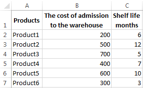
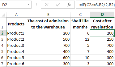
To solve the problem, use the logical IF function. The formula will have a look like this: =IF(C2>=8;B2/2;B2)

Logical expression «C2>=8» is constructed using relational operators «>» and «=». The result of his calculations is a logical value of «TRUE» or «FALSE». In the first case, the function returns the value «B2/2». In the second it’s «B2».

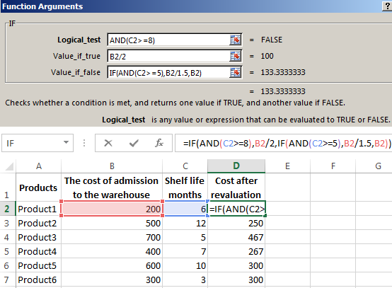
Let’s complicate the task — to employ the logic function И. Now we have such a condition: if the product is stored for more than 8 months, the price is reduced 2 times. If it’s more than 5 months, but less than 8, it’s 1.5 times.

The formula takes the following form:

IF.

The use of logic functions in Excel:

Function Name	Value	Syntax	Note
TRUE	It does not have arguments, it returns the logical value » TRUE «	TRUE	It is rarely used as an independent function
FALSE	It does not have arguments, it returns the logical value » FALSE «	FALSE	——-//——-
AND	If all the given arguments return true result, then the function issues a logical expression » TRUE «. If one of the function outputs the result «false» the whole function gives the result «FALSE»	=AND(boolean1;boolean2;…)	Accepts up to 255 arguments in the form of conditions or links. It is mandatory to first.
OR	It displays the result “TRUE“ if at least one of the arguments is true.	=OR(boolean1;boolean2;…)	——-//——-
NOT	It changes the logic value “TRUE on the contrary — » FALSE «. And vice versa.	#NAME?	Usually it is combined with other operators.
IF	Test the validity of a logical expression and returns the result	=IF (boolean;value_if_TRUE;value_if_FALSE)	« boolean » in the calculations should have results “ TRUE “ or “ FALSE “
IFERROR	If the first argument is true, it returns its argument. Otherwise it’s the value of the second argument.	= IFERROR(value;”error”)	Both arguments are mandatory.

The function IF can be used as arguments to the text values

Objective 2. If the value of the goods in the warehouse after the write-down was less than 300 r. or the product is stored for longer than 10 months, it is written off.

For the solution use logic functions IF and OR:

Condition recorded using a logical OR operation, stands as follows: goods are deducted if the number in cell D2 = 10.

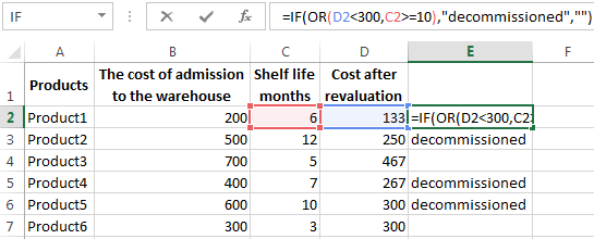
In terms of non-compliance with the conditions, IF function returns to an empty cell.

As arguments, you can use other functions. These are mathematical, for example.

Objective 3. Students before entering the gymnasium pass math, English and Russian. Passing Score is 12. You should get at least 4 points in mathematics for admission. Create report on the receipt.

We set up a table with the source data:

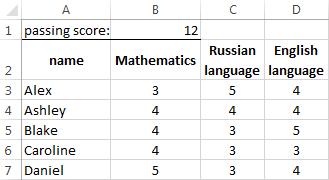
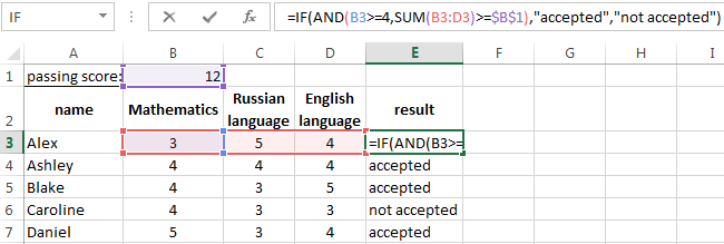
It is necessary to compare the total number of points with a passing grade. And check that math score was not lower than «4». In the «result» column put «accepted» or «not accepted».

There’s such a formula:

Logical operator «AND» causes the function to check the validity of the two conditions. The mathematical function «SUM» is used to calculate the final score.

AND.

The function IF allows us to solve many problems; it is therefore used more often.

The statistical and logical functions in Excel

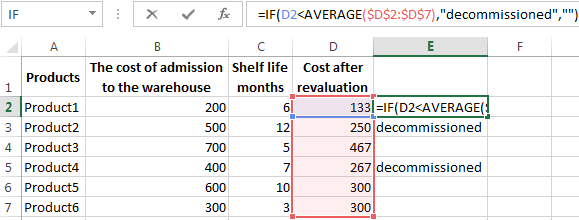
Task 1. Analyze the cost of cash balances after the devaluation. If the price of the product after reassessment is below average values, we should write off the product from the warehouse.

Working with the table in the previous section:

To solve the problem use the formula of such a form:

In logical terms «D2<AVERAGE (D2:D7)» apply statistical function AVERAGE. It returns the average of the range D2: D7.

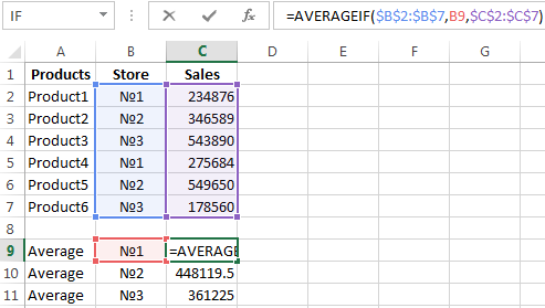
Task 2. Find the average sales in stores.

We set up a table with the source data:

table.

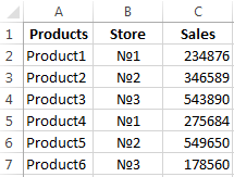
You need to find the arithmetic meaning for the cells, which value corresponds to a predetermined condition. That is to combine logical and statistical solution.

Below a table with a condition there’s the table to display the results.

We solve the problem with a single function:

The first argument $B$2:$B$7 is a range of cells for testing. The second argument B9 is a condition. The third argument the $C$2:$C$7 is an averaging range; the numerical values, which are taken to calculate the arithmetic mean.

AVERAGEIF function compares the value of B9 cells (№1) with values in the range B2: B7. That is the number of stores in the sales table. For matching the data considers the arithmetic mean of using numbers in the range C2: C7.

Task 3. Find the average sales in the store №1 New York and №2 Los Angeles.

Modify the table from the previous example:

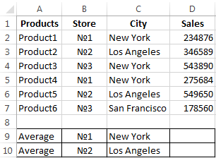
It is necessary to fulfill two conditions — use the function of the form:

Done.

Download examples logical functions

The function AVERAGEIFS allows you to use more than one condition. The first argument $D$2:$D$7 is an averaging ranges (where are the numbers to find the arithmetic mean). The second argument $B$2:$B$7 is a range to test the first condition. The third argument B9 is the first condition. The fourth and fifth arguments are the ranges for checking the second condition respectively.

The function takes into account only the values that meet all these criteria.

Источник

Logical functions in Excel help make comparisons and arrive at a logical conclusion. Here are the logical functions available in Excel and how to use them with examples.

List of Logical Functions

Let’s go over the list of logical functions that are available in excel and learn how we can use them in our day-to-day work.

1. AND function

AND function is one of the logical functions in Excel, which determines whether all criteria in a test are TRUE. it returns TRUE if all of its parameters are TRUE, and FALSE if one or more arguments are FALSE.

Syntax: AND(logical1, [logical2], …), where logical1 is the first condition you want to test is one that can be TRUE or FALSE and logical2… are optional and additional conditions up to a maximum of 255 conditions.

The following example shows the use of AND function:

Select the cell where you want to display the result.
Type =AND(A1>50,B1<50) where cells A1 and B1 contain numeric values.

Press the Enter key to display the result.

2. FALSE function

The FALSE function in Excel returns the logical FALSE value.

Syntax: FALSE(), it has no arguments. Microsoft Excel will read the word FALSE without parentheses as the logical value FALSE if you write it directly onto the worksheet or into a formula.

3. IF function

One of Excel’s most used tools is the IF function, which allows you to create logical comparisons. An IF statement can have two possible outcomes. If the comparison is TRUE, the first result is returned; if the comparison is FALSE, the second result is returned.

Syntax: IF(logical_test,value_if_true,[value_if_false]), where logical_test is the comparison you want to test, value_if_true is the value to be returned if the logical_test is TRUE, and value_if_false is the value to b returned if the logical_test is FALSE. The following example shows the use of the IF function:

Select the cell where you want to display the result.
Type =IF(A1>B1,”A1>B1″,”A1<B1″) where cells A1 and B1 contain numeric values.

Press the Enter key to display the result.

4. IFERROR function

The IFERROR function can be used to catch and manage errors in a formula. If a formula evaluates to an error, IFERROR returns a value you specify; otherwise, it returns the formula’s result.

Syntax: IFERROR(value, value_if_error), where value is the condition to be checked for #N/A, #VALUE!, #REF!, #DIV/0!, #NUM!, #NAME?, or #NULL! error and value_error is the custom message to be returned if the formula evaluates to an error. The following example shows the use of the IFERROR function:

Select the cell where you wan to display the result.
Type =IFERROR(A2/B2,”Error in calculation”) where cells A2 and B2 contain the dividend and divisor respectively.

Press the Enter key to display the result. As, you can see the divisor is zero, so a #DIV/0! should be returned. IFERROR fucntion catches the error and returns the custom message.

5. IFS function

The IFS function determines whether one or more criteria are met and returns the value corresponding to the first TRUE condition. With several criteria, IFS can replace nested IF statements and is considerably easier to read.

Syntax: IFS(logical_test1, value_if_true1, [logical_test2, value_if_true2], [logical_test3, value_if_true3],…), where logical_test1 is the first comparison you want to test, value_if_true 1 is the value to be returned if the logical_test1 is TRUE and the same follows for other conditions. The following example shows the use of IFS function:

Select the cell where you want to display the result.
Type =IFS(A2>89,”A”,A2>79,”B”,A2>69,”C”,A2>59,”D”,A2<=59,”F”) to assign letter grades on the basis of marks obtained.

Press the Enter key to display the result. The value returned is “B” as 85>79 and 85<90.

6. NOT function

The NOT function returns the inverse of its argument’s value. It is frequently used to extend the utility of other functions that perform logical tests.

Syntax: NOT(logical), where logical is a value or expression that may be tested to determine whether it is TRUE or FALSE. The following example shows the use of the NOT function:

Select the cell where you want to display the result.
Type =NOT(TRUE), to reverse TRUE value to FALSE.

Press the Enter key to display the result.

7. OR function

The OR function returns TRUE if any of its parameters are TRUE and FALSE if all of its arguments are FALSE.

Syntax: OR(logical1, [logical2], …), where logical1, logical2, logical3 etc, are conditions to be evaluated for TRUE and FALSE values. The following example shows the use of the OR function:

Select the cell where you want to display the result.
Type =OR(A1<50,B1>50) where cells A1 and B1 contain numeric values.

Press the Enter key to display the result.

8. SWITCH function

The SWITCH function compares one value called the expression to a list of values and returns the first matched value as the result. If no match is found, a default value is returned.

Syntax: SWITCH(expression, value1, result1, [default or value2, result2],…[default or value3, results]), where expression is the value to be compared, value1… are the values to compare an expression to, and result1… are the results to be returned corresponding to the matching value of the expression. The following example shows the use of the SWITCH function:

Select the cell where you want to display the result.
Type =SWITCH(A2,1,”Gold”,2,”Silver”,3,”Bronze”) to decide medals on the basis of rank in cell A2.

Press the Enter key to display the result.

9. TRUE function

The TRUE function in Excel returns the logical TRUE value.

Syntax: TRUE(), it has no arguments. Microsoft Excel will read the word TRUE without parentheses as the logical value TRUE if you write it directly onto the worksheet or into a formula.

10. XOR function

The XOR function returns a TRUE value when the number of true inputs is odd otherwise it returns FALSE. Syntax: XOR(logical1, [logical2],…), where logical1, logical2, logical3 etc, are conditions to be evaluated for TRUE or FALSE values. The following example shows the use of XOR function:

Select the cell where you want to display the result.
Type =XOR(A1>50,B1<50,C1<25) where cells A1, B1 and C1 contain numeric values.

Press the Enter key to display the result. The XOR fucntion returns FALSE value as 2 conditions are TRUE and 2 is an even number.

Conclusion

In this article, we learned about the various logical functions in Excel.

References

AND function (microsoft.com)
FALSE function (microsoft.com)
IF function (microsoft.com)
IFERROR function (microsoft.com)
IFS function (microsoft.com)
NOT function (microsoft.com)
OR function (microsoft.com)
SWITCH function (microsoft.com)
TRUE function (microsoft.com)
XOR function (microsoft.com)

Источник

Содержание

Основные операторы
- Функции ИСТИНА и ЛОЖЬ
- Функции И и ИЛИ
- Функция НЕ
- Функции ЕСЛИ и ЕСЛИОШИБКА
- Функции ЕОШИБКА и ЕПУСТО
Пример применения функций
Вопросы и ответы

Среди множества различных выражений, которые применяются при работе с Microsoft Excel, следует выделить логические функции. Их применяют для указания выполнения различных условий в формулах. При этом, если сами условия могут быть довольно разнообразными, то результат логических функций может принимать всего два значения: условие выполнено (ИСТИНА) и условие не выполнено (ЛОЖЬ). Давайте подробнее разберемся, что представляют собой логические функции в Экселе.

Основные операторы

Существует несколько операторов логических функций. Среди основных следует выделить такие:

ИСТИНА;
ЛОЖЬ;
ЕСЛИ;
ЕСЛИОШИБКА;
ИЛИ;
И;
НЕ;
ЕОШИБКА;
ЕПУСТО.

Существуют и менее распространенные логические функции.

У каждого из вышеуказанных операторов, кроме первых двух, имеются аргументы. Аргументами могут выступать, как конкретные числа или текст, так и ссылки, указывающие адрес ячеек с данными.

Функции ИСТИНА и ЛОЖЬ

Оператор ИСТИНА принимает только определенное заданное значение. У данной функции отсутствуют аргументы, и, как правило, она практически всегда является составной частью более сложных выражений.

Оператор ЛОЖЬ, наоборот, принимает любое значение, которое не является истиной. Точно так же эта функция не имеет аргументов и входит в более сложные выражения.

Функции И и ИЛИ

Функция И является связующим звеном между несколькими условиями. Только при выполнении всех условий, которые связывает данная функция, она возвращает значение ИСТИНА. Если хотя бы один аргумент сообщает значение ЛОЖЬ, то и оператор И в целом возвращает это же значение. Общий вид данной функции: =И(лог_значение1;лог_значение2;…) . Функция может включать в себя от 1 до 255 аргументов.

Функция ИЛИ, наоборот, возвращает значение ИСТИНА даже в том случае, если только один из аргументов отвечает условиям, а все остальные ложные. Её шаблон имеет следующий вид: =И(лог_значение1;лог_значение2;…) . Как и предыдущая функция, оператор ИЛИ может включать в себя от 1 до 255 условий.

Функция НЕ

В отличие от двух предыдущих операторов, функция НЕ имеет всего лишь один аргумент. Она меняет значение выражения с ИСТИНА на ЛОЖЬ в пространстве указанного аргумента. Общий синтаксис формулы выглядит следующим образом: =НЕ(лог_значение) .

Функции ЕСЛИ и ЕСЛИОШИБКА

Для более сложных конструкций используется функция ЕСЛИ. Данный оператор указывает, какое именно значение является ИСТИНА, а какое ЛОЖЬ. Его общий шаблон выглядит следующим образом: =ЕСЛИ(логическое_выражение;значение_если_истина;значение_если-ложь) . Таким образом, если условие соблюдается, то в ячейку, содержащую данную функцию, заполняют заранее указанные данные. Если условие не соблюдается, то ячейка заполняется другими данными, указанными в третьем по счету аргументе функции.

Оператор ЕСЛИОШИБКА, в случае если аргумент является истиной, возвращает в ячейку его собственное значение. Но, если аргумент ошибочный, тогда в ячейку возвращается то значение, которое указывает пользователь. Синтаксис данной функции, содержащей всего два аргумента, выглядит следующем образом: =ЕСЛИОШИБКА(значение;значение_если_ошибка) .

Урок: функция ЕСЛИ в Excel

Функции ЕОШИБКА и ЕПУСТО

Функция ЕОШИБКА проверяет, не содержит ли определенная ячейка или диапазон ячеек ошибочные значения. Под ошибочными значениями понимаются следующие:

#Н/Д;
#ЗНАЧ;
#ЧИСЛО!;
#ДЕЛ/0!;
#ССЫЛКА!;
#ИМЯ?;
#ПУСТО!

В зависимости от того ошибочный аргумент или нет, оператор сообщает значение ИСТИНА или ЛОЖЬ. Синтаксис данной функции следующий: = ЕОШИБКА(значение) . В роли аргумента выступает исключительно ссылка на ячейку или на массив ячеек.

Оператор ЕПУСТО делает проверку ячейки на то, пустая ли она или содержит значения. Если ячейка пустая, функция сообщает значение ИСТИНА, если ячейка содержит данные – ЛОЖЬ. Синтаксис этого оператора имеет такой вид: =ЕПУСТО(значение) . Так же, как и в предыдущем случае, аргументом выступает ссылка на ячейку или массив.

Пример применения функций

Теперь давайте рассмотрим применение некоторых из вышеперечисленных функций на конкретном примере.

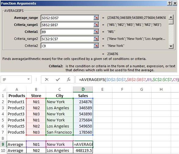
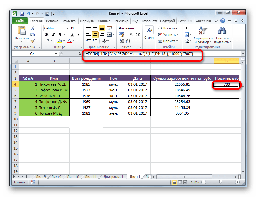
Имеем список работников предприятия с положенными им заработными платами. Но, кроме того, всем работникам положена премия. Обычная премия составляет 700 рублей. Но пенсионерам и женщинам положена повышенная премия в размере 1000 рублей. Исключение составляют работники, по различным причинам проработавшие в данном месяце менее 18 дней. Им в любом случае положена только обычная премия в размере 700 рублей.

Попробуем составить формулу. Итак, у нас существует два условия, при исполнении которых положена премия в 1000 рублей – это достижение пенсионного возраста или принадлежность работника к женскому полу. При этом, к пенсионерам отнесем всех тех, кто родился ранее 1957 года. В нашем случае для первой строчки таблицы формула примет такой вид: =ЕСЛИ(ИЛИ(C4<1957;D4="жен.");"1000";"700") . Но, не забываем, что обязательным условием получения повышенной премии является отработка 18 дней и более. Чтобы внедрить данное условие в нашу формулу, применим функцию НЕ: =ЕСЛИ(ИЛИ(C4<1957;D4="жен.")*(НЕ(E4<18));"1000";"700") .

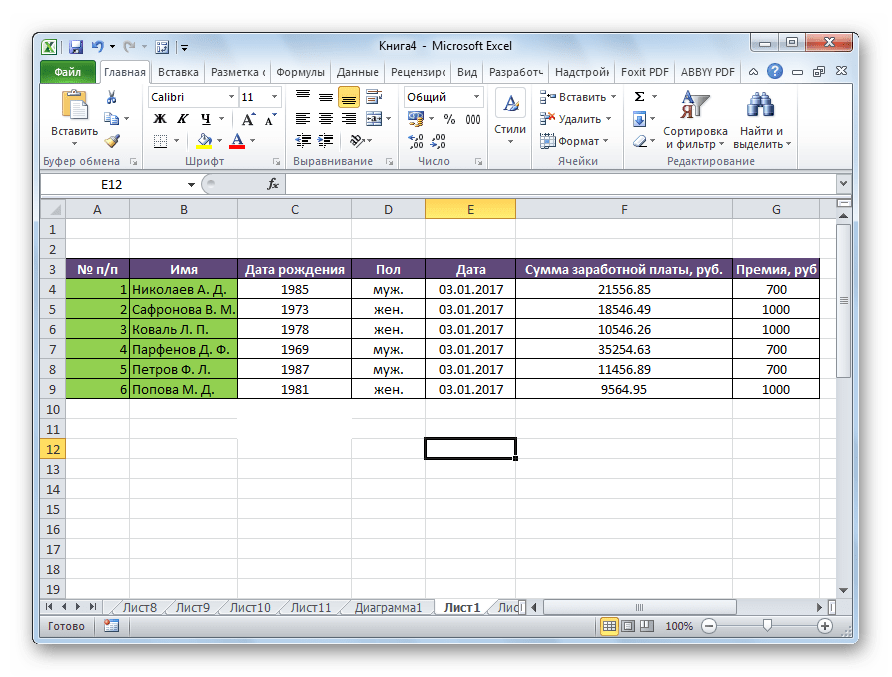
Для того, чтобы скопировать данную функцию в ячейки столбца таблицы, где указана величина премии, становимся курсором в нижний правый угол ячейки, в которой уже имеется формула. Появляется маркер заполнения. Просто перетягиваем его вниз до конца таблицы.

Таким образом, мы получили таблицу с информацией о величине премии для каждого работника предприятия в отдельности.

Урок: полезные функции Excel

Как видим, логические функции являются очень удобным инструментом для проведения расчетов в программе Microsoft Excel. Используя сложные функции, можно задавать несколько условий одновременно и получать выводимый результат в зависимости от того, выполнены эти условия или нет. Применение подобных формул способно автоматизировать целый ряд действий, что способствует экономии времени пользователя.

Источник

What is IF Function in Excel?

Table of contents

Syntax of the IF Excel Function

How to Use IF Function in Excel?

Example #1

Example #2

Example #3

Example #4

Example #5

Guidelines for the Multiple IF Statements

Frequently Asked Question

IF Excel Function Video

Recommended Articles

Logical functions in Excel and examples of solving the problems

The use of logic functions in Excel:

The function IF can be used as arguments to the text values

The statistical and logical functions in Excel

List of Logical Functions

1. AND function

2. FALSE function

3. IF function

4. IFERROR function

5. IFS function

6. NOT function

7. OR function

8. SWITCH function

9. TRUE function

10. XOR function

Conclusion

References

Основные операторы

Функции ИСТИНА и ЛОЖЬ

Функции И и ИЛИ

Функция НЕ

Функции ЕСЛИ и ЕСЛИОШИБКА

Функции ЕОШИБКА и ЕПУСТО

Пример применения функций