
В этом уроке мы познакомимся с самым объемным и часто посещаемым разделом Microsoft Excel – Библиотекой функций. Мы рассмотрим структуру библиотеки, из каких категорий и команд она состоит. К каждой категории приведено небольшое описание, которое даст Вам общее представление о предназначении функций, входящих в библиотеку. В конце урока мы на примере разберем, как вставить функцию из библиотеки.
В Microsoft Excel имеются сотни самых различных функций, которые делятся по категориям. Все эти функции составляют общую библиотеку. Вам нет необходимости досконально изучать каждую функцию, но познакомиться с несколькими основными из каждой категории будет весьма полезно.
Содержание
- Как получить доступ к библиотеке
- Вставить функцию
- Автосумма
- Последние
- Финансовые
- Логические
- Текстовые
- Дата и время
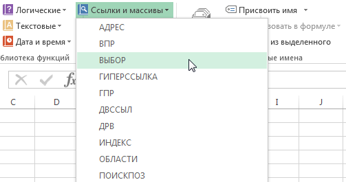
- Ссылки и массивы
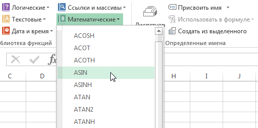
- Математические
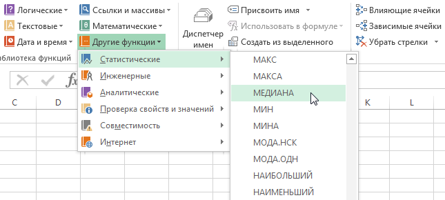
- Другие функции
- Как вставить функцию из библиотеки
Как получить доступ к библиотеке
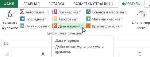
Чтобы получить доступ к библиотеке функций Excel, выберите вкладку Формулы. Все возможные категории и команды вы можете увидеть в группе Библиотека функций.
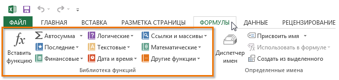
Разберем, какую задачу выполняет каждая из команд группы:
Вставить функцию
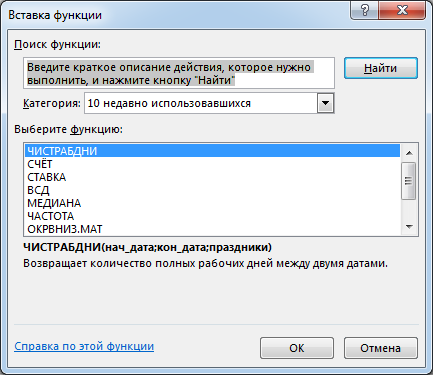
Если у Вас возникли проблемы с поиском необходимой функции в Excel, команда Вставить функцию позволяет найти ее при помощи ключевых слов.
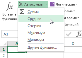
Автосумма
Команда Автосумма позволяет автоматически вычислять результаты для наиболее распространенных функций Excel, таких как СУММ, СРЗНАЧ, СЧЕТ, МАКС и МИН.
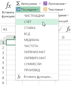
Последние
Команда Последние дает доступ к функциям Excel, с которыми Вы работали недавно.
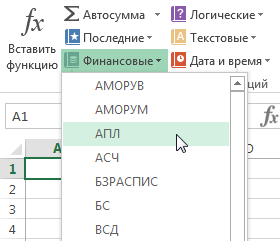
Финансовые
Категория Финансовые содержит функции для финансовых расчетов, например, сумма периодического платежа ПЛТ или процентная ставка по кредиту СТАВКА.
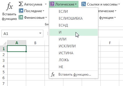
Логические
Функции из категории Логические используются для проверки аргументов на соответствие определенному значению или условию. Например, если сумма заказа меньше $50, то добавляется цена доставки $4.99, а если больше, то стоимость доставки не взимается. В данном примере целесообразно использовать функцию ЕСЛИ.
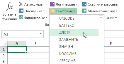
Текстовые
В категории Текстовые содержатся функции, которые работают с текстом в качестве значений аргументов. С помощью них можно решать такие задачи, как преобразование текста в нижний регистр (СТРОЧН) или замена части текста на другое значение (ЗАМЕНИТЬ).
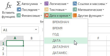
Дата и время
Категория Дата и время содержит функции для работы с датами и временем в формулах. Например, функция СЕГОДНЯ возвращает текущую дату, а функция ТДАТА дополнительно к дате еще и время.
Ссылки и массивы
В категории Ссылки и массивы содержатся функции, которые предназначены для просмотра и поиска информации. Например, Вы можете добавить гиперссылку (ГИПЕРССЫЛКА) в ячейку или вернуть значение, которое расположено на пересечении заданных строки и столбца (ИНДЕКС).
Математические
Категория Математические включает в себя функции для обработки числовых аргументов, выполняющие различные математические и тригонометрические вычисления. Например, вы можете округлить значение (ОКРУГЛ), найти значение Пи (ПИ), произведение (ПРОИЗВЕД), промежуточные итоги (ПРОМЕЖУТОЧНЫЕ.ИТОГИ) и многое другое.
Другие функции
Раздел Другие функции содержит дополнительные категории библиотеки функций, такие как Статистические, Инженерные, Аналитические, Проверка свойств и значений, а также функции, оставленные для поддержки совместимости с предыдущими версиями Excel.
Как вставить функцию из библиотеки
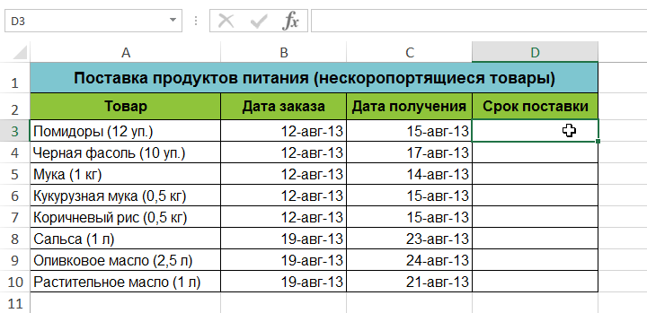
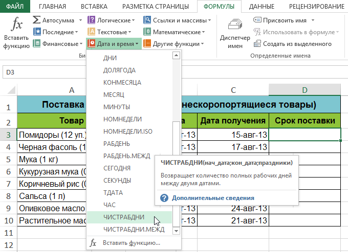
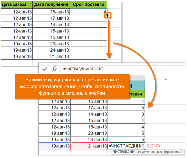
В следующем примере Вы увидите, как вставить функцию из библиотеки Excel, позволяющую вычислить количество рабочих дней, в течение которых должна быть произведена доставка товара. В нашем случае мы будем использовать данные в столбцах B и C для расчета времени доставки.
- Выделите ячейку, которая будет содержать формулу. В нашем примере это ячейка D3.

- Выберите вкладку Формулы на Ленте, чтобы открыть Библиотеку функций.
- В группе команд Библиотека функций, выберите нужную категорию. В нашем случае мы выберем Дата и время.
- Выберите нужную функцию из выпадающего меню. Мы выберем функцию ЧИСТРАБДНИ, чтобы вычислить количество рабочих дней между датами заказа и получения товара.
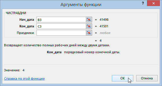
- Появится диалоговое окно Аргументы функции. Здесь вы можете ввести или выбрать ячейки, которые будут составлять аргументы. Мы введем B3 в поле Нач_дата и С3 в поле Кон_дата.
- Если аргументы введены правильно, нажмите ОК.
- Функция будет вычислена, и Вы увидите результат. Результат показывает, что доставка заказа заняла 4 рабочих дня.
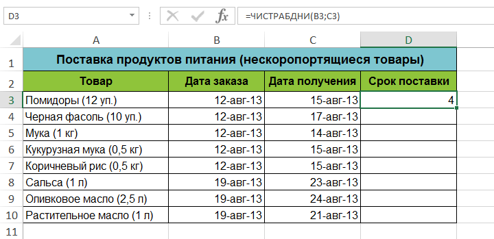
Так же, как и формулы, функции в Excel могут быть скопированы в смежные ячейки. Наведите курсор на ячейку, которая содержит функцию. Затем нажмите левую кнопку мыши и, не отпуская ее, перетащите маркер автозаполнения по ячейкам, которые необходимо заполнить. Функция будет скопирована, а значения вычислены в зависимости от строк или столбцов.
Оцените качество статьи. Нам важно ваше мнение:
Нет, RefEditControl работает нормально.
Missing выходит (на ноутбуке) на Microsoft Visual Studo for Application 2.0 Project Package 9.0 Type Library.
Вернее, это у меня стоит на компе и всё работает, Missing появляется на ноутбуке.
Интересно, что происходит при сбросе флажка? Библиотека отключается? Т.е. она не нужна? Откуда же она появилась на компе — стоит по умолчанию.
Для проверки сбросил флаг на компе — работает по прежнему.
Немного прояснилось — эту библиотеку воткнул Excel, но она здесь не нужна.
Но почему же она Missing на ноутбуке, если там стоит тот же самый Office?
Единственно, устанавливался по разному. На компе я устанавливал «тихой установкой», а на компе «явной».
Ну и Windows разные — на компе Десятка, на ноутбуке Семёрка
Добавлено через 13 минут
Hugo121, Вы совершенно правы.
Но с другой стороны — откуда я мог знать, какие там библиотеки лишние, какие нет?
Я же просто пишу код и больше ничего.
По той ссылке, что я привёл, есть маленькая процедура, которая снимает флаги с библиотек, которые Missing.
Думаю, не будет преступлением, если я её здесь приведу:
| Visual Basic | ||
|
Далее приведён следующий текст:
Но для работы этого макроса необходимо:
проставить доверие к проекту VBA:
Excel 2010 — Файл-Параметры-Центр управления безопасностью-Параметры макросов-поставить галочку «Доверять доступ к объектной модели проектов VBA»
Excel 2007 — Кнопка Офис-Параметры Excel-Центр управления безопасностью-Параметры макросов-поставить галочку «Доверять доступ к объектной модели проектов VBA»
Excel 2003- Сервис — Параметры-вкладка Безопасность-Параметры макросов-Доверять доступ к Visual Basic Project
проект VBA не должен быть защищен.
Так же Can’t find project or library возникает если у Вас просто не подключена какая-либо библиотека, которая используется в коде. Тогда не будет MISSING. Надо просто определить, в какую библиотеку входит константа, объект или свойство, которое выделяет редактор при выдаче ошибки, и подключить эту библиотеку.
Только в MS Office 2013 стоит не «Параметры макросов — Доверять доступ к объектной модели проектов VBA», а «Параметры центра по управлению безопасностью — Предоставлять доступ к объектной модели проектов VBA»
So I’m having to run someone else’s excel app on my PC, and I’m getting «Can’t find Project or Library» on standard functions such as date, format, hex, mid, etc.
Some research indicates that if I prefix these functions with «VBA.» as in «VBA.Date» then it’ll work fine.
Webpages suggest it has to do with my project references on my system, whereas they must be ok on the developer’s system. I’m going to be dealing with this for some time from others, and will be distributing these applications to many others, so I need to understand what’s wrong with my excel setup that I need to fix, or what needs to be changed in the xls file so that it’ll run on a variety of systems. I’d like to avoid making everyone use «VBA.» as an explicit reference, but if there’s no ideal solution I suppose that’s what we’ll have to do.
- How do I make «VBA.» implicit in my project properties/references/etc?
-Adam
![]()
Vincent
4173 silver badges11 bronze badges
asked Feb 3, 2009 at 14:05
![]()
Adam DavisAdam Davis
91.4k59 gold badges262 silver badges330 bronze badges
5
I have seen errors on standard functions if there was a reference to a totally different library missing.
In the VBA editor launch the Compile command from the menu and then check the References dialog to see if there is anything missing and if so try to add these libraries.
In general it seems to be good practice to compile the complete VBA code and then saving the document before distribution.
answered Feb 3, 2009 at 14:24
![]()
Dirk VollmarDirk Vollmar
171k53 gold badges256 silver badges313 bronze badges
5
I had the same problem. This worked for me:
- In VB go to Tools » References
- Uncheck the library «Crystal Analysis Common Controls 1.0». Or any library.
- Just leave these 5 references:
- Visual Basic For Applications (This is the library that defines the VBA language.)
- Microsoft Excel Object Library (This defines all of the elements of Excel.)
- OLE Automation (This specifies the types for linking and embedding documents and for automation of other applications and the «plumbing» of the COM system that Excel uses to communicate with the outside world.)
- Microsoft Office (This defines things that are common to all Office programs such as Command Bars and Command Bar controls.)
- Microsoft Forms 2.0 This is required if you are using a User Form. This library defines things like the user form and the controls that you can place on a form.
- Then Save.
![]()
JimmyPena
8,6986 gold badges43 silver badges64 bronze badges
answered Jul 8, 2011 at 14:18
![]()
3
I have experienced this exact problem and found, on the users machine, one of the libraries I depended on was marked as «MISSING» in the references dialog. In that case it was some office font library that was available in my version of Office 2007, but not on the client desktop.
The error you get is a complete red herring (as pointed out by divo).
Fortunately I wasn’t using anything from the library, so I was able to remove it from the XLA references entirely. I guess, an extension of divo’ suggested best practice would be for testing to check the XLA on all the target Office versions (not a bad idea in any case).
answered Mar 4, 2009 at 22:44
![]()
RedBlueThingRedBlueThing
41.7k17 gold badges98 silver badges122 bronze badges
In my case, it was that the function was AMBIGUOUS as it was defined in the VBA library (present in my references), and also in the Microsoft Office Object Library (also present). I removed the Microsoft Office Object Library, and voila! No need to use the VBA. prefix.
answered Jul 11, 2009 at 14:14
blue_wardrobeblue_wardrobe
In my case, I could not even open «References» in the Visual Basic window. I even tried reinstalling Office 365 and that didn’t work. Finally, I tried disabling macros in the «Trust Center» settings. When I restarted Excel, I got the warning message that macros were disabled, and when I clicked on «enable» I no longer got the error message.
Later I re-enabled all macros in the «Trust Center» settings, and the error message didn’t show up!
Hey, if nothing else works for you, try the above; it worked for me! 
Update:
The issue returned, and this is how I «fixed» it the second time:
I opened my workbook in Excel online (Office 365, in the browser, which doesn’t support macros anyway), saved it with a new file name (still using .xlsm file extension), and reopened in the desktop software. It worked.
answered Feb 5, 2020 at 1:09
![]()
Sean McCarthySean McCarthy
4,6308 gold badges38 silver badges55 bronze badges
2
Even when all references are fine the prefix problem causes compile errors.
What about creating a find and replace sub for all ‘built-in VBA functions’ in all modules,
like this:
replace text in code module
e.g. «= Date» will be replaced with «= VBA.Date».
e.g. » Date(» will be replaced with » VBA.Date(» .
(excluding «dim t As Date» or «mydate»)
All vba functions for find and replace are written here :
vba functions list
answered Dec 4, 2020 at 22:30
![]()
Noam BrandNoam Brand
3152 silver badges13 bronze badges
For those of you who haven’t found any of the other answers work for you.
Try this:
Close out of the file, email it to yourself or if you’re at work, paste it from the network drive to your desktop, anything to get it to open in «protected mode».
Now open the file
DON’T CLICK ANY ENABLE EDITING OR THE YELLOW RIBBON
Go to the VBA Editor
Go to Debug — — Compile VBA Project, if «Compile VBA Project» is greyed out, then you may need to click the yellow ribbon one time to enable the content, but DO NOT enable macros.
After you click Compile, save, close out of the file. Reopen it, enable everything and it should be OK. This has worked for me 100% of the time.
answered Nov 3, 2021 at 19:27
![]()
In my case I was checking work done on my office computer (with Visio installed) at home (no Visio). Even though VBA appeared to be getting hung up on simple default functions, the problem was that I had references to the Visio libraries still active.
answered Feb 5, 2018 at 10:47
![]()
SmrtGruntSmrtGrunt
84913 silver badges24 bronze badges
I found references to an AVAYA/CMS programme file? Totally random, this was in MS Access, nothing to do with AVAYA. I do have AVAYA on my PC, and others don’t, so this explains why it worked on my machine and not others — but not how Access got linked to AVAYA. Anyway — I just unchecked the reference and that seems to have fixed the problem
answered Oct 9, 2019 at 8:10
![]()
I’ve had this error on and off for around two years in a several XLSM files (which is most annoying as when it occurs there is nothing wrong with the file! — I suspect orphaned Excel processes are part of the problem)
The most efficient solution I had found has been to use Python with oletools
https://github.com/decalage2/oletools/wiki/Install and extract the VBA code all the modules and save in a text file.
Then I simply rename the file to zip file (backup just in case!), open up this zip file and delete the xl/vbaProject.bin file. Rename back to XLSX and should be good to go.
Copy in the saved VBA code (which will need cleaning of line breaks, comments and other stuff. Will also need to add in missing libraries.
This has saved me when other methods haven’t.
YMMV.
answered Sep 21, 2020 at 7:50
![]()
Содержание
- Фильтры и сортировка в Microsoft Excel
- Функционал фильтрации и сортировки в Microsoft Excel
- Сортировка данных в Microsoft Excel
- Фильтрация данных в Microsoft Excel
- Sort data in a range or table
- Sort text
Фильтры и сортировка в Microsoft Excel
MS Excel – это мощнейший табличный редактор, и у него огромнейший арсенал возможностей по работе с данными. В числе этих возможностей – сортировка и фильтрация. Эти возможности вам пригодятся в работе с разными таблицами, которые содержат большие объёмы данных. Они помогут вам проанализировать значимые данные, отследить тенденции роста и спада их значений, вывести на печать только выборочные позиции таблиц. Давайте рассмотрим, как работают фильтры и сортировка в Microsoft Excel.
Функционал фильтрации и сортировки в Microsoft Excel
У Microsoft Excel несколько реализаций функционала фильтрации и сортировки. Если вы создадите форматированную таблицу, т.е. сделаете обычную таблицу с данными, потом выделите её и форматируете как таблицу,
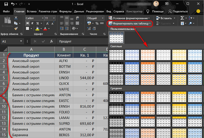
по умолчанию она у вас создастся с интегрированными функциями фильтрации и сортировки. Столбцы с названиями уже будут содержать кнопки выпадающих списков функций фильтрации и сортировки.
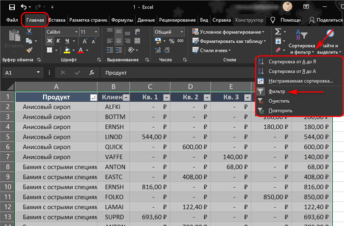
Это не всегда удобно т.к. часто нужно компактное размещение таблицы на листе для вывода на печать. И если вы не будете пользоваться фильтрацией, чтобы эти кнопки не занимали место в названиях таблицы и не отвлекали внимание, их можно убрать. Делаем клик на любой ячейке таблицы, идём в меню «Данные», жмём «Фильтр». И всё – кнопки фильтрации и сортировки убраны из таблицы. Этой же кнопкой «Фильтр» мы можем при необходимости вернуть интеграцию фильтрации и сортировки в таблицу. Либо же можно реализовать её для простой неформатированной таблицы. Если вам необходимо только сортировать данные таблицы, можно сделать это с помощью кнопок для сортировки в меню MS Excel «Данные».
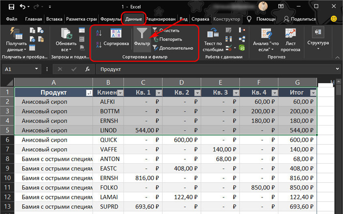
Или в главном меню, всё это один и тот же функционал. Здесь также есть кнопка «Фильтр» для включения/отключения интеграции фильтрации и сортировки в таблицу.
Также функционал фильтрации и сортировки будет доступным в контекстном меню на ячейках таблицы.
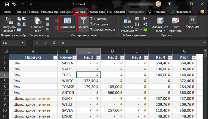
Сортировка данных в Microsoft Excel
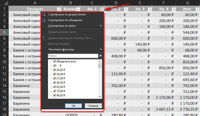
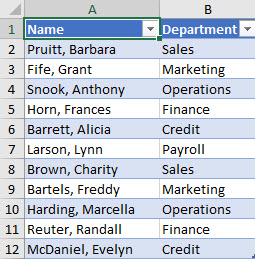
Данные таблицы можно сортировать по возрастанию или убыванию значений ячеек: текстовые — по алфавиту, числовые – по последовательности из чисел, временные – по временной последовательности. Нажимаем на любую из ячеек столбца с данными, по критерию которых мы хотим с вами выстроить таблицу. И жмём в главном меню или меню «Данные» Microsoft Excel кнопку сортировки данных – по возрастанию или убыванию. Если это столбец, например, с ценами, вся таблица выстроится в последовательности увеличения или уменьшения цен в указанном столбце. Если это столбец, скажем, с названиями товаров, таблица выстроится по алфавиту названий товаров в обычном или обратном порядке.
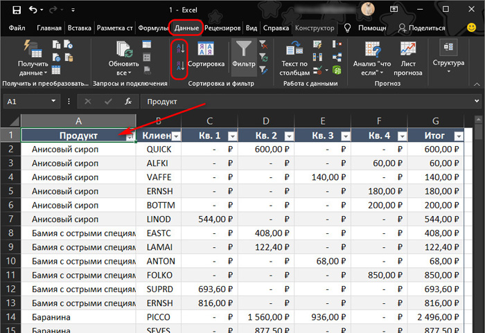
Бóльшие возможности может предложить функция настраиваемой сортировки. Нажмём на данную кнопку.
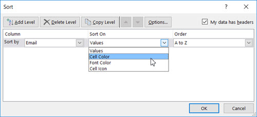
И здесь мы в качестве критериев для сортировки можем выбрать :
- «Столбец» — тип данных таблицы, т.е. столбцы с названиями данных нашей таблицы ;
- «Сортировка» – значения ячеек, выделения цветным маркером или шрифтом, условное форматирование ;
- «Порядок сортировки» – убывание или возрастание.
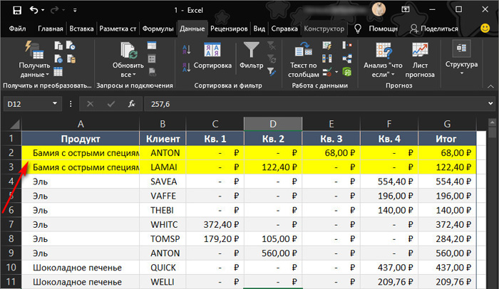
Например, у нас в таблице есть особые позиции товара, которые надо постоянно мониторить, мы их отметили жёлтым маркером. Чтобы отсортировать таблицу по строкам с жёлтым маркером, оставляем первый критерий для сортировки по умолчанию, в нашем случае это столбец наименования товара. Второй критерий сортировки выставим цвет ячейки. Для третьего критерия порядка сортировки указываем жёлтый цвет ячеек. И также указываем, что маркированные данные должны быть сверху списка. Жмём «Ок».
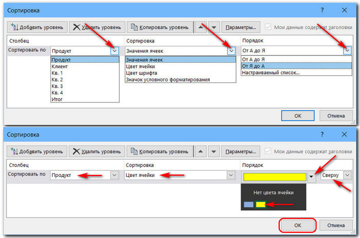
И вот: отмеченные маркером позиции таблицы находятся в самом верху.
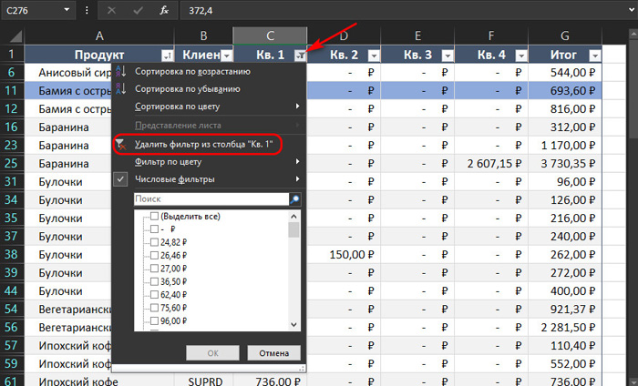
Фильтрация данных в Microsoft Excel
Для фильтрации данных, как упоминалось, нужны интегрированные в таблицу функции фильтрации и сортировки. Если в вашей таблице их нет, повторимся, в главном меню или меню «Данные» Microsoft Excel нужно нажимать на кнопку «Фильтр». Если у вас таблица с большим объёмом данных, с помощью фильтра в таблице Excel можете убрать какие-то строки и оставить лишь нужные. И таким образом сделать информацию более удобной для анализа или печати.
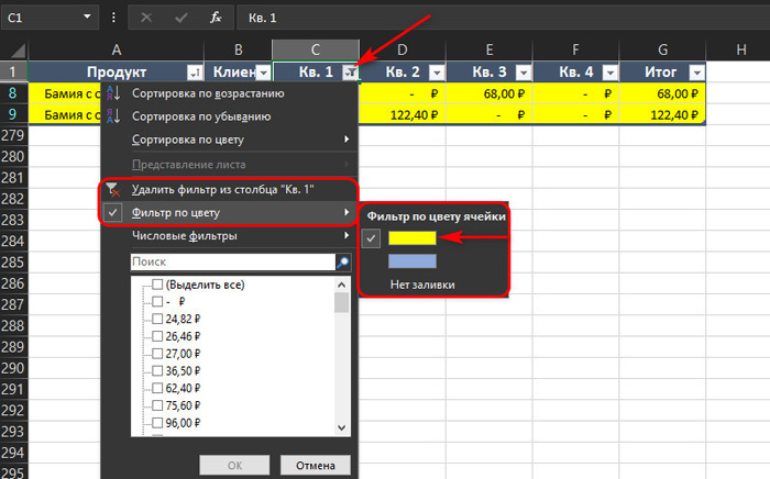
Работает фильтр очень просто: в выпадающем списке столбца с данными, где мы хотим убрать отдельные из них, нажимаем на выпадающий список и работаем с фильтром. Например, вот тот же случай, когда у нас есть отмеченные маркером особо важные позиции таблицы. И чтобы отобразить у нас в таблице только их, в выпадающем списке столбца жмём «Фильтр по цвету». Укажем цвет маркера, в нашем случае жёлтый. И в таблице отобразятся только маркированные данные. Чтобы убрать фильтр, в выпадающем списке этого же столбца нажмём «Удалить фильтр из столбца…».
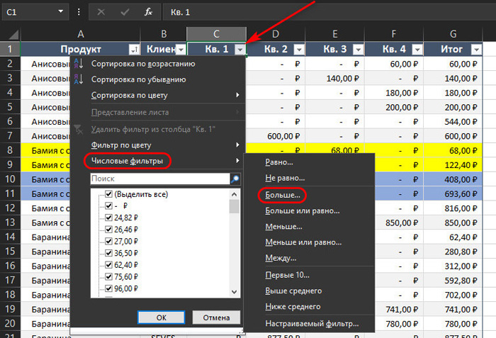
В столбцах с числовыми данными нам будут доступны числовые фильтры. С их помощью можем убрать из таблицы, например, данные с маленькими суммами. Нажмём на выпадающий список столбца с интересующими нас цифрами, жмём «Числовые фильтры», выбираем «Больше».
И укажем цифру, скажем, 100. Т.е. мы хотим скрыть товарные позиции с сумами меньше 100 руб. Вписываем данную цифру или можем выбрать варианты сумм из выпадающего списка фильтра. Жмём «Ок».
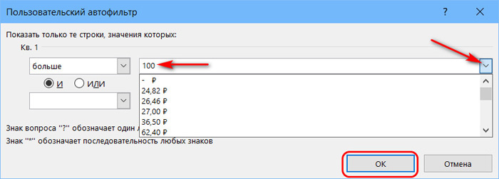
И всё: позиции таблицы с сумами менее 100 руб. теперь скрыты. Чтобы вернуть их назад, удаляем фильтр в этом же столбце.
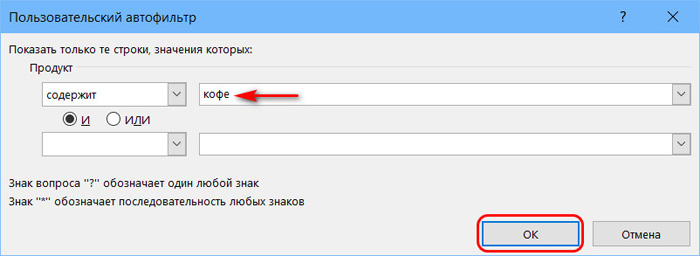
Работа с фильтром текстовых данных аналогична. В столбце с наименованиями позиций товара нажмём выпадающий список, выберем «Текстовые фильтры», жмём «Содержит».
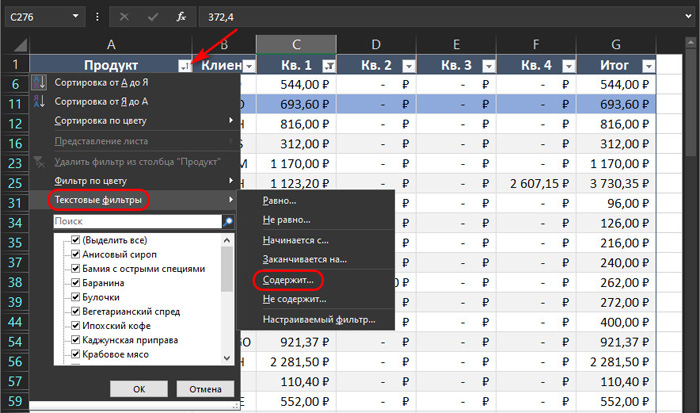
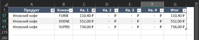
И укажем слово-фильтр. Например, мы хотим видеть в таблице только позиции по кофе. Вписываем слово «кофе», жмём «Ок».
И таблица отфильтрована по этому слову в названиях товаров.
По такому же принципу, мы можем отфильтровать позиции товара, которые не содержат каких-то слов или букв в названиях, начинаются или заканчиваются с каких-то букв. Убирается текстовый фильтр так же, как и цветной и числовой.
Источник
Sort data in a range or table

Sorting data is an integral part of data analysis. You might want to arrange a list of names in alphabetical order, compile a list of product inventory levels from highest to lowest, or order rows by colors or icons. Sorting data helps you quickly visualize and understand your data better, organize and find the data that you want, and ultimately make more effective decisions.
You can sort data by text (A to Z or Z to A), numbers (smallest to largest or largest to smallest), and dates and times (oldest to newest and newest to oldest) in one or more columns. You can also sort by a custom list you create (such as Large, Medium, and Small) or by format, including cell color, font color, or icon set.
To find the top or bottom values in a range of cells or table, such as the top 10 grades or the bottom 5 sales amounts, use AutoFilter or conditional formatting.

Sort text
Select a cell in the column you want to sort.
On the Data tab, in the Sort & Filter group, do one of the following:
To quick sort in ascending order, click  ( Sort A to Z).
To quick sort in descending order, click  ( Sort Z to A).
Notes: Potential Issues
Check that all data is stored as text If the column that you want to sort contains numbers stored as numbers and numbers stored as text, you need to format them all as either numbers or text. If you do not apply this format, the numbers stored as numbers are sorted before the numbers stored as text. To format all the selected data as text, Press Ctrl+1 to launch the Format Cells dialog, click the Number tab and then, under Category, click General, Number, or Text.
Remove any leading spaces In some cases, data imported from another application might have leading spaces inserted before data. Remove the leading spaces before you sort the data. You can do this manually, or you can use the TRIM function.
Select a cell in the column you want to sort.
On the Data tab, in the Sort & Filter group, do one of the following:
To sort from low to high, click ( Sort Smallest to Largest).
To sort from high to low, click ( Sort Largest to Smallest).
Check that all numbers are stored as numbers If the results are not what you expected, the column might contain numbers stored as text instead of as numbers. For example, negative numbers imported from some accounting systems, or a number entered with a leading apostrophe ( ‘) are stored as text. For more information, see Fix text-formatted numbers by applying a number format.
Select a cell in the column you want to sort.
On the Data tab, in the Sort & Filter group, do one of the following:
To sort from an earlier to a later date or time, click ( Sort Oldest to Newest).
To sort from a later to an earlier date or time, click ( Sort Newest to Oldest).
Notes: Potential Issue
Check that dates and times are stored as dates or times If the results are not what you expected, the column might contain dates or times stored as text instead of as dates or times. For Excel to sort dates and times correctly, all dates and times in a column must be stored as a date or time serial number. If Excel cannot recognize a value as a date or time, the date or time is stored as text. For more information, see Convert dates stored as text to dates.
If you want to sort by days of the week, format the cells to show the day of the week. If you want to sort by the day of the week regardless of the date, convert them to text by using the TEXT function. However, the TEXT function returns a text value, so the sort operation would be based on alphanumeric data. For more information, see Show dates as days of the week.
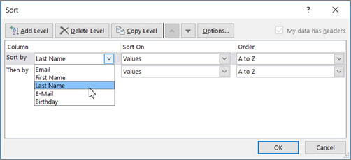
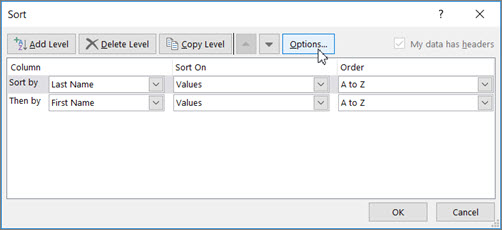
You may want to sort by more than one column or row when you have data that you want to group by the same value in one column or row, and then sort another column or row within that group of equal values. For example, if you have a Department column and an Employee column, you can first sort by Department (to group all the employees in the same department together), and then sort by name (to put the names in alphabetical order within each department). You can sort by up to 64 columns.
Note: For best results, the range of cells that you sort should have column headings.
Select any cell in the data range.
On the Data tab, in the Sort & Filter group, click Sort.

In the Sort dialog box, under Column, in the Sort by box, select the first column that you want to sort.
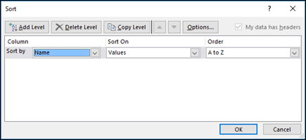
Under Sort On, select the type of sort. Do one of the following:
To sort by text, number, or date and time, select Values.
To sort by format, select Cell Color, Font Color, or Cell Icon.
Under Order, select how you want to sort. Do one of the following:
For text values, select A to Z or Z to A.
For number values, select Smallest to Largest or Largest to Smallest.
For date or time values, select Oldest to Newest or Newest to Oldest.
To sort based on a custom list, select Custom List.
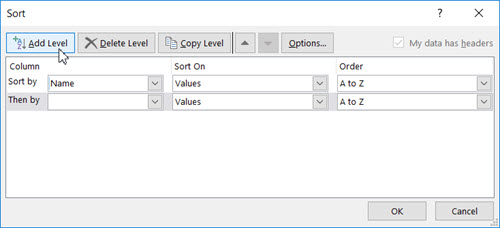
To add another column to sort by, click Add Level, and then repeat steps three through five.
To copy a column to sort by, select the entry and then click Copy Level.
To delete a column to sort by, select the entry and then click Delete Level.
Note: You must keep at least one entry in the list.
To change the order in which the columns are sorted, select an entry and then click the Up or Down arrow next to the Options button to change the order.
Entries higher in the list are sorted before entries lower in the list.
If you have manually or conditionally formatted a range of cells or a table column by cell color or font color, you can also sort by these colors. You can also sort by an icon set that you created with conditional formatting.
Select a cell in the column you want to sort.
On the Data tab, in the Sort & Filter group, click Sort.
In the Sort dialog box, under Column, in the Sort by box, select the column that you want to sort.
Under Sort On, select Cell Color, Font Color, or Cell Icon.
Under Order, click the arrow next to the button and then, depending on the type of format, select a cell color, font color, or cell icon.
Next, select how you want to sort. Do one of the following:
To move the cell color, font color, or icon to the top or to the left, select On Top for a column sort, and On Left for a row sort.
To move the cell color, font color, or icon to the bottom or to the right, select On Bottom for a column sort, and On Right for a row sort.
Note: There is no default cell color, font color, or icon sort order. You must define the order that you want for each sort operation.
To specify the next cell color, font color, or icon to sort by, click Add Level, and then repeat steps three through five.
Make sure that you select the same column in the Then by box and that you make the same selection under Order.
Keep repeating for each additional cell color, font color, or icon that you want included in the sort.
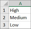
You can use a custom list to sort in a user-defined order. For example, a column might contain values that you want to sort by, such as High, Medium, and Low. How can you sort so that rows containing High appear first, followed by Medium, and then Low? If you were to sort alphabetically, an “A to Z” sort would put High at the top, but Low would come before Medium. And if you sorted “Z to A,” Medium would appear first, with Low in the middle. Regardless of the order, you always want “Medium” in the middle. By creating your own custom list, you can get around this problem.
Optionally, create a custom list:
In a range of cells, enter the values that you want to sort by, in the order that you want them, from top to bottom as in this example.
Select the range that you just entered. Using the preceding example, select cells A1:A3.
Go to File > Options > Advanced > General > Edit Custom Lists, then in the Custom Lists dialog box, click Import, and then click OK twice.
You can create a custom list based only on a value (text, number, and date or time). You cannot create a custom list based on a format (cell color, font color, or icon).
The maximum length for a custom list is 255 characters, and the first character must not begin with a number.
Select a cell in the column you want to sort.
On the Data tab, in the Sort & Filter group, click Sort.
In the Sort dialog box, under Column, in the Sort by or Then by box, select the column that you want to sort by a custom list.
Under Order, select Custom List.
In the Custom Lists dialog box, select the list that you want. Using the custom list that you created in the preceding example, click High, Medium, Low.
On the Data tab, in the Sort & Filter group, click Sort.
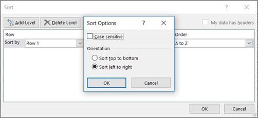
In the Sort dialog box, click Options.
In the Sort Options dialog box, select Case sensitive.
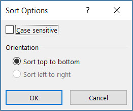
It’s most common to sort from top to bottom, but you can also sort from left to right.
Note: Tables don’t support left to right sorting. To do so, first convert the table to a range by selecting any cell in the table, and then clicking Table Tools > Convert to range.
Select any cell within the range you want to sort.
On the Data tab, in the Sort & Filter group, click Sort.
In the Sort dialog box, click Options.
In the Sort Options dialog box, under Orientation, click Sort left to right, and then click OK.
Under Row, in the Sort by box, select the row that you want to sort. This will generally be row 1 if you want to sort by your header row.
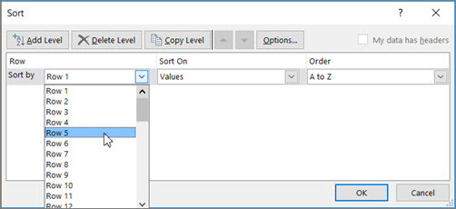
Tip: If your header row is text, but you want to order columns by numbers, you can add a new row above your data range and add numbers according to the order you want them.
To sort by value, select one of the options from the Order drop-down:
For text values, select A to Z or Z to A.
For number values, select Smallest to Largest or Largest to Smallest.
For date or time values, select Oldest to Newest or Newest to Oldest.
To sort by cell color, font color, or cell icon, do this:
Under Sort On, select Cell Color, Font Color, or Cell Icon.
Under Order select a cell color, font color, or cell icon, then select On Left or On Right.
Note: When you sort rows that are part of a worksheet outline, Excel sorts the highest-level groups (level 1) so that the detail rows or columns stay together, even if the detail rows or columns are hidden.
To sort by a part of a value in a column, such as a part number code (789- WDG-34), last name (Carol Philips), or first name (Philips, Carol), you first need to split the column into two or more columns so that the value you want to sort by is in its own column. To do this, you can use text functions to separate the parts of the cells or you can use the Convert Text to Columns Wizard. For examples and more information, see Split text into different cells and Split text among columns by using functions.
Warning: It is possible to sort a range within a range, but it is not recommended, because the result disassociates the sorted range from its original data. If you were to sort the following data as shown, the selected employees would be associated with different departments than they were before.
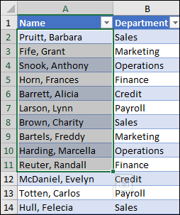
Fortunately, Excel will warn you if it senses you are about to attempt this:

If you did not intend to sort like this, then press the Expand the selection option, otherwise select Continue with the current selection.
If the results are not what you want, click Undo  .
.
Note: You cannot sort this way in a table.
If you get unexpected results when sorting your data, do the following:
Check to see if the values returned by a formula have changed If the data that you have sorted contains one or more formulas, the return values of those formulas might change when the worksheet is recalculated. In this case, make sure that you reapply the sort to get up-to-date results.
Unhide rows and columns before you sort Hidden columns are not moved when you sort columns, and hidden rows are not moved when you sort rows. Before you sort data, it’s a good idea to unhide the hidden columns and rows.
Check the locale setting Sort orders vary by locale setting. Make sure that you have the proper locale setting in Regional Settings or Regional and Language Options in Control Panel on your computer. For information about changing the locale setting, see the Windows help system.
Enter column headings in only one row If you need multiple line labels, wrap the text within the cell.
Turn on or off the heading row It’s usually best to have a heading row when you sort a column to make it easier to understand the meaning of the data. By default, the value in the heading is not included in the sort operation. Occasionally, you may need to turn the heading on or off so that the value in the heading is or is not included in the sort operation. Do one of the following:
To exclude the first row of data from the sort because it is a column heading, on the Home tab, in the Editing group, click Sort & Filter, click Custom Sort and then select My data has headers.
To include the first row of data in the sort because it is not a column heading, on the Home tab, in the Editing group, click Sort & Filter, click Custom Sort, and then clear My data has headers.
Источник
-
#3
Hello, I followed the instructions on that page and cannot find a missing reference, you wouldn’t by any chance know which reference this function belongs to and what I should be looking for?

RoryA
MrExcel MVP, Moderator
-
#4
You have to check it on the desktop machine, not the laptop, with that workbook active and you are looking for any checked reference that has ‘MISSING:’ at the start of it.
-
#5
Afraid not. Does this work
Code:
c = VBA.Format(Rnd(1), "#0.00")
-
#6
That does work, thanks, they are different versions of excel 2007 and 2010,maybe that was it.
-
#7
I get the same «Can’t find project or library» message when trying to put a formatted current date into a cell. The word Date is highlighted as the trouble maker:
Code:
Sheets("Report").Range("D6").Value = Format([COLOR="#40E0D0"]Date[/COLOR], "mm/dd/yy")I also tried inserting «VBA.» before «Format» but received the same error message. Any ideas on this? Does Excel 2013 have a different command for inserting the current date?
-
#8
Have you checked for MISSING references under Tools>References…?
-
#9
I get the same «Can’t find project or library» message when trying to put a formatted current date into a cell. The word Date is highlighted as the trouble maker:
Code:
Sheets("Report").Range("D6").Value = Format([COLOR=#40e0d0]Date[/COLOR], "mm/dd/yy")I also tried inserting «VBA.» before «Format» but received the same error message. Any ideas on this? Does Excel 2013 have a different command for inserting the current date?
OK, I discovered the problem above is that I must put «VBA.» in front of both «Format» and also «Date» in order for it to work properly. (as shown below)
Code:
Sheets("Report").Range("D6").Value = [COLOR="#800000"]VBA.[/COLOR]Format([COLOR="#800000"]VBA.[/COLOR]Date, "mm/dd/yy")I also noticed there are 4 different references to «Visual Basic for Applications» on the references list, 3 in addition to the one that is checked, but only one of them can be selected at a time. Could it be possible the wrong one is selected on this particular workbook?
The unchecked ones are:
Microsoft Visual Basic for Applications: —-> C:/windows/system32/msvvm50.dll
Microsoft Visual Basic for Applications: —-> C:/windows/system32/msvvm60.dll
Microsoft Visual Basic for Applications: —-> C:/windows/system32/VEN2232.OLB
The checked one also showed VEN2232.OLB. It would not allow me to uncheck it and gave me an error message «can not uncheck, currently in use.» When I tried to add one of the others I got an error message «name conflict, too similar to other reference.»
So…………., I saved the work book under a temp name, exported all modules and forms, and deleted all code on the individual sheets. Then I saved and reopened, reimported all forms and modules, and replaced all codes on individual sheets on the temp workbook.
Checking the references on the temp WB now I see that the checked Visual Basic for Applications reference has a different location, C:/Program Files/Common Files/Microsoft shared/VBA/VBA7.1/ —— And that’s where it stops. The location and filename are too long to be displayed entirely on the pop-up box.
So now the script works well on the new temp WB without any error messages and without having to use the «VBA.» prefix. I think they might have added something that possibly tries to detect which references are needed, but dkfs….
I love and applaud that MS is dedicated to constantly improving their products. Excel and VBA capabilities are the most ingenious programming I have ever seen. With that said, every time they update their programs it takes me time to re-write my code to become compliant — again. Thankfully this is the only bug I’ve seen with 2013 so far.
PS: I have about 30 other workbooks that all use the same «Format(Date, ‘mm/dd/yyyy’)» with no trouble. I still have not figured out why this one particular workbook was prone to this glitch.
-
#10
Have you checked for MISSING references under Tools>References…?
Thanks Norie. Yes.