
Содержание
- Chart.Location method (Excel)
- Syntax
- Parameters
- Return value
- Example
- Support and feedback
- Chart Location
- Embedded Charts
- Chart Sheets
- Multiple Charts on Chart Sheets
- Important
- Метод Chart.Location (Excel)
- Синтаксис
- Параметры
- Возвращаемое значение
- Пример
- Поддержка и обратная связь
- Объект Chart (Excel)
- Примечания
- События
- Методы
- Свойства
- См. также
- Поддержка и обратная связь
- Excel 2007 —
- Working with Charts
- Excel 2007: Working with Charts
- Lesson 16: Working with Charts
- Introduction
- Charts
- Creating a chart
- To create a chart:
- Identifying the parts of a chart
- Source data
- Title
- Legend
- Data series
- Value axis
- Category axis
- Chart tools
- To change the chart type:
- To change chart layout:
- To change chart style:
- To move the chart to a different worksheet:
- Challenge!
Chart.Location method (Excel)
Moves the chart to a new location.
Syntax
expression.Location (Where, Name)
expression An expression that returns a Chart object.
Parameters
| Name | Required/Optional | Data type | Description |
|---|---|---|---|
| Where | Required | XlChartLocation | Where to move the chart. |
| Name | Optional | Variant | Required if Where is xlLocationAsObject. The name of the sheet where the chart will be embedded if Where is xlLocationAsObject, or the name of the new sheet if Where is xlLocationAsNewSheet. |
Return value
The new Chart at the new location. Note that the Location method deletes the old chart and creates a new one in the new location. As a result, the old chart is invalidated and subsequent operations on it is not well defined.
Example
This example moves the embedded chart to a new chart sheet named Monthly Sales, and assigns the new chart to newChart.
Support and feedback
Have questions or feedback about Office VBA or this documentation? Please see Office VBA support and feedback for guidance about the ways you can receive support and provide feedback.
Источник
Chart Location
You can keep your charts within the worksheet itself (embedded) or on a special standalone worksheet (called a chart sheet).
Embedded Chart — This will create the chart as an embedded object in the drawing layer of the worksheet.
Chart Sheet — This will create a chart on an additional sheet within the workbook.
You can easily switch between the two possible locations by selecting (Chart > Location) .
An alternative to using the Chart drop-down menu you could also use the Chart shortcut menu.
This will display the Chart Location dialog box.
As new sheet — Inserts a new chart sheet before the active sheet.
As object in — This drop-down list includes all the worksheets and chart sheets in the active workbook. The chart sheet will be removed and the chart is moved to the selected worksheet.
If you choose to place your chart on a chart sheet you can enter the name of the chart sheet directly into the text box as opposed to renaming the sheet afterwards.
The location of a chart can be changed at any time by selecting (Chart > Location). This dialog box is identical to the last step of the Chart Wizard.
Embedded Charts
An embedded chart is placed in the worksheet’s drawing layer and can often be treated like an object.
SS Include data in the screen shot
After you have created an embedded chart you can easily move it to a more suitable position on your worksheet.
These type of charts allow you to display the chart next to the data that is used.
Using embedded charts also lets you print the data next to the actual chart.
As with any other type of drawing object, embedded charts can be moved and resized on the worksheet.
It is also easier to see how the chart changes when the data changes.
Chart Sheets
It is possible to display several charts on a single chart sheet. Create your charts on a worksheet as usual.
These occupy an entire sheet and do not contain the data. This is the default.
This can be useful if you want to display the chart and the data separately.
When you choose (Chart > Location) you can use the drop-down list to move them to an existing chart sheet. Once the charts are there you can rearrange and size them ??
A chart sheet normally holds a single chart and is an optional way to display your charts. They make it slightly easier to work with and printing a chart on a page a bit easier, useful for presentations.
It is possible to resize a chart automatically according to the size of the window. Select (View > Sized with Window).
When this option is enabled the chart will resize automatically to fit the current window.
When a chart is created on a chart sheet the chart takes up the whole sheet.
You can adjust the size of a chart in a chart sheet by using the (View > Sized with Window) .
You can then adjust the size by adjusting the size of the window.
If the chart does not fit into the window then scroll bars will appear automatically.
To add controls (combo boxes, command buttons etc) to a chart sheet, use the Forms toolbar and not the Controls toolbar).
It is possible for a chart sheet to contain more than one chart. You can move an embedded chart to an existing chart sheet.
You can delete a chart sheet exactly the same as you would delete a normal worksheet.
Multiple Charts on Chart Sheets
It is possible to have multiple charts displayed on a single chart sheet.
Activate the embedded chart you want to move and select (Chart > Location)
When you specify the «as new sheet» option you can type the name of an existing chart sheet.
Pressing OK will display a confirmation dialog box. Press OK
This new chart can then be repositioned and resized accordingly.
Important
Using chart sheets can often make it easier to find a particular chart as each chart sheet can be given a descriptive name.
If you have put multiple charts on the same chart sheet you can only modify one at a time.
Источник
Метод Chart.Location (Excel)
Перемещает диаграмму в новое место.
Синтаксис
expression. Расположение (где, имя)
Выражение Выражение, возвращающее объект Chart .
Параметры
| Имя | Обязательный или необязательный | Тип данных | Описание |
|---|---|---|---|
| Где | Обязательный | XlChartLocation | Место для перемещения диаграммы. |
| Name | Необязательно заполнять. | Variant | Требуется, если where — xlLocationAsObject. Имя листа, на который будет внедрена диаграмма, если where — xlLocationAsObject, или имя нового листа, если where — xlLocationAsNewSheet. |
Возвращаемое значение
Новая диаграмма в новом расположении. Обратите внимание, что метод Location удаляет старую диаграмму и создает новую в новом расположении. В результате старая диаграмма становится недействительной, а последующие операции с ней не определены должным образом.
Пример
В этом примере внедренная диаграмма перемещается на новый лист с именем Monthly Sales и назначает новую диаграмму newChart.
Поддержка и обратная связь
Есть вопросы или отзывы, касающиеся Office VBA или этой статьи? Руководство по другим способам получения поддержки и отправки отзывов см. в статье Поддержка Office VBA и обратная связь.
Источник
Объект Chart (Excel)
Представляет диаграмму в книге.
Примечания
Диаграмма может представлять собой внедренную диаграмму (содержащуюся в объекте ChartObject) или отдельный лист диаграммы.
Коллекция Charts содержит объект Chart для каждого листа диаграммы в книге. Чтобы вернуть один объект Chart, используйте синтаксис Charts (индекс), где индекс — это номер индекса или имя листа диаграммы.
Номер индекса диаграммы представляет положение листа диаграммы на панели вкладок книги. Charts(1) — это первая (крайняя левая) диаграмма в книге; Charts(Charts.Count) — последняя (самая правая).
Все листы диаграмм включаются в число индексов, даже если они скрыты. Имя листа диаграммы отображается на вкладке книги для диаграммы. Используйте свойство Name объекта ChartObject, чтобы задать или возвратить имя диаграммы.
В следующем примере изменяется цвет ряда 1 на листе диаграммы 1.
В следующем примере диаграмма Sales (Продажи) перемещается в конец активной книги.
Объект Chart также является элементом коллекции Sheets, который содержит все листы книги (рабочие листы и листы диаграммы). Чтобы вернуть один лист, используйте синтаксис Sheets (индекс), где индекс — это номер индекса или имя листа.
Если диаграмма является активным объектом, для ссылки на нее можно использовать свойство ActiveChart. Лист диаграммы активен, если пользователь выбрал его или он активирован с помощью метода Activate объекта Chart или метода Activate объекта ChartObject.
В следующем примере активируется лист диаграммы 1, а затем задается тип и заголовок диаграммы.
Внедренная диаграмма активна, если пользователь выбрал ее или объект ChartObject, в котором она находится, активирован с помощью метода Activate.
В следующем примере активируется внедренная диаграмма 1 на листе 1, а затем задается тип и название диаграммы. Обратите внимание, что после активации внедренной диаграммы код в этом примере совпадает с предыдущим примером. С помощью свойства ActiveChart можно написать код на языке Visual Basic, который может ссылаться на внедренную диаграмму или на лист диаграммы (в зависимости от активного объекта).
Если лист диаграммы является активным листом, для ссылки на него можно использовать свойство ActiveSheet. В следующем примере используется метод Activate для активации листа диаграммы Chart1, а затем задается синий цвет для ряда 1 на диаграмме.
События
Методы
Свойства
См. также
Поддержка и обратная связь
Есть вопросы или отзывы, касающиеся Office VBA или этой статьи? Руководство по другим способам получения поддержки и отправки отзывов см. в статье Поддержка Office VBA и обратная связь.
Источник
Excel 2007 —
Working with Charts


Excel 2007: Working with Charts
Lesson 16: Working with Charts
Introduction
 A chart is a tool you can use in Excel to communicate your data graphically. Charts allow your audience to more easily see the meaning behind the numbers in the spreadsheet, and to make showing comparisons and trends much easier. In this lesson, you will learn how to insert and modify Excel charts and see how they can be an effective tool for communicating information.
Charts
Download the example to work along with the video.
Creating a chart
Charts can be a useful way to communicate data. When you insert a chart in Excel, it appears in the selected worksheet with the source data by default.
To create a chart:
- Select the worksheet you want to work with. In this example, we use the Summary worksheet.
- Select the cells you want to chart, including the column titles and row labels.
- Click the Insert tab.
- Hover over each Chart option in the Charts group to learn more about it.
- Select one of the Chart options. In this example, we’ll use the Columns command.
- Select a type of chart from the list that appears. For this example, we’ll use a 2-D Clustered Column. The chart appears in the worksheet.
Identifying the parts of a chart
Have you ever read something you didn’t fully understand but when you saw a chart or graph, the concept became clear and understandable? Charts are a visual representation of data in a worksheet. Charts make it easy to see comparisons, patterns, and trends in the data.
Source data
The range of cells that make up a chart. The chart is updated automatically whenever the information in these cells changes.
Title
The title of the chart.
Legend
The chart key, which identifies what each color on the chart represents.
The vertical and horizontal parts of a chart. The vertical axis is often referred to as the Y axis, and the horizontal axis is referred to as the X axis.
Data series
The actual charted values, which are usually rows or columns of the source data.
Value axis
The axis that represents the values or units of the source data.
Category axis
The axis identifying each data series.
Chart tools
Once you insert a chart, a new set of Chart Tools, arranged into three tabs, will appear above the Ribbon. These are only visible when the chart is selected.
To change the chart type:
- Select the Design tab.
- Click the Change Chart Type command. A dialog box appears.
- Select another chart type.
- Click OK.
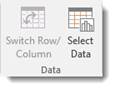
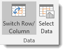
The chart in the example compares each salesperson’s monthly sales to his or her other months’ sales; however, you can change what is being compared. Just click the Switch Row/Column Data command, which will rotate the data displayed on the x and y axes. To return to the original view, click the Switch Row/Column command again.
To change chart layout:
- Select the Design tab.
- Locate the Chart Layouts group.
- Click the More arrow to view all of your layout options.
- Left-click a layout to select it.
If your new layout includes chart titles, axes, or legend labels, just insert your cursor into the text and begin typing to add your own text.
To change chart style:
- Select the Design tab.
- Locate the Chart Style group.
- Click the More arrow to view all of your style options.
- Left-click a style to select it.
To move the chart to a different worksheet:
- Select the Design tab.
- Click the Move Chart command. A dialog box appears. The current location of the chart is selected.
- Select the desired location for the chart (i.e., choose an existing worksheet, or select New Sheet and name it).
Challenge!
Use the Company Sales workbook or any other workbook to complete this challenge.
- Use worksheet data to create a chart.
- Change the chart layout.
- Apply a chart style.
- Move the chart to a separate worksheet.
Источник
Subjects>Electronics>Computers

Wiki User
∙ 13y ago
Best Answer
![]() Copy
Copy
In Excel 2007, you will find the chart commands on the Insert
tab on the menu ribbon in the charts section.
Wiki User
∙ 13y ago
This answer is:
![]()
Study guides
Add your answer:
![]() Earn +
Earn +
20
pts
Q: Where are the chart commands located Excel?
Write your answer…
Submit
Still have questions?
![]()
![]()
Related questions
People also asked
Creating and Editing Beautiful Charts and Diagrams in Excel 2019

The greatest benefit of Excel 2019 compared to other Microsoft Office software is its ability to quickly generate charts, graphs and diagrams. After you enter data into your spreadsheet, adding a chart to your worksheet is as simple as clicking a few buttons, formatting the chart, and clicking the save button. You have several options for the type of chart that you want to add to your spreadsheet, and you can even add effects and 3D elements.
Set Up Your Data
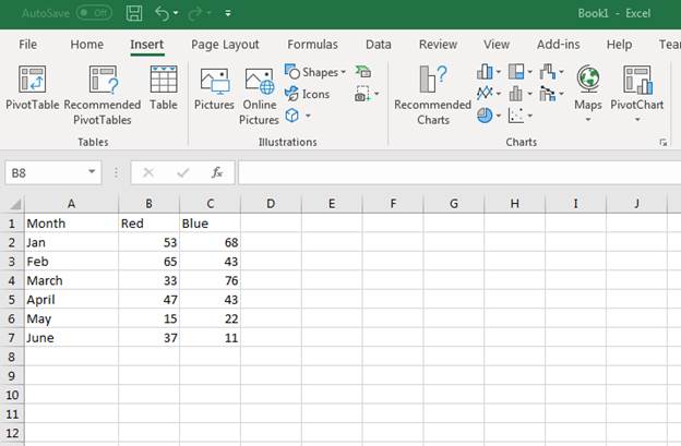
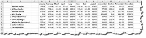
Before you can create a chart, you need some data stored in a spreadsheet. This can be test data or data from a previous spreadsheet. For this article’s examples, we’ll use a chart of products sold. The scenario is an ecommerce store that sells red and blue widgets. The following spreadsheet shows the sample data setup:
(Sample data for a new chart)
Notice that the «A» column is used for the first six months of the year. Column «B» has the number of sales for Red widgets by month. Column «C» has the number of Blue widgets sold by month. Suppose we want to see a graph to visually represent the number of sales each month. This can be done by inserting an Excel 2019 chart into the spreadsheet that contains the data.
Inserting a Standard Chart
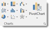
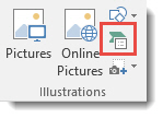
Any chart or diagram that you want to make can be found in the «Insert» tab on Excel.
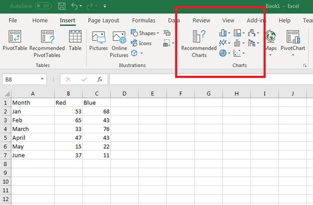
(Location of chart buttons)
Each type of chart is shown using an icon on the button. With Excel, you can make bar, line, pie, scatter, hierarchy and several others. You might be wondering which type of chart is the best for your data, and Excel has a new «Recommended Charts» function that makes a suggestion for you based on the data stored.
When you select the data for your chart, make sure that you select the row and column header cells. Excel will use these headers for the labels inserted into your chart’s image. Select cells A1 to C7 to select all data. Next, click the «Recommended Charts» button. A new window displays showing a list of recommended charts for the data selected.
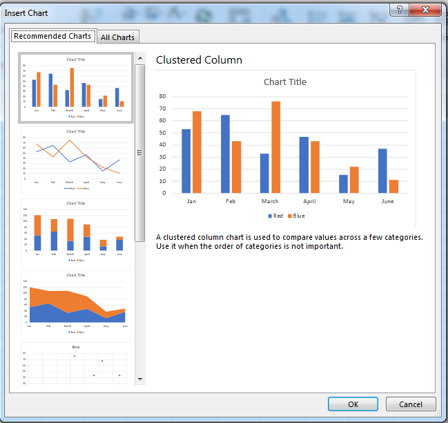
(Recommended chart window)
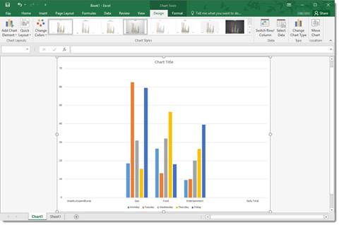
The recommendations Excel displays use column and row headers, and then add data to show you a visual representation of the chart that you’re about to insert into the spreadsheet. In the image above, Excel shows you several charts to choose from. For this example, a clustered column chart (the first option in the image above) is chosen. Excel automatically draws the chart and inserts it into the spreadsheet.
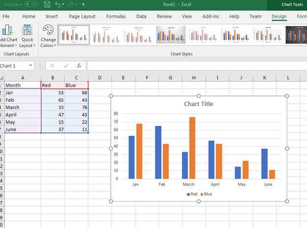
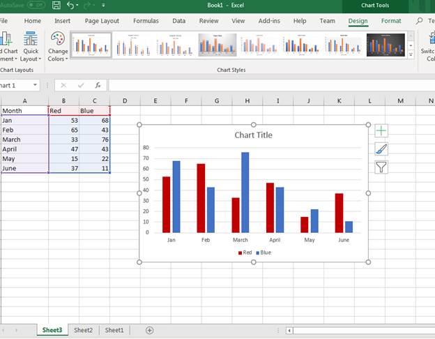
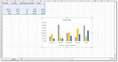
(Inserted clustered column chart)
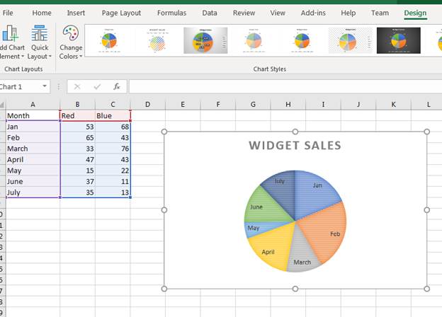
A clustered chart makes a comparison of sales for each widget based on the months of the year. For instance, in January 53 red widgets were sold and 68 blue widgets were sold. The red widget sales numbers are shown in blue, and the blue widget sales are shown in yellow.
It doesn’t make sense to display red widgets in blue, so we want to change the colors used in the bar graphs. Excel provides formatting option for charts where you can change labels, colors and even change the chart type on the fly.
To change a bar’s color, click it in the chart. A window on the right displays a list of formatting and effects that you can add to the selected component in the chart.
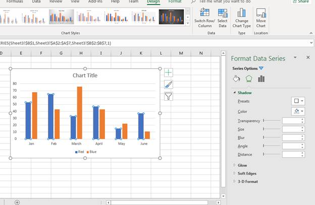
(Bar chart effects and color options)
You’ll see in the format window that you have several options. The paint bucket icons is the «Fill» button that lets you change colors and the type of pattern displayed in the selected bar (in this scenario it’s the blue bars). Click the paint bucket icon, and then click the drop down next to the «Color» label.
With the red widget sales bar shown as red, the orange bar should be a new color. We can change the blue sales bar to blue, and then the bar chart is more intuitive. After you change colors and formatting in a chart, Excel automatically changes any labels associated with a chart component.
(New chart colors updated in a sales chart)
To the left of the chart, you can see the data highlighted letting you know what Excel is using in the chart. Purple is the bar labels and the blue highlighted data is used to populate bar values. The red highlighted cells are the color labels at the bottom of the chart.
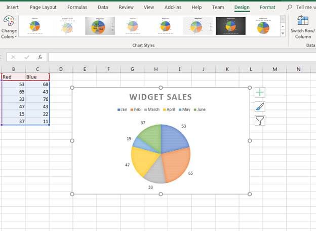
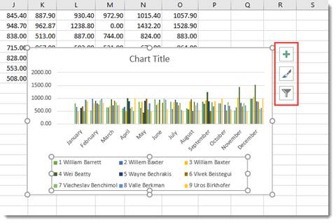
Since the spreadsheet chart has no title, Excel doesn’t know what value to give the chart title component. The default chart title is labeled «Chart Title.» You can change the chart title component by double clicking the text box. Type a new chart name for the title. In this example, the chart title was changed to «Widget Sales.»
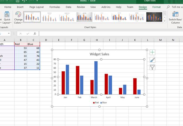
(Title change in a sales chart)
Changing a Chart’s Design
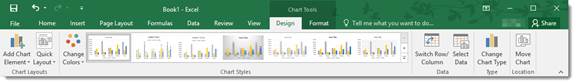
The «Format» tab displayed as an option for each image that you added to a spreadsheet. When you add a chart to a spreadsheet, the «Design» tab displays as an option. You can change several elements of a chart including the type of chart that displays in the «Design» tab. The tab is displayed by default when you first create a chart, but you need to select the tab after you’ve finished adding effects.
You have several options in the «Design» tab.
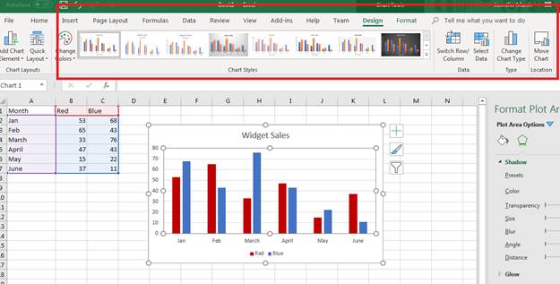
(Design tab options for a chart)
The «Chart Styles» section is where you can change the type of bar chart. Click any one of these bar chart types to change the way it displays in Excel. The downside of using this option is that Excel reverts color and effect changes back to the default. After you change the bar chart type, you again need to redo color changes and any special effects such as shadows, glow effects and 3D formatting.
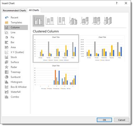
You can also change the entire chart type and switch to a new one using the «Change Chart Type» button. This button is in the «Type» section to the right of the «Chart Styles» section. Click this button and a new «Change Chart Type» window displays.
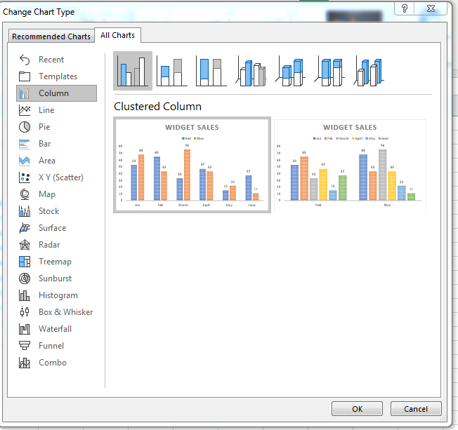
(Change Chart Type options)
Since we only used the recommended chart type function, the complete list of chart type options wasn’t initially displayed during the first chart creation. When you have a full list of chart types, you can see that Excel has several types that you can choose from. Excel orders chart types by the most commonly used, so the first few are what you’ll likely use in your own spreadsheets.
In this example, we’ll switch the chart type to a pie chart. Click the «Pie» option in the left panel. You can then choose a sub-type at the top of the window. In the image above, notice that there are several bar types. You can choose sub-types in any chart selection to make your charts visually appealing.
(A bar chart changed to a pie chart)
With a chart changed to a new type, you can still have access to the «Design» tab to make more revisions. Notice that the pie chart also changes to the default colors created by Excel. You can click any part of the pie chart to change its effects just like you did with the bar chart and the formatting window opens.
If you want to change the sub-type for a chart, you can use the «Quick Layout» button that displays a dropdown of options.
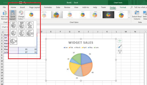
(Quick Layout options to change the chart sub-type)
The dropdown displays the sub-type options that display data in different ways for a pie chart. For instance, you can show the values within the colored areas versus the default layout that shows values outside of the colored sections. You can show a percentage indicated by the icon that shows a percent section in the icon. This feature of Excel 2019 makes it much faster and easier when choosing a new sub-type for your charts.
Click one of the options in the dropdown to change the bar chart to a different layout. Notice that the right of the chart image has several buttons. You can use these to quickly change the way a chart displays visually to users. With Excel, you have several options to pick and choose the way your charts and graphs display. You can match colors to brands or change them based on the data being used. These options along with the ease of how you can create charts is what makes Excel a great option for creating spreadsheets.
Changing Chart Data
As you continue to develop your spreadsheet, you might add more data to your chart. For instance, you might add another month to your chart. It could be August and now you want data shown from the month of July. You can change data in a chart using the «Select Data» option.
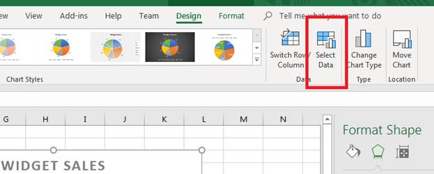
(Select Data button)
By clicking the «Select Data» button, a window opens that asks for new data. We’ve added a new row with data that reflects the number of sales in July. We now want to add this data to the pie chart.
Click the «Select Data» button and a new window opens.
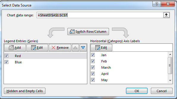
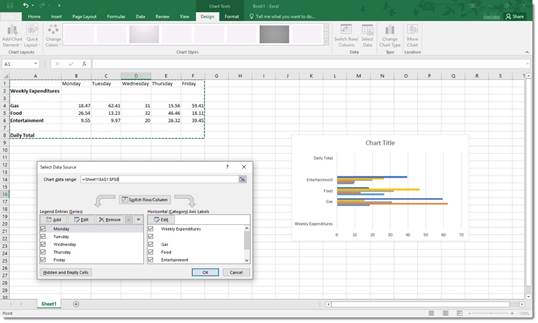
(The «Select Data» window provides options to change data used in a chart)
Notice that you can switch columns and rows. This option is beneficial when you need to change the way a chart uses data when it doesn’t translate well during chart propagation. The arrow button next to the «Chart data range» text box opens a new window that lets you choose a new range of cells for chart values. Use this to select the newly added July row stored in the spreadsheet data.
Press «Enter» when you are done with your selection, and then click «OK» to add the new range to your pie chart. Excel automatically updates the graph and displays the new results.
(Updated chart data)
Use Excel’s chart options to create graphs that represent your data in a visual format. Excel has several chart options, so any diagram or layout that you think best represents your information is available. After you create a chart, you don’t have to stick to the data chosen. You can choose new data and update it continuously as you add more information to your spreadsheet.
Remember that any changes that you don’t like can be immediately changed using the «Undo» button in the quickbar at the top of your Excel window.
Chart Recommendations
In prior versions of Excel, you had the Chart Wizard to help you create charts. That was a great tool and a great help, but Excel offers you something even better: Recommended Charts tool. This is under the Insert tab on the Ribbon in the Charts group (as pictured above).
To create a chart this way, first select the data that you want to put into a chart. Include labels and data.
When you click on the Recommended Charts button, a dialogue box opens like the one pictured below.
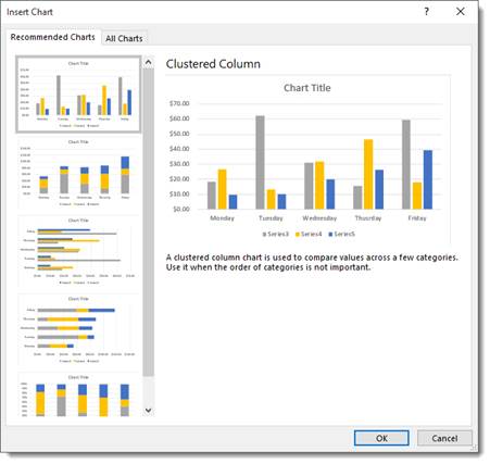
Based on your data, Excel recommends a chart for you to use.
On the left side of this dialogue box is all the chart recommendations.
On the right is a preview of what the chart will look like with your data.
Choose the chart that you want to use, then click OK.
The chart is embedded in your worksheet for you:
You’ll also notice that the Chart Tools Format tab opens in the Ribbon:
The tools shown above will help you customize your charts
Types of Charts
To the right of the Recommended Charts button on the ribbon, you’ll see this:
You can use these buttons and their dropdown menus to create these types and styles of charts. We’re going to go from left to right, starting at the top left, and cover all the buttons above.
Insert Column or Bar Chart. This is the first button, located in the top left corner. With this, you can preview data as a 2-D or 3-D vertical column chart or as a 2-D or 3-D horizontal bar chart.
Insert Hierarchy Chart. Use this chart to compare a part to a whole or to show the hierarchy of several columns or categories.
Insert Waterfall or Stock Chart. The waterfall chart is used to show how a starting value is affected by a series of positive and negative values, while the stock chart is used to show the trend of a stock’s value over time.
Insert Line or Area Chart. This lets you preview data as a 2-D or 3-D line or area chart.
Insert Statistic Chart. Use these charts to show a statistical analysis of your data. Chart types include Histogram, Pareto, and Box and Whisker charts.
Insert Combo Chart. These charts are best when you have mixed data or want to emphasize different types of information. You can preview your data as a 2-D combo clustered column and line chart – or clustered column and stacked area chart.
Insert Pie or Doughnut Chart. You can preview data as a 2-D or 3-D pie or 2-D doughnut chart.
Insert Scatter (X,Y) or Bubble Chart. Preview data as a 2-D scatter or bubble chart.
Insert Surface, or Radar Chart. With this, you can preview data as a 2-D stock chart that uses typical stock symbols, a 2-D or 3-D surface chart, or even a 3-D radar chart.
More Chart Types
Excel brings with it some new chart types to help you better illustrate data that you include in your worksheets.
These chart types include:
- Treemap. A treemap chart displays hierarchically structured data. The data appears as rectangles that contain other rectangles. A set of rectangles on the save level in the hierarchy equal a column or an expression. Individual rectangles on the same level equal a category in a column. For example, a rectangle that represents a state may contain other rectangles that represent cities in that state.
- Waterfall. As explained by Microsoft, «Waterfall charts are ideal for showing how you have arrived at a net value, by breaking down the cumulative effect of positive and negative contributions. This is very helpful for many different scenarios, from visualizing financial statements to navigating data about population, births and deaths».
- Pareto. A Pareto chart contains both bars and a line graph. Individual values are represented by bars. The cumulative total is represented by the line.
- Histogram. A histogram chart displays numerical data in bins. The bins are represented by bars. It’s used for continuous data.
- Box and Whisker. A Box and Whisker chart, as explained by Microsoft, is «A box and whisker chart shows distribution of data into quartiles, highlighting the mean and outliers. The boxes may have lines extending vertically called ‘whiskers’. These lines indicate variability outside the upper and lower quartiles, and any point outside those lines or whiskers is considered an outlier.»
- Sunburst. A sunburst chart is a pie chart that shows relational datasets. The inner rings of the chart relate to the outer rings. It’s a hierarchal chart with the inner rings at the top of the hierarchy.
Creating Charts Using the Ribbon
By using the chart options we discussed in the last section, we can quickly and easily create a chart, then embed it into our worksheet.
Let’s insert a bar chart into our worksheet below.
Start out by selecting the data you want to use in the chart.
Now click the Insert Column or Bar Chart button on the Ribbon.
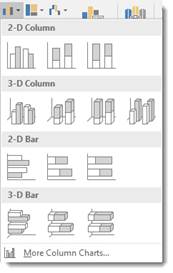
Choose the bar chart you want to use, or click More Column Charts.
If you click More Column Charts, this is what you’ll see:
On the right side of the window, you will see a list of different chart types. Click Bar.
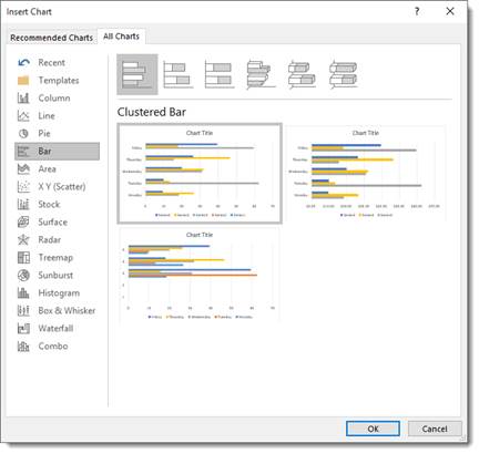
At the top, you’ll see bar charts illustrated in gray. These are different styles of bar charts. You can click on any of the styles and see a preview of your data in that style of chart (in color) in the box below.
Select the type of chart you want, then click OK.
Excel embeds the chart in your worksheet for you:
Creating a Chart from Scratch
So far in this article, we’ve taught you how to create charts by selecting your data first. However, you don’t have to do it that way (although it’s the easiest). In other words, you can start to create your chart without selecting data first.
Let’s learn how.
Click the Insert Column or Bar Chart button on the Ribbon again. However, this time, don’t select any data before you do it.
Select the type of bar chart that you want to use.
You’ll see a blank area on your worksheet where your chart will be embedded, and you’ll also notice the Chart Design and the Chart Format tabs open on the Ribbon.
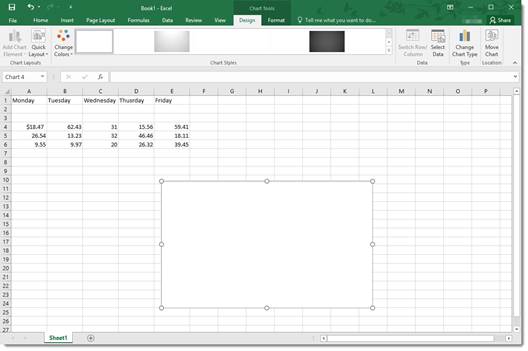
Click the Select Data button under the Design tab.
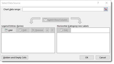
The Select Data Source dialog window will open.
The data range refers to the number of cells you’d like to use. For instance, «=Sheet1!$A$1:$G$8» refers to cells A1 through G8 on worksheet one.
It’s actually much easier to select the data range by dragging your mouse over it. To do that, click the Data Range button  next to the text box.
You’ll see another box that looks like this:
This window is simply asking you to define the data range, and you can do it easily by clicking on a cell, holding the mouse button, and dragging it over all of the cells you’d like to add. MS Excel automatically enters the selected cell coordinates into the data range window. When you are finished, you can either click the button on the right  or push Enter.
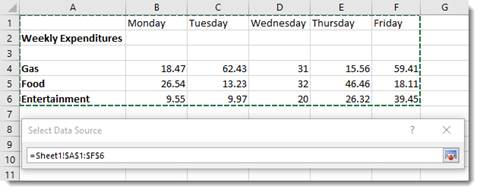
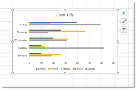
When you hit Enter, the chart appears in your worksheet:
Now you can use the Select Data Source dialogue box to add legend entries – or edit and remove them.
You can also edit your axis labels.
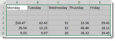
Note that your axis labels were your row labels. These appear as colors representing each day of the week.
Your legend entries were your column labels. These appear on the left, vertically.
Your data appears as the bars.
If you want, you can switch rows and columns so that the days of the week appear on the left and your axis labels become legend entries.
Uncheck any entries that you don’t want to appear in the chart.
Click OK when you’re finished.
Creating Charts Using the Quick Analysis Tool
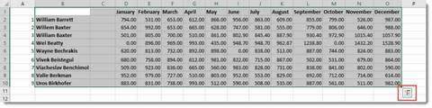
To use the Quick Analysis tool for creating charts, select that data that you want to include in chart. Click on the Quick Analysis tool button at the bottom right of the selected data (circled in red below):
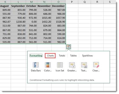
Click Charts (circled in red):
Select the type of chart you want.
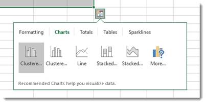
We’re going to choose a clustered chart.
The chart is embedded in your spreadsheet:
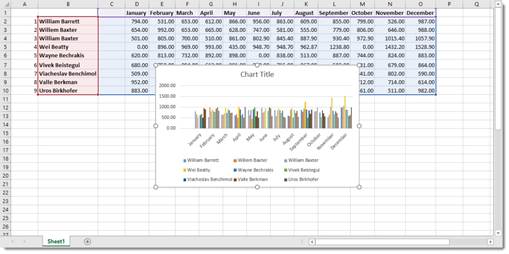
Modifying and Moving a Chart
There are a number of ways to modify a chart after it’s made.
You can right click on the plot area as we’ve done below.
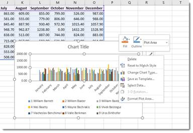
From the menu, you can delete the chart, reset, change the chart type, save the chart as a template, or select data to include in the chart. You can also format the chart area.
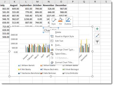
You can also click on the chart’s title to change or format it.
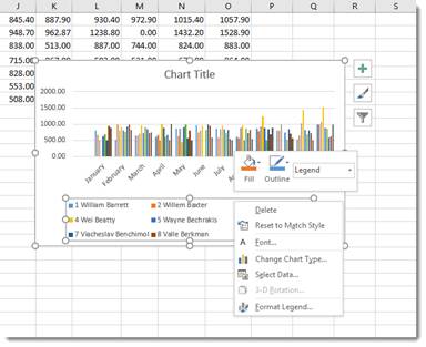
You can also right click on the legend or any other aspect of the chart to move it around and make changes. We’re going to talk about modifying chart elements in another section.
If you want to move a chart, simply click and drag any of its bounding box borders:
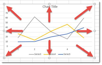
You can use the handles on the bounding box (the little circles indicated by the arrows above) to resize your chart. Drag it in to make it smaller, out to make it larger.
Chart Sheets
If you want a chart to appear on its own sheet in the workbook, simply click somewhere in the plot of the chart or select the data in your spreadsheet. Hit F11 on your keyboard.
The chart is moved to its own sheet as a clustered column chart.
Note that the sheet is named Chart1 by default. You can change that name the same way that you change any other worksheet name.
The Design Tab and Customizing Charts
The tools on the Design tab help you to customize your charts so that you achieve the look, feel, and purpose that you want.
The Design tab is pictured below. You can mouse over any tools to learn their names.

We’re going to cover all the aspects of the Design tab, starting with groups and breaking them down into tools.
Chart Layouts is the first group on the left. It contains the Add Chart Element tool and the Quick Layout tool. The Add Chart Element tool allows you to modify some elements, such as titles, data labels, legend, etc. The Quick Layout tool allows you to select a new layout for your chart.
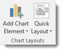
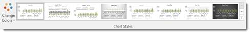
Chart Styles gives you different styles of charts to choose from. You can also change the colors used in your charts using the Change Colors tool.
The Data group allows you to reverse rows and columns in your chart. We also talked about doing this earlier. It also gives you the Select Data tool, which we used in a prior section.
The Type group contains Change Chart Type. You can change the type of chart by using this tool.
The Location group has the Move Chart tool that allows you to move the chart to a different place within your worksheet – or to another worksheet.
Customizing Chart Elements with the Chart Elements Button
The Chart Elements button appears as a plus sign whenever your chart is selected.
In the snapshot below, you can see it to the right of our chart.
When you click it, you’ll see a list of chart elements that you can add to your chart.
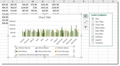
The elements that are in your chart have checkmarks beside them. You can uncheck them to remove the elements. To add an element, simply put a checkmark in the box beside it.
If you want to remove or add just a part of an element, or specify its layout as with Data Labels, you’ll use the Chart Elements continuation menu.
Here’s how to do this.
Start by putting a checkmark beside Data Labels (as an example).
You’ll see an arrow appear to the right of the word Data Labels (indicated in red below.)
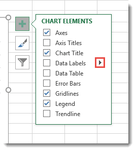
Click the arrow and you’ll see the continuation menu.
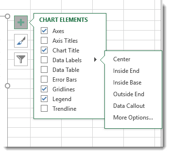
Select a layout option.
We’re going to choose Data Callout.
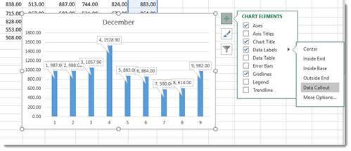
Formatting a Chart
To format a chart, you can double click in the plot area or the chart area. If you double click in the chart area, it opens the Format Chart Area pane on the right side of your window. If you double click in the plot area, it opens the Format Plot area on the right side of your screen, as shown below.
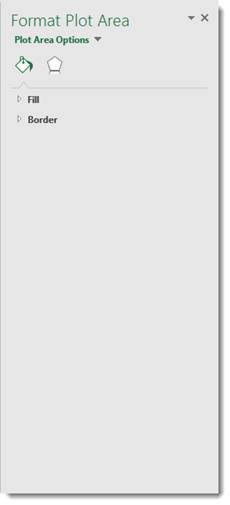
At the top of the pane, are the options.

Fill & Line looks like a bucket pouring green paint and allows you to format the fill and lines of your chart.
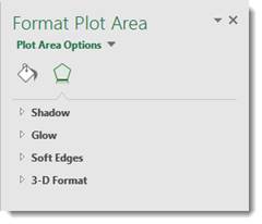
The Effects button is the one on the right, which allows you to add special effects to your chart to customize the look.
Take time to play around with the different formatting options for your charts. It’s a lot of fun to do, and you will discover interesting combinations of effects that will produce charts you’ll love.
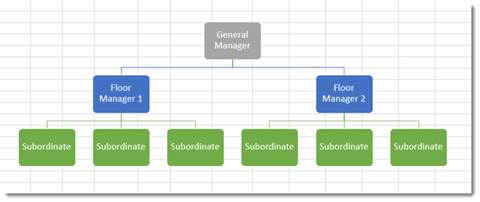
Organizational Charts or Diagrams with SmartArt
While an ordinary chart simply represents data, diagrams and organizational charts explain the causal relationship between elements. The following organizational chart, for instance, explains the relationship between managers and subordinates.
The simplest way to create an organizational chart is to click the Insert tab, then SmartArt. The SmartArt icon has been scaled down in Excel 2019, so we’ve circled it in red below.
The SmartArt dialogue box appears:
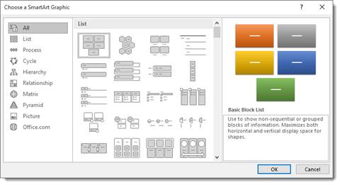
Choose the type of organizational chart or diagram you want on the left. You can choose a style from the middle section called List.
Once you choose your chart or diagram, click OK.
It appears in your spreadsheet:
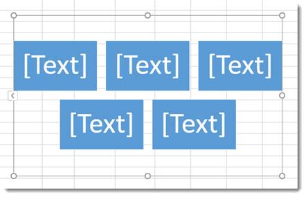
Click on the areas marked text to add your own.
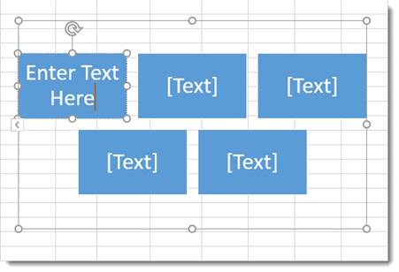
In the Ribbon, the SmartArt Design and Format tabs appear.
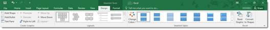
You can use these tools to change the layout, apply a style, change the colors, and other formatting elements.
View Animation in Charts
One of the debated new features in Excel 2019 is the animation added to charts.
Here’s how the animation works.
After you create a chart, then change the data for the chart in the spreadsheet, you can watch your chart and see it change too – in full animation.
In other words, if you have a bar chart, and you change the data so that a bar will be shorter, you can watch the bar slowly become shorter right after you change the data.
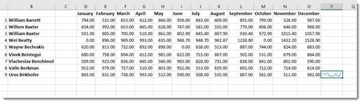
Sparklines
A sparkline is simply a small chart that’s aligned with a row of your data. It typically shows trend information.
Let’s learn how to add one in the spreadsheet below:
To insert a sparkline, go to the Ribbon, click the Insert tab, then the Sparklines group.
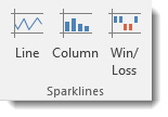
Choose the type of sparkline you want to add.
We’re going to choose Line.
You’ll see this dialogue box.
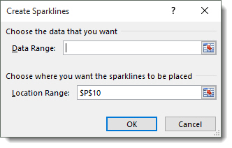
Select the cells in your spreadsheet that you want to use for your sparkline. Just drag your mouse to select the cells.
Next, enter the absolute reference for the cell where you want the sparkline to appear.
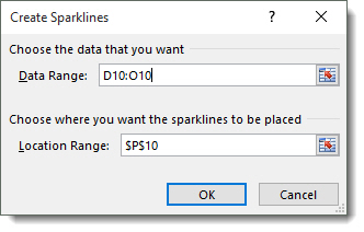
Click OK.
The sparkline now appears in the location you specified.
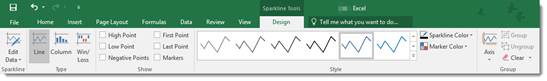
You can also format your sparkline using the Sparkline Tools Design tab that opens in the Ribbon.
A picture is worth of thousand words; a chart is worth of thousand sets of data. In this tutorial, we are going to learn how we can use graph in Excel to visualize our data.
What is a chart?
A chart is a visual representative of data in both columns and rows. Charts are usually used to analyse trends and patterns in data sets. Let’s say you have been recording the sales figures in Excel for the past three years. Using charts, you can easily tell which year had the most sales and which year had the least. You can also draw charts to compare set targets against actual achievements.
We will use the following data for this tutorial.
Note: we will be using Excel 2013. If you have a lower version, then some of the more advanced features may not be available to you.
| Item | 2012 | 2013 | 2014 | 2015 |
|---|---|---|---|---|
| Desktop Computers | 20 | 12 | 13 | 12 |
| Laptops | 34 | 45 | 40 | 39 |
| Monitors | 12 | 10 | 17 | 15 |
| Printers | 78 | 13 | 90 | 14 |
Different scenarios require different types of charts. Towards this end, Excel provides a number of chart types that you can work with. The type of chart that you choose depends on the type of data that you want to visualize. To help simplify things for the users, Excel 2013 and above has an option that analyses your data and makes a recommendation of the chart type that you should use.
The following table shows some of the most commonly used Excel charts and when you should consider using them.
| S/N | CHART TYPE | WHEN SHOULD I USE IT? | EXAMPLE |
|---|---|---|---|
| 1 | Pie Chart | When you want to quantify items and show them as percentages. |
|
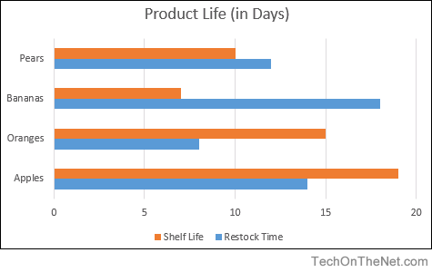
| 2 | Bar Chart | When you want to compare values across a few categories. The values run horizontally |
|
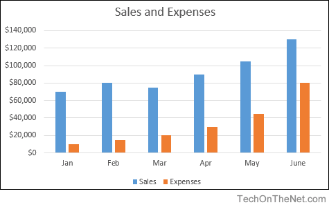
| 3 | Column chart | When you want to compare values across a few categories. The values run vertically |
|
| 4 | Line chart | When you want to visualize trends over a period of time i.e. months, days, years, etc. |
|
| 5 | Combo Chart | When you want to highlight different types of information |
|


The importance of charts
- Allows you to visualize data graphically
- It’s easier to analyse trends and patterns using charts in MS Excel
- Easy to interpret compared to data in cells
Step by step example of creating charts in Excel
In this tutorial, we are going to plot a simple column chart in Excel that will display the sold quantities against the sales year. Below are the steps to create chart in MS Excel:
- Open Excel
- Enter the data from the sample data table above
- Your workbook should now look as follows

To get the desired chart you have to follow the following steps

- Select the data you want to represent in graph
- Click on INSERT tab from the ribbon
- Click on the Column chart drop down button
- Select the chart type you want
You should be able to see the following chart

Tutorial Exercise
When you select the chart, the ribbon activates the following tab

Try to apply the different chart styles, and other options presented in your chart.
Download the above Excel Template
Summary
Charts are a powerful way of graphically visualizing your data. Excel has many types of charts that you can use depending on your needs.
Conditional formatting is also another power formatting feature of Excel that helps us easily see the data that meets a specified condition

In Microsoft Excel, a chart is often called a graph. It is a visual representation of data from a worksheet that can bring more understanding to the data than just looking at the numbers.
A chart is a powerful tool that allows you to visually display data in a variety of different chart formats such as Bar, Column, Pie, Line, Area, Doughnut, Scatter, Surface, or Radar charts. With Excel, it is easy to create a chart.
Here are some of the types of charts that you can create in Excel.
Bar Chart
- How to create a bar chart in Excel 2016 | 2010 | 2007
Column Chart
- How to create a column chart in Excel 2016 | 2010 | 2007
Pie Chart
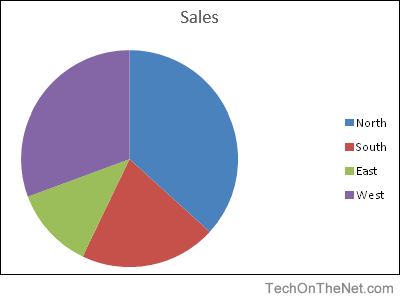
- How to create a pie chart in Excel 2016 | Excel 2007
Line Chart
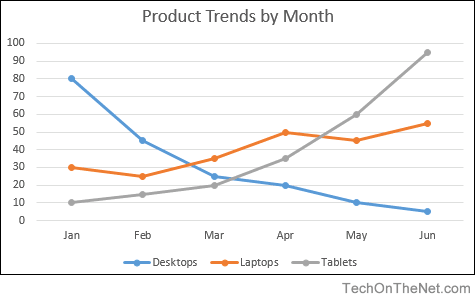
- How to create a line chart in Excel 2016 | Excel 2007
Advanced Charting
- Create a column/line chart with 8 columns and 1 line in Excel 2003
- Create a chart with two Y-axes and one shared X-axis in Excel 2007