
Every modern PC user, at least oncefaced with a package of programs Microsoft Office, which is now one of the most common, knows that it necessarily contains an application MS Excel. Now we will consider the basic concept of spreadsheets. In passing, brief information about the main elements of the structure of table elements and data and some of their possibilities will be given.
What is an Excel spreadsheet?
The first mention of the Excel program dates back to 1987, when Microsoft released its most famous office suite of applications and programs, united by the common name MS Office.

In fact, the Excel spreadsheet representsa universal means of processing mathematical data of all varieties and levels of complexity. This includes mathematics, algebra, geometry, trigonometry, working with matrices, mathematical analysis, solving complex systems of equations, and much more. Practically everything that belongs to the exact sciences of this plan is presented in the program itself. The functions of spreadsheets are such that many users not only do not know about them, they do not even suspect how powerful this software product is. But first things first.
Getting Started with Spreadsheets
Once the user opens the programExcel, he sees in front of him a table created from the so-called default template. The main working area consists of columns and rows, the intersection of which forms cells. In the understanding of working with all types of data, the main element of the spreadsheet is a cell, because it is in it that they are entered.

Each cell has a numbering consisting ofordinal designation of a column and a row, however, it may differ in different versions of the application. For example, in the 2003 version, the very first cell located at the intersection of column «A» and line «1» is designated as «A1». In the 2010 version, this approach was changed. Here the designation is represented as serial numbers and numbers, but in the description line the columns are designated as «C», and the lines as «R». Many people do not understand why this is so. But here everything is simple: «R» is the first letter of the English word row (row, row), and «C» is the first letter of the word column (column).
Used data
Speaking about the fact that the main element of the electronicThe table is a cell, you need to understand that it concerns exclusively input data (values, text, formulas, functional dependencies, etc.). The data in the cells can have a different format. The function of changing the format of the cell can be called from the context menu when the PCM is clicked on (right-click).

Data can be presented in text,numeric, percentage, exponential, monetary (currency), fractional and time formats, as well as in the form of a date. In addition, you can specify additional parameters for a kind or decimal places when using numbers.
Main window of the program: structure
If you look closely at the main windowyou can see that in the standard version, the table can contain 256 columns and 65536 rows. The bottom of the tabs are tabs. There are three of them in the new file, but you can ask more. If you consider that the main element of the spreadsheet is a sheet, this concept must be attributed to the content on different sheets of different data that can be used crosswise when specifying the appropriate formulas and functions.

Such operations are most applicable when creatingsummary tables, reports or complex computation systems. Separately, it should be said that if there are interlinked data on different sheets, the result is automatically calculated without changing the dependent cells and sheets without reintroducing a formula or function expressing this or that dependence of the variables and constants.
On top is a standard panel withseveral main menus, and just below the formula line. Speaking about the data contained in the cells, we can say that the main element of the spreadsheet is this element, because the line itself displays either text or numeric data entered into cells, or the formulas and functional dependencies. In the sense of displaying information, the formula string and the cell are the same. True, for a string, formatting or specifying a data type is not applicable. This is exclusively a viewer and input.
Formulas in Excel spreadsheets
As for the formulas, they are sufficient in the programa lot of. Some of them are unknown to many users in general. Of course, to understand all of them, you can carefully read the same reference manual, but the program also provides a special opportunity for automation of the process.

When you click on the button «fx«(Or the sign»=«) A list will be displayed, from which you can select the necessary action, which will save the user from manually entering the formula.

There is one more frequently used remedy. This is an auto-sum function, represented as a button on the toolbar. Here, too, the formula will not be introduced. It is enough to activate the cell in the row and column after the selected range, where it is supposed to be calculated, and click on the button. And this is not the only example.
Interconnected data, sheets, files and cross-references
With regard to interlinked links,the cell and the sheet can be attached data from another location in this document, a third-party file, data from some Internet resource, or an executable script. This allows you to even save disk space and reduce the original size of the document itself. Naturally, how to create such interrelations, it is necessary to understand carefully. But, as they say, there would be a desire.
Add-ins, diagrams and graphs
In terms of additional tools andMS Excel spreadsheets provide the user with a wide choice. Not to mention the specific add-ons or executable Java or Visual Basic scripts, let’s dwell on creating graphical visual tools for viewing the analysis results.
It is clear that drawing a diagram or buildinga graph based on a huge amount of dependent data manually, and then inserting such a graphic object into a table as a separate file or an attached image is not something everyone wants.

That is why their automaticcreation with a preliminary choice of type and type. It is clear that they are based on a certain data area. Just in the construction of graphs and diagrams, it can be argued that the main element of the spreadsheet is a selected area or several areas on different sheets or in different attached files, from which the values of variables and dependent computational results will be taken.
Applying filters
In some cases, it may be necessaryThe use of special filters that are installed on one or more columns. In the simplest form, it helps to search for data, text or values in the entire column. On coincidence, all the results found will be shown separately.

If there are dependencies, together withthe filtered data of one column will show the remaining values located in the other columns and rows. But this is the simplest example, because each user filter has its own submenu with certain search criteria or a specific setting.
Conclusion
Of course, consider in one article allthe possibilities of MS Excel are simply impossible. At least here you can understand what elements are the main ones in the tables, based on each specific case or situation, and also at least a little understanding, so to speak, with the basics of work in this unique program. But to fully master it will have to work hard. Often, and the developers themselves do not always know what their offspring are capable of.
</ p>>
Every modern PC user who has ever faced with the Microsoft Office software package, which is one of the most common today, knows that there is an MS Excel application in it. Now we will consider the basic concept of spreadsheets. In passing, brief information about the main elements of the structure of table elements and data and some of their capabilities will be given.
What is an Excel spreadsheet?
The first mention of the Excel program dates back to 1987, when Microsoft released its most famous office suite of programs and applications, united by the common name MS Office.
In fact, the Excel spreadsheet is a universal tool for processing mathematical data of all varieties and levels of complexity. This includes mathematics and algebra, and geometry, and trigonometry, and working with matrices, and mathematical analysis, and the solution of the most complex systems of equations, and much more. Practically everything that belongs to the exact sciences of this plan is presented in the program itself. The functions of spreadsheets are such that many users not only do not know about them, they do not even suspect how powerful this software product is. But first things first.
Getting Started with Spreadsheets
Once a user opens an Excel program, he sees a table created from the so-called default template. The main workspace consists of columns and rows, the intersection of which forms cells. In the understanding of working with all types of data, the main element of the spreadsheet is a cell, because it is in it that they are entered.
Each cell has a numbering consisting of an ordinal designation of a column and a row, however, it may differ in different versions of the application. For example, in the 2003 version, the very first cell, located at the intersection of column «A» and line «1», is designated as «A1». In the 2010 version, this approach was changed. Here the designation is represented in the form of ordinal numbers and numbers, but in the description line the columns are designated as «C», and the lines as «R». Many people do not understand why this is so. But here everything is simple: «R» is the first letter of the English word row (row, row), and «C» is the first letter of the word column (column).
Used data
Speaking about the fact that the basic element of the spreadsheet is a cell, it is necessary to understand that it concerns exclusively input data (values, text, formulas, functional dependencies, etc.). The data in the cells can have a different format. The function of changing the format of the cell can be called from the context menu when the PCM is clicked on (right-click).
The data can be presented in text, numeric, percentage, exponential, monetary (currency), fractional and time formats, as well as in the form of a date. In addition, you can specify additional parameters for a kind or decimal places when using numbers.
Main window of the program: structure
If you look closely at the main application window, you will notice that in the standard version, the table can contain 256 columns and 65536 rows. The bottom of the tabs are tabs. There are three of them in the new file, but you can ask more. If we assume that the main element of the spreadsheet is a sheet, this concept must be attributed to the content on different sheets of different data that can be used crosswise when specifying the appropriate formulas and functions.
Such operations are most useful when creating summary tables, reports, or complex computation systems. Separately, it should be said that if there are interlinked data on different sheets, the result is automatically calculated without changing the dependent cells and sheets without reintroducing a formula or function expressing this or that dependence of variables and constants.
On the top is a standard panel with several main menus, and just below the formula line. Speaking about the data contained in the cells, we can say that the main element of the spreadsheet is this element, because either the text or numeric data entered into the cells or the formulas and functional dependencies are displayed on the line itself . In the sense of displaying information, the formula string and the cell are the same. True, for a string, formatting or specifying a data type is not applicable. This is solely a viewer and input tool.
Formulas in Excel spreadsheets
As for the formulas, there are a lot of them in the program. Some of them are unknown to many users in general. Of course, to understand all of them, you can carefully read the same reference manual, but the program also provides a special opportunity for automation of the process.
If you click the » f x » button (or the » = » sign) on the left, a list will be displayed, from which you can select the desired action, which will save the user from manually entering the formula.
There is one more frequently used remedy. This is an auto-sum function, represented as a button on the toolbar. Here, too, the formula will not be introduced. It is enough to activate the cell in the row and column after the selected range, where it is supposed to be calculated, and click on the button. And this is not the only example.
Interconnected data, sheets, files and cross-references
As for interlinked links, data from another location in this document, a third-party file, data from some Internet resource or an executable script can be attached to any cell and sheet. This allows you to even save disk space and reduce the original size of the document itself. Naturally, with how to create such interrelations, it is necessary to understand carefully. But, as they say, there would be a desire.
Add-ins, diagrams and graphs
In terms of additional tools and capabilities, MS Excel spreadsheets provide the user with a wide choice. Not to mention specific add-ons or executable Java or Visual Basic scripts, let’s stop at creating graphical visual tools for viewing the analysis results.
It is clear that drawing a chart or building a graph based on a huge amount of dependent data manually, and then inserting such a graphical object into a table as a separate file or an attached image is not something everyone wants.
That is why their automatic creation is used with a preliminary choice of type and type. It is clear that they are based on a certain data area. Just as in the construction of graphs and diagrams, it can be argued that the main element of the spreadsheet is the selected area or several areas on different sheets or in different attached files, from which the values of variables and dependent computational results will be taken.
Applying filters
In some cases, you may need to use special filters that are installed on one or more columns. In the simplest form, it helps to search for data, text or values in the entire column. On coincidence, all the results found will be shown separately.
If there are dependencies, together with the filtered data of one column, the remaining values located in the other columns and rows will be displayed. But this is the simplest example, because each user filter has its own submenu with certain search criteria or a specific setting.
Conclusion
Of course, to consider in one article all the features of the MS Excel software package is simply impossible. At least here you can understand which elements are the main ones in the tables, based on each specific case or situation, and also at least a little understanding, so to speak, with the basics of work in this unique program. But to fully master it will have to work hard. Often, and the developers themselves do not always know what their offspring are capable of.
This article will demystify and help you walk through the basics of Excel and make your journey of how to understand Microsoft Excel a lot simpler and enjoyable. Making your basics crystal clear is essential if you want to understand the advanced functionality of Excel.
So, let’s get started with the building blocks of Excel;
A Single Spreadsheet
It is a single spreadsheet consisting of rows and columns. It is basically an element of the Excel Workbook. By default, the name of the first worksheet is “Sheet1”. So, a workbook is like an entire textbook, while a worksheet is a single page within that book.
A worksheet is in a tabular format consisting of rows and columns. Row numbers are placed vertically at the left side of the sheet and range from 1 to 1048576, whereas column headers are placed horizontally at the top of the sheet and range from A to XFD.
An intersection of a row and a column is called Cell and is identified with a combination of column headers and row numbers like A10 or C76.

Excel Workbook
In the query how to understand Microsoft excel you need to know about what an excel workbook is? It is the entire Excel file that contains one or more sheets. A simple Excel Workbook can be of a type – .xls or .xlsx. To create a new workbook, follow the steps below:
1. Open Excel and Click on File
2. Click New, Under Featured, click on Blank workbook.

Ribbon
At the top of the Excel Window, there is a strip of buttons and icons called ribbon. It helps you navigate and choose from various commands of Excel.
An Excel Ribbon has five parts – Tabs, Groups, Command, Quick Access Toolbar, and Dialog launchers. The ribbon consists of various tabs like Home, Insert, Page Layout, Formulas, Data, Review, and View. Within each tab, there are several groups of commands.
For example
Home is a tab, and within the Home Tab, there is a group called “Alignment,” and under alignment, there is a command “Wrap Text.” The fourth component – A Quick Access Toolbar, is a customizable toolbar to add the most frequently used commands.
Lastly, a dialog launcher is a small downward pointing arrow in the bottom right of each group. It is used to open a dialog box that can be used to input information and make choices about different aspects of the current worksheet or its content.

Entering Data In Excel
Now that we have covered the basic terminology used in Excel, we will shift our focus onto entering information or functions in Excel. To enter data in Excel, simply select a cell and start typing. The text will appear on the Cell as well as on the formula bar at the top.
After entering the information, press Enter to submit the data and move to the Cell below or press tab to submit the data and move to the Cell on the right. To enter data on a new line within a cell, i.e., insert a line break, press Alt + Enter.
Types of data in excel
The three main types of data are Text, Number, and Formulas.
Text is mainly used to provide headings to tables/columns, write descriptions, etc., and contain letters, numbers, special characters. It is by default aligned to the left side of the Cell. Note: To enter a numerical value or formula as a text, type an apostrophe before it.
The number is used for calculations, and these are aligned towards the right side of the Cell. This type of data includes integers, decimals, percentages, currency, accounting, etc. To enter a date in Excel, type the date in the default format mm/dd/yyyy or whichever format is selected for that Cell. To change the format, simply press Ctrl + 1, then in the dialog box, select a date and select the appropriate format. Note: Dates and Time are also stored as numbers in Excel. January 1, 1900, is stored as number 1, and January 2, 1900, is stored as number 2.
To convert a text to a number, simply select the Cell and click on the small down arrow next to “General” under Home Tab and Select “Number.” Data will be converted to data with two decimal points.

You can increase or increase the decimal points using the icons under the number section of the Home tab again.

Formulas are mathematical equations that direct Excel to perform calculations. Each formula has a specific syntax that users must follow to make that function work. It uses hard-coded numbers and values in other cells to do calculations.
Examples are =32*(12+10) or =A2*B4 or =A2*(12+C4)
* Several custom number formats can be applied to the data in Excel. Let’s look at some of the examples below:
You can convert a number to a specific currency by selecting the Cell and then click on the small arrow next to the “$” icon under the Number section in the Home tab. From the dropdown list, select the desired currency.

For further customization, press Ctrl + 1, and in the dialog box, select “Currency.” From here, you can choose the currency of the symbol dropdown list, increase or decrease the decimal point and choose the formatting to negative values. A sample of your selection will also be displayed in the box.

* To convert a number into a percentage, simply press the “%” icon under the Home tab’s Number section. This will multiply the number by 100 and add a percentage sign to the display.

* To convert a number into accounting format, simply select Accounting from the dropdown in the number section. This will add the $ sign and two decimal places.

* To apply comma style, simply press the “icon under the Number section in the Home tab. This will add commas to large numbers and two decimal places (so 1000 becomes 1,000.00).

* To convert a number to Zipcode +4, Press Ctrl + 1, and under category select “Special.” This will convert the number to the pattern 00000-0000. Other options like social security numbers and phone numbers are also available in the same dialog box.
* If you want to add units to a number, you can do that using Custom Formatting. For example, you want figures in Millions in a table, and you want the word “Million” written next to the number with a $ dollar sign. (Convert 76 to $76 Million). To do that, press Ctrl + 1 and select Custom, and in the Type field, write $General” Million.” It will make the data look like text, but they are still a number.
* To add Color to your number type, go to Custom in Format Cell dialog box. Write color name enclosed in square brackets before the number format. If the current formatting is $#,##0, to add blue color the format will now be [blue]$#,##0.
Writing A Formula In Excel
To write a formula, begin with an = or + sign and use numbers or cell references in order to indicate which values are to be used in the calculation. Follow the steps below:
· Type = or +
· Enter cell references like A12 or F8
· Enter an operator like +, -, * or /
· Enter the second cell reference. Continue if necessary
· Hit Enter
Consider an example where there is a list of sales for 12 months, and total annual sales need to be calculated. This can be done using an excel formula.
There are two ways of doing it – How to understand Microsoft excel; a thought that triggers you to find more and more.
1. Create a summation formula where you add in all the numbers by typing them. Example =1787092+2467847+…….+2359196. Even though this formula will give you a correct answer, it will not be dynamic. This formula needs to be changed each time there is a change in the set of monthly sale values.
2. Create a formula that sums the value using cell addresses. Instead of inserting the number, we will give the cell reference that contains the number. Example: =SUM(B2:B13)
With this formula, the values that are inserted in the Cell will be used for calculation, making the formula dynamic.
In this second example below, we need to calculate fixed costs per unit. We have the total fixed cost entered in cell B2 and the number of units in cell B3. The result should be displayed in cell B4.

So, we will select cell B4 and write the formula =B2/B3 to get the amount of fixed cost per unit.

After creating this formula, even if you change the value in cell B2 or B3, the result in cell B4 will be updated automatically based on the new values.
Note: You can see that even though the result, i.e., $1720, is shown in cell B4, the formula, i.e., =B2/B3 is visible on the formula bar. You can even edit the formula directly from the formula bar.
In this example, we have used the formula to perform division; we can add, subtract or multiply the same way by simply changing the plus division to an appropriate operator in the formula.
The operator follows a default order in which the calculation occurs. The order of operators is as follows:
1. Parenthesis
2. Exponential
3. Multiplication and Division
4. Addition and Subtraction
So, if we use this formula =6+7*2, Excel will first multiply seven by 2, and then the result, i.e., 14, is added to 6. The result will then be 20.
For more information on formulas, click here<<link to Excel Formulas article>>
Format Data As Table
If we have a list of the information entered in Excel and want to format it as a table, we should follow the steps below:
* Click on any cell in the table and press Ctrl + A to select the entire table.
* To apply borders, Go to Home Tab > Under Font Group, Click on Borders icon > From the dropdown Select All.

* Select the Headers of the table, and under Home Tab and Font Group, Select B (to make the header bold), fill color grey, and change the font color to white.

* Select Column F and G and change number formatting to currency. Go to Home Tab> Under Number Group > Click on the Dollar Sign > Select the appropriate currency.
Press Alt + W + V+ G to remove gridlines and your table with formatting is ready!

Formatting In Excel
The main goal of an Excel Worksheet is to make the data presentable, attractive and to be able to understand the data quickly. All this can be done using Excel formatting! The points below will guide you with the different ways of formatting the content:
* Change Font – By default, the Font is set to Calibri. To change the Font, go to Home Tab > Click on the arrow next to the Font Command > Select the appropriate Font. If you hover on the different options in the dropdown, a live preview of the same will be visible.

* Change Font Size – To change the font size, go to Home Tab > Click on the arrow next to the Font Size Command > Select the appropriate Font Size. You can click on either “Increase Font Size” or “Decrease Font Size” to change the size.

* Change Font Color – To change the font color, go to Home Tab > Click on the arrow next to the Font color Command > Select the appropriate Font color.

* Use Bold, Italics, Underline – Select the Cell where you want to apply the formatting. Press Ctrl + B to make text bold, Ctrl + I to make it italics, and Ctrl + U to make it underlined. Or else, you can simply click on “B,” “I,” or “U” symbols under Home Tab.

* Change cell color – Select Cell> Click on Home Tab > Click on the arrow next to Fill Color> Pick the Color you want. Or simply press Alt + H + H and pick the color you want.

* Apply pattern – Select cell > Click on Home Tab > Click on Format Cells dialog launcher > Under Fill Tab > Select Pattern Color and Pattern Style.

* Change Horizontal and Vertical Alignment – Select Cell > Under Home Tab > Select Top, Middle, or Bottom alignment to change vertical alignment and Select Left, Middle, or Right Alignment to change horizontal alignment.


* Apply cell style – Select the Cell> Home tab > Click on cell style > Choose the desired style from the dropdown menu. Note: Once you select a cell style, all existing formatting except text alignment will be replaced.

* Wrap Text – If the text entered in a cell cannot be fully visible in a single line, we can select the Wrap Text function from Home Tab to make the data fit properly.

* Apply Number Formats – Under Home Tab > Click on the dialog box launcher; it will open the Format Cells dialog box where a complete list of number formats is available on the Number tab. You can select the desired format from various options, including numbers, dates, times, fractions, percentages, and other numeric values.
- Note: You can press Ctrl + 1 to open the Format Cell Dialog box.
- Note: Excel will sometimes change number formats automatically based on the data entered.

* Add Borders – To add borders, select the Cell and click on the borders icon under Home Tab. Select the appropriate border line and Color.

* Format Painter – To copy-paste formatting from one cell to another, simply select the Cell with formatting and click on the format painter icon in Home Tab and then click on the Cell where you want to paste the formatting.
Note – Once you click on the format painter icon, the arrow will be replaced with the format painter icon.

* Clear Formatting – To clear formatting in a cell, Select the Cell> Go to the Home tab > Go to the Editing group > Click on the arrow next to the Clear button > Select Clear Formats.

Printing Work Sheet In Excel
Now that your data is ready, you will need to print it. So, let’s move to the process of how to print a worksheet and the print setting available in Microsoft Excel.
The following points will guide you through the same:
* To print a worksheet, click on File tab > Click on Print. In the dialog box, we will be able to see a preview of the page that will be printed, and we can click on the big Print button to start printing.
Note: At the bottom of the dialog box, click on the previous or next button to preview other pages.
* To print multiple pages, hold down CTRL + click the name of each workbook to print, and then click Print.
* To print multiple copies, increase the number of copies from 1 to the desired number. You can also select collated or uncollated option from the dropdown. Note: Collated prints all pages of the 1st copy and then 2nd and so on whereas uncollated prints all copies of 1st page, then 2nd page, etc.
")
")
* To print only the active worksheet, click on “Print Active Sheet” from the dropdown under the settings option.

* Page orientation can also be changed (landscape or portrait) from the dropdown available.

* To adjust page margins, either select from the pre-defined options (Normal, Wide, or Narrow) Or click the ‘Show Margins’ icon at the bottom right of the window. Now you can drag the lines to change the page margins manually.

* If the entire table needs to be printed on 1 page, it can be done by selecting the “Fit Sheet on One Page” option from the scaling dropdown list. Other options available are “Fit All Columns on One Page” and “Fit.

* To set a print area, select the cells you want to print > go to Page Layout > Click on Print Area > Select Set Print Area.

Save An Excel File
To save an Excel file, click the Save icon in the top left of Excel or simply press Ctrl + S. A Save As dialog box will open; on the left panel, click on “Save As.” Under Save As, you can see four items: OneDrive, This PC, Add a Place and Browse. By default, the “This PC” option is selected, and your file will be saved in “My documents.”
If you want your file to be saved in the My Documents folder, type a file name and click on Save. Otherwise, click on the “More options…” link, select the desired folder, give a file name, and click on the Save icon.
Below The File Name Box
There is a dropdown from which you can select the file type like.xlsx or. xlsm etc.
In this article, we have tried to cover the basics of what Excel can do. Excel has many functions and formulas that can help you automate your work and make you faster and more efficient in Excel.
Follow us for more articles and tutorials to understand Microsoft Excel!
Microsoft Excel is a spreadsheet program that comes packaged with the Microsoft Office family of software products. Just like the other programs by Microsoft, Excel can be used for a wide variety of purposes such as creating an address book, grocery lists, tracking expenses, creating invoices and bills, accounting, balancing checkbooks and other financial accounts, as well as any other purpose that requires a spreadsheet or table.
About Excel 2013
Excel is much more than a basic spreadsheet program. It gives you the complex tools and features you need to design professional spreadsheets, but all with just a few clicks of the mouse.
The good news is that Excel makes everything easy. By learning how to navigate the program, and where to find each feature, operating Excel can become a breeze!
You can use Excel to:
-
Organize, sort, and record data.
-
Enter in text and mathematical data.
-
Keep statistics.
-
Keep records.
-
Create mathematical equations and functions to accurately keep records, statistics, and data.
-
And much more!
Downloading Excel 2013
With the launch of Office 2013, Microsoft made changes in how they sell their most popular software package. Of course, you can download a free trial by simply going to the Microsoft Office page, picking out what version you want to try, then downloading the software. You don’t need a credit card to try the software.
If you want to purchase the software, Microsoft now gives you two choices. As always, you can buy the software — either online or from most office supply or computer stores. The prices to buy the software vary depending on what version you wish to purchase. There are three versions: Home and Student, Home and Business, and Professional. As with other versions of Office, it’s a one time charge and the software is yours to use as long as you wish.
However, with Office 2013 also comes Office 365, which is another method that you can use to buy the Office suite of software. With Office 365, you subscribe to the software instead of just purchasing it like you’ve done in the past. You can pay for your subscription by the month or year on the Microsoft Office website. The price of your subscription will be determined by the version that you want: Home, Small Business, or Mid-size Business.
Once you purchase a subscription, you’ll be able to download Office 2013 on your computer just as you would if you had bought the software in a store. As part of Office 365, you’ll also be given multiple licenses, which will give you the ability to install the software on other computers, as well. This is a perk that doesn’t come with buying the software in a store. For the Home version, you get up to five licenses (five devices). The Small Business version comes with licenses for up to 25 users. The Midsize Business provides for up to 300 users. There’s also an Enterprise version for larger companies that offers unlimited users.
Once you subscribe to Office 365, you’ll never have to worry about purchasing a new version of Office ever again. When a new version comes out, your software will be updated for you.
What’s New in Excel 2013
Excel 2013 is arguably the best version yet. It contains the same great features you loved in past versions, which have been fine tuned and improved for better usability. In addition, it contains some great new features that make Excel even more useful and functional than ever before.
Here are the improvements:
-
The new Start Screen makes getting started in Excel easier than ever. You can start a blank spreadsheet, or open a template – and get busy!
-
The new Quick Analysis tool makes it easy to convert data into a chart or table. All it takes is two steps (sometimes even less).
-
Flash Fill finishes your work for you in 2013. When Excel detects a pattern in your data, it enters the rest of the data for you.
-
Don’t know what type of chart to use? Chart recommendations now shows you the best chart for your data.
-
Improved slicers can now filter data in tables and query tables.
-
Each workbook now has its own window.
-
New functions
-
Save and share files online – for free!
-
Embed your worksheet data in a web page
-
The new Design and Format tabs make it easier to format charts and tables.
-
View animation in charts
-
And more!
Getting Started In Microsoft Excel
You open Microsoft Excel by clicking on the icon on your desktop (if you have one there) or in the program bar. The icon for Microsoft Excel 2013 looks like this:

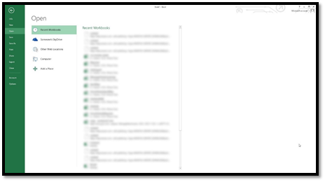
When you click on the icon, Excel 2013 will open, and you’ll see the Start Screen. This is new to 2013.
The Start Screen looks like this:
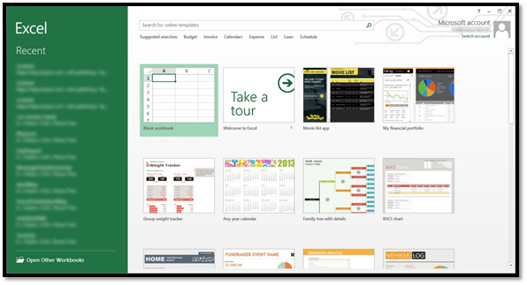
On the left, you’ll see the dark green column that contains your recently opened files. You can click on any of these to open them. To the right, you’ll see templates you can use to start a new Excel workbook. You can also choose to just open a workbook, as we’ve selected above.
Let’s open a blank spreadsheet.
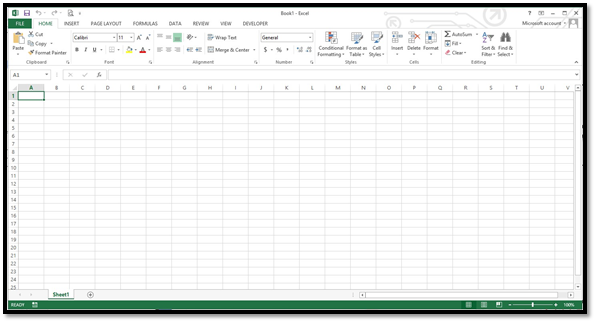
This is a new workbook for which the default name is Book1. You can see the name in the Title bar.

For each additional new workbook that you open, the name increases by one digit: Book2, Book3, etc. If you start MS Excel by clicking on an already existing workbook on your computer, it will open automatically and your workbook will be displayed in the MS Excel window.
Touring the Excel 2013 Interface
Let’s take a look at the blank workbook again. This time, however, we’ve labeled the different parts of the interface that you’ll use in Excel 2013.
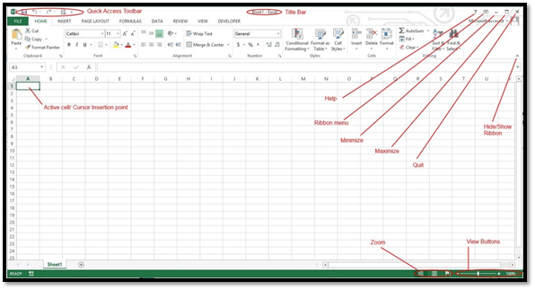
Take a few minutes to look at the features that we’ve labeled for you. It’s not important that you know how to use these things right now. For now, just take a second to familiarize yourself with where everything is located. The items labeled above help to make using Excel 2013 easier, but they’re not the bread and butter.
If you look below the Quick Access Toolbar (as labeled above), you’ll see the Ribbon. The Ribbon was first introduced in Office 2007.

The ribbon is divided into tabs. These tabs are also menus. The tabs are Home, Insert, Page Layout, Formulas, Data, Review, View, and Developer.
Below each tab are commands (or tools) you can use. The commands (or tools) located beneath each tab relate to the tab. For example, under the Page Layout tab, you would find tools to create a page layout.
That said, the tools under each tab are broken down into groups so that you can easily find what you need. In the snapshot above, we’re looking at Home. The groups within the Home tab are Clipboard, Font, Alignment, Number, Styles, Cells, and Editing. Below is a snapshot of the Alignment group.
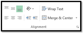
In the Alignment group are all the tools that are related to alignment.
If you look to the right of the word «Alignment,» you’ll see an arrow in the lower right corner. If you click this, it will take you to the Alignment options dialog box. You can click this arrow in any group to open the options for that group.
Working with Excel 2013 on a Tablet
If you’re using Excel on a tablet, you can adjust the spacing between buttons on the ribbon to make it easier to use. You do this by activating Touch mode.
To do this, click or touch the Quick Access Toolbar button:
Select Touch/Mouse Mode.
You can now see the button in the Quick Access Toolbar, as shown below:
Now, touch or click the button and choose Touch.
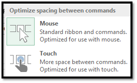
There is now more space between commands on the Ribbon.
Learning how to navigate around Excel is critical to being able to successfully use the program. In this section, we’re going to focus on the major elements of Excel 2013 and take a few minutes to become familiar with their purpose.
If you have access to Excel 2013, you should open a blank spreadsheet at this time.
Understanding the Basic Elements of an Excel Spreadsheet
Before going any further in this section, it’s important to understand the elements of a spreadsheet, in Excel, or any spreadsheet that you may use.
A spreadsheet is made up of individual cells. One cell is simply a block on your screen. In the snapshot below, you can see a cell that’s highlighted:
The cell above is highlighted because it’s an active cell. In other words, we clicked on it with our mouse to make it active so we can enter data into it.
Now, all the cells in a worksheet are organized into columns and rows. In Excel, rows are represented by numbers. Columns are represented by letters.
Below is a snapshot of row 5, followed by a snapshot of column C.

Rows are horizontal. Columns are vertical.
Since rows and columns are labeled with numbers and letters respectively, you can also locate the exact coordinates of a cell.
For example, instead of your boss coming to you and telling you the number for March’s expenses for employee Susie Smith are wrong, he can simply say, recheck the number in D15. This would tell you to go to column D, row 15.
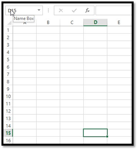
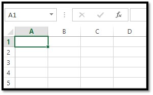
Then, instead of scrolling through your worksheet, simply go to the Name box above Column A (pictured below). In the snapshot below, you’ll see A1 highlighted in blue. This is the Name box.
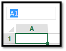
Enter the coordinates for the cell. We’re going to enter D15, then hit Enter.
As you can see below, Excel took us to the exact cell and highlighted it for us.
The Formula Bar
The formula bar is the magical ingredient of the soup, so to speak. It is what makes Excel easier to use than doing spreadsheets by hand, or using other programs where you’re left to do the math by yourself.
In this section, you’ll learn how to enter formulas and equations into MS Excel 2013. The formulas and equations that you enter will be entered in and displayed in the Formula Bar. It is located to the right of the Name Box.

The Formula Bar has the fx to the left of it.
On the left side of the Formula Bar are the Formula Bar buttons. The Insert Function button is fx. When you start making or editing a cell entry, X is Cancel and the check mark is Enter.
The white area (or bar) to the right of the buttons is the Cell Contents area. The Formula Bar always shows you the contents of a cell, even if it doesn’t appear in the cell. In other words, it shows equations in the cell even if the cell only displays the answer to the equation. It will show contents of cells that appear to be blank in the spreadsheet as well. If the Cell Contents area is blank, you know the cell is empty.
The Backstage Area
The Backstage area is located under the green File tab at the upper left hand corner of the Excel window. If you click on it, this is what you see:
Using the Backstage area, you can open an existing spreadsheet, create new spreadsheet (either blank or template), save workbooks and spreadsheets, share workbooks and spreadsheets, print, close, and set options for the Excel program.
Click the left facing arrow at the top left of the Backstage area to go back to your spreadsheet.
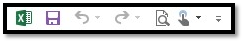
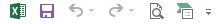
The Quick Access Toolbar
The Quick Access Toolbar is located at the top left of the Excel window. It looks like this:

You can use the Quick Access toolbar to add shortcuts to tools that you use frequently, rather than having to click tabs and find the tools in a group.
By default, our Quick Access toolbar displays these shortcuts:
 Save
Save
 Undo
Undo
 Redo
Redo
 Print Preview/Print
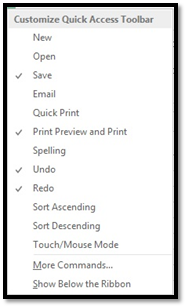
You can customize the Quick Access toolbar and add shortcuts so the tools you need appear there for easy access.
Click the drop-down menu to the right of the toolbar. It looks like this: 
Now, click on the shortcuts you want to add to the toolbar from the list. When you click on a shortcut, it will put a check mark beside it, letting you know it appears on the toolbar.
If you want to add a shortcut for a tool, but you don’t see it on the Customize Quick Access Toolbar list, you can still add it to your toolbar. You do this by adding Ribbon commands.
Simply go to the Ribbon and find the tool that you want to add. Right click on the tool (or tab and hold if you’re using a touchscreen device).
In this example, we’re going to add SmartArt under the Insert tab.
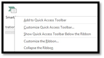
Select Add to Quick Access Toolbar.
As you can see, it’s now added:
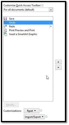
If you want to move a command button in the toolbar to a different location or group it with other buttons on the toolbar, select the Customize Quick Access Toolbar downward arrow (on the Quick Access toolbar), then select More Commands.
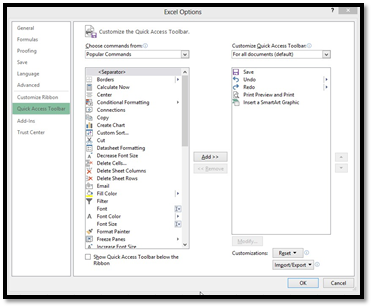
On the right side, you can see everything that’s added to the Quick Access toolbar. They are listed in the order they appear on the toolbar.
If you want to change its location, click on it to select it, then use the arrows to the right to move it up or down.
If you want to group buttons on the Quick Access toolbar, you can add vertical separators. To do this, select <Separator> from the list on the left:
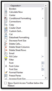
Then click the Add button twice.
To add shortcuts listed in the left column, click the shortcut to select it, then click the Add button.
To remove shortcuts from the Quick Access toolbar, select the shortcut in the right column, then click the Remove button.
Moving Around Worksheets
Being able to navigate through a worksheet will make using Excel a lot easier. However, before we discuss that, let’s quickly review three things you have to know about the worksheet area. Remember, the worksheet area contains cells, rows, and columns.
-
The cell cursor is the dark green border that appears around a cell. It means a cell is active.
-
The location of the cell, or address, appears in the Name box.
-
The cell’s row number and column letter are shaded. Look at the snapshot below. Note that the row number 1 is shaded differently than the rows after. Note that the column A is shaded differently than the other columns.
This is because cell A1 is active, as confirmed by the Name box and the green border around the cell.
Now, since the Excel worksheet contains so many cells, rows, and columns, not all of your cells are going to be displayed at once on the screen. For that reason, there are several ways that you can use your mouse cursor to move through and navigate your worksheet.
Of course, if the cell is displayed, you can simply click on it to make it active. If you’re using a touchscreen, just tap it.
You can also type the coordinates in the Name box and be taken to the cell.
Press F5 to open the Go To dialog box.
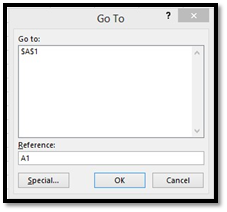
All you have to do is type the address of the cell in the Reference box (pictured above).
You can also use cursor keys to move to the desired cell. The cursor keys are displayed in the table below:
|
Keystroke |
Action |
|
Moves cell to the right |
|
? on the keyboard or Shift+Tab |
Moves cell to the left |
|
Up arrow on the keyboard |
Moves one cell up |
|
Down arrow on the keyboard |
Moves one cell down |
|
Home |
Moves cursor to cell in Column A of the current row |
|
Ctrl+Home |
Moves cursor to the first cell — A1 |
|
Ctrl+End or End, Home |
Moves the cursor to the cell that’s at the intersection of the last column with data and the last row that has data in it |
|
Page Up |
Moves the cursor to cell that’s one full screen up in the same column |
|
Page down |
One full screen down (in the same column) |
|
Ctrl+? or End, ? |
Moves the cursor to the first occupied cell that’s to the right that’s has a blank cell before it or after it. If there isn’t an occupied cell, it goes to the end of the row |
|
Ctrl+? or End, ? |
Same as above, except first occupied cell to the left. |
|
Ctrl+ Up arrow, or End, Up Arrow |
Moves the cursor to the first occupied column above that has a blank cell before it or after it. |
|
Ctrl+Down arrow, or End, Down arrow |
Same as above, except for first occupied cell below. |
|
Ctrl+Page Down |
The cursor moves to the next worksheet of the workbook |
|
Ctrl+Page Up |
Moves to the previous sheet of the workbook |
Using the Touch Keyboard
If you’re using Excel on a tablet or other touch-enabled device, you can also use the on-screen touch keyboard. Instead of entering characters (letters, numbers, and spaces) by pecking away on your keyboard, you’ll simply touch your finger or stylus pen to the keyboard on the screen.
Make sure you enable Touch mode before starting to use Excel from a tablet or touch device.
To use the on-screen keyboard, simply tap in the spreadsheet area to see the cursor – and the keyboard.
The Status Bar
The Status Bar appears at the bottom left of your Excel window. It contains the following information about your spreadsheet:
-
Mode Indicator shows the state of your Excel program, such as Ready, Edit, etc. It will also tell you if any special keys are in use, such as Caps Lock.
-
AutoCalculate Indicator shows the average and sum of all the numerical entries for the current cell selected, as well as the count of every cell in the selection.
-
Layout Selector allows you to select between three different layouts for the worksheet area: Normal (default), Page Layout View, and Page Break View. We’ll discuss views later in the section.
-
The Zoom Slider lets you zoom in and out of areas on a worksheet to see more/less cells.
The Status Bar is pictured below:

How to create and open a new Excel workbook? What is the Excel spreadsheet? Excel is a software from the Microsoft Office suite. An Excel file is also called an Excel workbook. Like a traditional physical workbook, it consists of sheets but also tables and cells.
First of all, the Excel sheets are actually tabs. Tables and lists can be created. These tables and lists consist of cells. Tables allow you to calculate statistics, to search in other tables or other Excel files. And also to analyse data with pivot tables. Note that the Excel software is a very important tool for business activities.
How to create and open a new workbook file in Excel?
Indeed, a Microsoft Excel cell is the basic element of Excel, and contains a hard value or a formula. The Excel hierarchy can be formalised as follows, from largest to smallest. Or from container to content:
- First, the Excel file (or workbook)
- Excel sheet
- Excel table
- Last is the Excel cell, that contains formulas
The first solution to create and open an Excel or XLSX workbook is from the Windows Explorer
- To do this, open Windows Explorer, with the shortcut Windows + E for example.
- Then select the destination folder, here it is C:work
- Right-click.
- Choose New
- Then select Microsoft Excel Worksheet
- Then press Enter, by default the Excel file is called “New Microsoft Excel Worksheet.xlsx“.
- Finally, double-click on the file to open it in Excel.
Here are the steps to follow in image to create the Excel file from the Windows explorer:

The second solution to create an Excel file is use directly the workbook menu
Indeed, for this second simple and classic method, here is the procedure to follow :
- Open Excel from the Windows menu, under the letter E
- Click on File at the top left.
- Then choose New
- And finally select the Blank Workbook option
Finally, to go further and learn more Excel tips and tricks, here are the shortcuts for selecting cells in Excel.
- File