
Contents
- 1 How do I move an Excel table to another sheet?
- 2 How do you move or copy a table in Excel?
- 3 How do I move a table in Excel without changing the formula?
- 4 Can you move columns in Excel?
- 5 How do I move a row up and down in Excel?
- 6 How do I move data in Excel?
- 7 How do I copy a large table in Excel?
- 8 How do you move a table?
- 9 How do I move data in Excel without copying?
- 10 How do you drag in Excel without incrementing?
- 11 How do I move columns in sheets?
- 12 How do I move a column to the right in Excel?
- 13 How do I organize columns in Excel?
- 14 What does Ctrl Shift do in Excel?
- 15 How do you move text in Excel?
- 16 How do I move cells within a cell in Excel?
- 17 How do I copy 1000 rows in Excel?
- 18 How do I select a large range of cells in Excel without scrolling?
- 19 What is used to move a table?
- 20 What is the table move handle?
How do I move an Excel table to another sheet?
Here’s how:
- Select all the data in the worksheet. Keyboard shortcut: Press CTRL+Spacebar, on the keyboard, and then press Shift+Spacebar.
- Copy all the data on the sheet by pressing CTRL+C.
- Click the plus sign to add a new blank worksheet.
- Click the first cell in the new sheet and press CTRL+V to paste the data.
How do you move or copy a table in Excel?
Select more than one sheet with the CTRL key held down. (Be sure that one of the selected worksheets contains a List or Table.) Right-click on one of the sheet tabs, and then choose Move or copy.
How do I move a table in Excel without changing the formula?
Click on the specified column heading or row number to select the entire column or row you need to move. 2. Move the cursor to the edge of selected column or row until it changes to a 4-sided arrow cursor , press and hold the Shift key then drag the selected column or row to a new location.
Can you move columns in Excel?
To move columns in Excel, use the shift key or use Insert Cut Cells. You can also change the order of all columns in one magic move.
How do I move a row up and down in Excel?
Do one of the following:
- To move rows or columns, point to the border of the selection. When the pointer becomes a move pointer. , drag the rows or columns to another location.
- To copy rows or columns, hold down CTRL while you point to the border of the selection. When the pointer becomes a copy pointer.
How do I move data in Excel?
You can move cells in Excel by drag and dropping or using the Cut and Paste commands. Select the cells or range of cells that you want to move or copy. Point to the border of the selection. , drag the cell or range of cells to another location.
How do I copy a large table in Excel?
Copying to Very Large Ranges
- Select cell A3.
- Press Ctrl+C to copy its contents to the Clipboard.
- Click once in the Name box, above column A. (Before you click, the Name box contains “A3,” which is the cell you just copied.)
- Type C3:C55000 and press Enter. The range is selected.
- Press Ctrl+V.
How do you move a table?
Move or copy a table
- In Print Layout view, rest the pointer on the table until the table move handle. appears.
- Rest the pointer over the table move handle until the pointer becomes a four-headed arrow, and then click the table move handle.
- Drag the table to a new location.
How do I move data in Excel without copying?
Excel offers a fast, convenient way to transport data from one workbook to another.
Quickly move data to another workbook without copy and paste
- Open the workbook containing the customer data.
- Right-click the first worksheet tab.
- Select Move Or Copy from the shortcut menu (Figure A).
How do you drag in Excel without incrementing?
Just hold down the Control (Ctrl) key as you drag down the auto fill handle. The last or any of the numbers do not increment.
How do I move columns in sheets?
To move a row or column:
- Select the column you want to move, then hover the mouse over the column heading. The cursor will become a hand icon.
- Click and drag the column to its desired position. An outline of the column will appear.
- Release the mouse when you are satisfied with the new location.
How do I move a column to the right in Excel?
Select the column you want to move, and then put the cursor at the column header border until the cursor change to arrow cross. 2. Then drag the column and press Shift key together to the right of the column you want to be right of it, you can see there appears a I line. Then release the key and mouse.
How do I organize columns in Excel?
Sorting levels
- Select a cell in the column you want to sort by.
- Click the Data tab, then select the Sort command.
- The Sort dialog box will appear.
- Click Add Level to add another column to sort by.
- Select the next column you want to sort by, then click OK.
- The worksheet will be sorted according to the selected order.
What does Ctrl Shift do in Excel?
Press Ctrl + Shift + $ to apply Currency format, Ctrl + Shift + ~ to apply General number format, Ctrl + Shift % to apply Percentage format, Ctrl + Shift + # to apply Date format, Ctrl + Shift + @ to apply Time format, Ctrl + Shift + ! to apply Number format with two decimal places and thousands separator, and Ctrl +
How do you move text in Excel?
Change the orientation of text in a cell
- Select a cell, row, column, or a range.
- Select Home > Orientation. , and then select an option. You can rotate your text up, down, clockwise, or counterclockwise, or align text vertically:
How do I move cells within a cell in Excel?
To move between cells on a worksheet, click any cell or use the arrow keys. When you move to a cell, it becomes the active cell.
Use the arrow keys to move through a worksheet.
| To scroll | Do this |
|---|---|
| One window left or right | Press SCROLL LOCK, and then hold down CTRL while you press the LEFT ARROW or RIGHT ARROW key. |
How do I copy 1000 rows in Excel?
Copying & Pasting Cell Content to Thousands of Cells in Microsoft…
- Select the cell A1.
- Go to address bar.
- Type a cell address in the name box. For example, type A1:D1.
- Press Ctrl+C on your keyboard to copy the selected rows.
- Paste the data in column E by pressing the key Ctrl+V on your keyboard.
How do I select a large range of cells in Excel without scrolling?
You can do this two ways:
- Click into the cell in the upper left corner of the range.
- Click into the Name Box and type the cell in the lower right corner of the range.
- Press SHIFT + Enter.
- Excel will select the entire range.
What is used to move a table?
Answer: These are the Table move handle, and the Table resize handle.
What is the table move handle?
The Table Move handle, shown below, appears in the upper-left corner anytime the mouse passes over the table or you actually select something in the table. Using this handle, you can quickly complete the following tasks: Click the Table Move handle to select the table so you can apply formatting to the entire table.
It is really easy to move a whole Excel data table to a new location on the same worksheet or even a new location on a different worksheet in the same workbook or an entirely different workbook. I find I need to do this sometimes if I am building a spreadsheet solution which more than most times needs to be tweaked, until I am finally happy with it.
To move an excel table to a new location within the same worksheet just move the mouse pointer to any of the tables borders, when the mouse pointer turns into a cross with four arrows just click and drag the table to its new location.
If you want to move the table a different sheet within the same workbook or a completely different workbook then
- Select any cells in the table and press CTRL+A twice to select the entire table.
- Press CTRL+X to cut the selected cells
- Activate the destination worksheet and select the position you want the upper left cell for your table
- Hit CTRL+V to paste the table
Easy as that!

Default Your Pivot Tables To SUM not COUNT
Excel Tutorial -Creating An Excel Table
Delete obsolete items from your Pivot Tables blog post or watch the YOUTUBE video..

The concept of «transport» almost does not occur in the work of PC users, but those ones who work with arrays, whether matrices in higher mathematics or the tables in Excel, have to face with this phenomenon necessary.
Transposing a table in Excel is the replacement of columns by rows and vice versa. In other words, it is a turn in two planes: horizontal and vertical ones. There are three ways to transport tables.
The method 1: the special insert
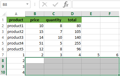
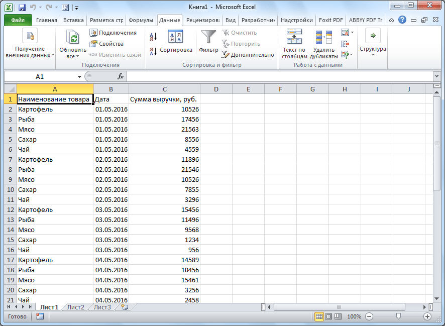
It`s the simplest and universal way. Let’s consider at once on an example. We have the table with the price of a certain product per a piece and with certain amount of products. The table cap is located horizontally, and the data is arranged vertically, respectively. The cost is calculated by the formula: price * quantity. For the sake of the clarity, the table header is highlighted in green color.
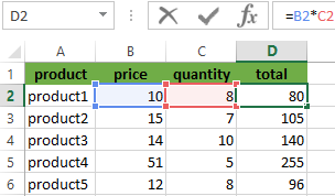
We need to arrange the table`s data horizontally relative to the vertical arrangement of its header.
To transpose the table, we will use the SPECIAL INSERT command. We proceed in these steps:
- We select the entire table and copy it (CTRL + C).
- We put the cursor anywhere in the Excel worksheet and right-click the menu.
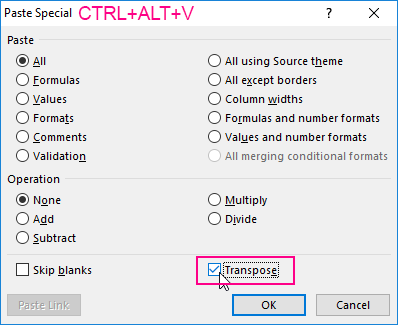
- We click on the command Paste Special (CTRL+ALT+V).
- In the window that appears we put the tick near the TRANSPOSE. The rest we left as is and click OK.
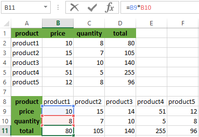
As a result we obtained the same table, but with different arrangement of the rows and the columns. Moreover, we note that cells with the same content are highlighted in green. The value formula was also copied and counted the product of price and quantity, but already with taking into account other cells. Now the table header is located vertically (what is clearly visible due to the green color of the header), and the data are respectively located horizontally.
Similarly, only values can be transposed, without the names of rows and the columns. To do this, you need to select only the array with the values and to do the same with the «Paste Special» command.
The method 2: the TRANSPOSE function in Excel
With the advent of the SPECIAL INSERT, the transposing of the table with using the TRANSPOSE command is almost not used because of the complexity and longer time for the operation. But the TRANSPOSE function is still present in Excel, so we will learn how to use it.
We operate on the stages again:
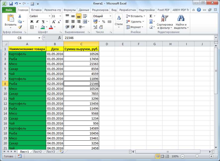
- We select correctly to the range for transposing. In this example of the source table there are 4 columns and 6 rows. Accordingly, we must select the range of the cells in what there will be 6 columns and 4 rows. As it shown on the picture:
- We fill immediately to the active cell so that you do not remove the selected area and enter the following formula: =TRANSPOSE.
- To press CTRL + SHIFT + ENTER. Attention! The function TRANSPOSE() works only in an array. Therefore, after entering it, you must necessarily press the combination of the hotkeys CTRL + SHIFT + ENTER to execute the function in the array, and not just ENTER.

Note that the formula was not copied. When you click on the each cell, you will see that this table has been transposed. In addition, all the original formatting has been lost and you have to align and backlight it again. Also worth paying attention to the fact that the transposed table is tied to the original one. The modified values of the source table are automatically updated in the transposed one.
The method 3: the PivotTable
Those who work closely with Excel know that the PivotTable is multifunctional. And possibility of transpose – is one of its functions. Although it will be look a little bit different than in the previous examples.
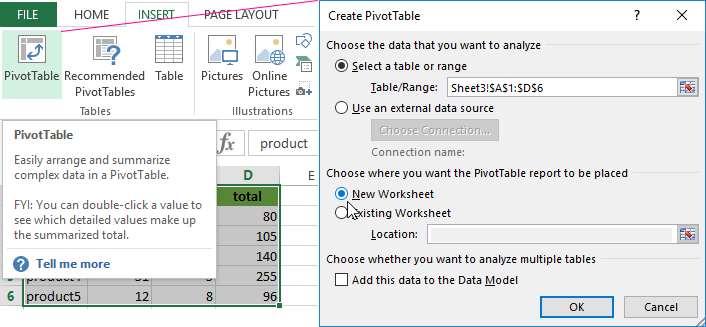
- We will create to the PivotTable. To do this, you need to select the original table and open the INSERT — PivotTable item.
- The place where the summary table will be created, we select the new sheet.
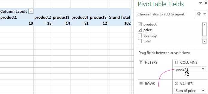
- In the resulting layout of the summary tables, we can select the necessary items and move them to the required fields. We will transfer «product» in the NAMES of COLUMNS, and «the price per piece» in VALUES.
- We obtained the PivotTable for the required field, and the team automatically calculated the grand total.
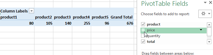
- You can remove the tick from the PRICE and tick off it next to the TOTAL PRICE. And then we get the PivotTable for the value of goods, as well as the grand total again.
Download example transpose data in Excel.
This is a rather peculiar method of partial transposition, which allows you to replace the columns in the rows (on the contrary — it does not work) and additionally learn to the total amount of the given field.
Как перенести таблицу в Экселе?
Также статьи о работе с таблицами в Экселе:
Не всегда созданные в Excel таблицы удачно размещены на листе, так как не всегда известен их окончательный размер. Как известно, вся область листа Excel может быть разбита на страницы для вывода на печать, и далее мы рассмотрим, как перенести таблицу в Экселе для более удобного расположения на странице.
Таблицы могут быть составлены как вводом данных вручную, так с помощью расчетов, т.е. в каждой ячейке таблицы будет находится формула. Перенести таблицу в Excel можно как с сохранением всех формул, так и перенести только результаты вычислений.
Самый простой способ перенести таблицу в Экселе, это выделить ее и перетащить мышкой в необходимый участок листа. После выделения таблицы необходимо подвести курсор к краю таблицы и после появления черного крестика со стрелками зажать левую кнопку мыши и перетащить таблицу.

При перетаскивании таблицы таким способом в ней сохраняются все формулы и автоматически меняются в них адреса ячеек, благодаря чему результаты расчетов не меняются. При желании можно в Экселе перенести таблицу на другой лист, для чего потребуется при перетаскивании мышкой зажать клавишу «Alt».
Также перенос таблиц в Excel можно организовать используя комбинацию клавиш «Ctrl + X» для вырезания с текущего расположения на листе, и комбинацию «Ctrl + V» для установки таблицы на новое место. Вместо комбинации клавиш можно воспользоваться соответствующими пунктами меню на вкладке «Главная».

Перемещение и копирование ячеек, строк и столбцов
Примечание: Мы стараемся как можно оперативнее обеспечивать вас актуальными справочными материалами на вашем языке. Эта страница переведена автоматически, поэтому ее текст может содержать неточности и грамматические ошибки. Для нас важно, чтобы эта статья была вам полезна. Просим вас уделить пару секунд и сообщить, помогла ли она вам, с помощью кнопок внизу страницы. Для удобства также приводим ссылку на оригинал (на английском языке).
При перемещении или копировании строк и столбцов приложение Excel перемещает или копирует все содержащиеся в них данные, в том числе формулы и значения их результатов, примечания, форматы ячеек и скрытые ячейки.
Если ячейка имеет формулу, ссылка на ячейку не изменяется. Таким образом, содержимое перемещенной или скопированной ячейки и ячеек, указывающих на них, может отобразить #REF! значение ошибки #ЗНАЧ!. В этом случае вам придется настроить ссылки вручную. Дополнительные сведения можно найти в разделе Обнаружение ошибок в формулах
Вы можете использовать команду Вырезать или Копировать для перемещения или копирования выделенных ячеек, строк и столбцов, но вы также можете перемещать или копировать их с помощью мыши.
Чтобы переместить или скопировать ячейки, сделайте следующее:
Выделите ячейку, строку или столбец , которые нужно переместить или скопировать.
Выполните одно из следующих действий.
Чтобы переместить строки или столбцы, на вкладке Главная в группе Буфер обмена нажмите кнопку Вырезать  .
.

Сочетание клавиш: CTRL+X.
Чтобы скопировать строки или столбцы, на вкладке Главная в группе Буфер обмена нажмите кнопку Копировать  .
.
Сочетание клавиш: CTRL+C.
Щелкните правой кнопкой мыши строку или столбец снизу или справа от того места, куда необходимо переместить или скопировать выделенный элемент, а затем выполните одно из указанных ниже действий.
Чтобы переместить строки или столбцы, выберите в контекстном меню команду Вставить вырезанные ячейки.
Чтобы скопировать строки или столбцы, выберите в контекстном меню команду Вставить скопированные ячейки.
Примечание: Если вместо выбора команды в контекстном меню нажать кнопку Вставить  на вкладке Главная в группе Буфер обмена (или нажать клавиши CTRL+V), содержимое конечных ячеек будет заменено.
Перемещение и копирование строк и столбцов с помощью мыши
Выделите строки или столбцы, которые вы хотите переместить или скопировать.
Выполните одно из указанных ниже действий.
Чтобы переместить строки или столбцы, наведите указатель мыши на границу выделения. Когда указатель примет вид указателя перемещения  , перетащите строки или столбцы в нужное место.
Чтобы скопировать строки или столбцы, нажмите клавишу CTRL и, удерживая ее, наведите указатель мыши на границу выделения. Когда указатель мыши примет вид указателя копирования  , перетащите строки или столбцы в нужное место.
Важно: При перетаскивании удерживайте клавишу CTRL нажатой. Если отпустить клавишу CTRL раньше кнопки мыши, строки или столбцы будут перемещены, а не скопированы.
Если вставка скопированных или вырезанных столбцов или строк выполняется с помощью мыши, содержимое конечных ячеек заменяется. Чтобы вставить скопированные или вырезанные строки или столбцы без замены содержимого ячеек, щелкните правой кнопкой мыши строку или столбец снизу или справа от того места, куда требуется переместить или скопировать выделенный элемент, а затем в контекстном меню выберите команду Вставить вырезанные ячейки или Вставить скопированные ячейки.
Примечание: С помощью мыши невозможно переместить или скопировать несмежные строки или столбцы.
Перемещение и копирование ячеек
Выделите ячейки или диапазон ячейки, которые вы хотите переместить или скопировать.
Наведите указатель мыши на границу выбранной ячейки или диапазона.
Когда указатель превратится в  , выполните одно из следующих действий:
Как в excel переместить таблицу
Всем, кто работает с Excel, периодически приходится переносить данные из одной таблицы в другую, а зачастую и просто копировать массивы в разные файлы. При этом необходимо сохранять исходные форматы ячеек, формулы, что в них находятся, и прочие переменные, которые могут потеряться при неправильном переносе.
Давайте разберёмся с тем, как переносить таблицу удобнее всего и рассмотрим несколько способов. Вам останется лишь выбрать тот, что наилучшим образом подходит к конкретной задачи, благо Microsoft побеспокоилась об удобстве своих пользователей в любой ситуации.
Копирование таблицы с сохранением структуры
Если у вас есть одна или несколько таблиц, форматирование которых необходимо сохранять при переносе, то обычный метод Ctrl+C – Ctrl+V не даст нужного результата.

В результате мы получим сжатые или растянутые ячейки, которые придётся вновь выравнивать по длине, чтобы они не перекрывали информацию.

Расширять вручную таблицы размером в 20-30 ячеек, тем более, когда у вас их несколько, не самая увлекательная задача. Однако существует несколько способов значительно упростить и оптимизировать весь процесс переноса при помощи инструментов, уже заложенных в программу.
Способ 1: Специальная вставка
Этот способ подойдёт в том случае, если из форматирования вам достаточно сохранить ширину столбцов и подтягивать дополнительные данные или формулы из другого файла/листа нет нужды.
- Выделите исходные таблицы и проведите обычный перенос комбинацией клавиш Ctrl+C – Ctrl+V.
- Как мы помним из предыдущего примера, ячейки получаются стандартного размера. Чтобы исправить это, выделите скопированный массив данных и кликните правой кнопкой по нему. В контекстном меню выберите пункт «Специальная вставка».

Нам потребуется «Ширины столбцов», поэтому выбираем соответствующий пункт и принимаем изменения.

В результате у вас получится таблица идентичная той, что была в первом файле. Это удобно в том случае, если у вас десятки столбцов и выравнивать каждый, стандартными инструментами, нет времени/желания. Однако в этом методе есть недостаток — вам все равно придётся потратить немного времени, ведь изначально скопированная таблица не отвечает нашим запросам. Если это для вас неприемлемо, существует другой способ, при котором форматирование сохранится сразу при переносе.
Способ 2: Выделение столбцов перед копированием
В этом случае вы сразу получите нужный формат, достаточно выделить столбцы или строки, в зависимости от ситуации, вместе с заголовками. Таким образом, изначальная длина и ширина сохранятся в буфере обмена и на выходе вы получите нужный формат ячеек. Чтобы добиться такого результата, необходимо:
- Выделить столбцы или строки с исходными данными.

- Просто скопировать и вставить, получившаяся таблица сохранит изначальный вид.

В каждом отдельном случае рациональней использовать свой способ. Однако он будет оптимален для небольших таблиц, где выделение области копирования не займёт у вас более двух минут. Соответственно, его удобно применять в большинстве случаев, так как в специальной вставке, рассмотренной выше, невозможно сохранить высоту строк. Если вам необходимо выровнять строки заранее – это лучший выбор. Но зачастую помимо самой таблицы необходимо перенести и формулы, что в ней хранятся. В этом случае подойдёт следующий метод.
Способ 3: Вставка формул с сохранением формата
Специальную вставку можно использовать, в том числе, и для переноса значений формул с сохранением форматов ячеек. Это наиболее простой и при этом быстрый способ произвести подобную операцию. Может быть удобно при формировании таблиц на распечатку или отчётностей, где лишний вес файла влияет на скорость его загрузки и обработки.
Чтобы выполнить операцию, сделайте следующее:
- Выделите и скопируйте исходник.
- В контекстном меню вставки просто выберите «Значения» и подтвердите действие.

Вместо третьего действия можно использовать формат по образцу. Подойдёт, если копирование происходит в пределах одного файла, но на разные листы. В простонародье этот инструмент ещё именуют «метёлочкой».
Перенос таблицы из одного файла в другой не должен занять у вас более пары минут, какое бы количество данных не находилось в исходнике. Достаточно выбрать один из описанных выше способов в зависимости от задачи, которая перед вами стоит. Умелое комбинирование методов транспортировки таблиц позволит сохранить много нервов и времени, особенно при составлении квартальных сводок и прочей отчётности. Однако не забывайте, что сбои могут проходить в любой программе, поэтому перепроверяйте данные, прежде чем отправить их на утверждение.
Вставка таблицы из программы Word в Microsoft Excel

Чаще приходится переносить таблицу из программы Microsoft Excel в приложение Word, чем наоборот, но все-таки случаи обратного переноса тоже не столь редки. Например, иногда требуется перенести таблицу в Excel, сделанную в Ворде, для того чтобы, воспользовавшись функционалом табличного редактора, рассчитать данные. Давайте выясним, какие способы переноса таблиц в данном направлении существуют.
Обычное копирование
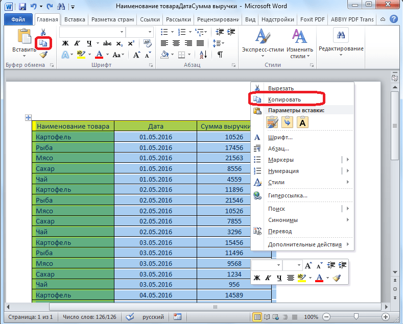
Самый простой способ переноса таблицы выполняется методом обычного копирования. Для этого, выделяем таблицу в программе Word, кликаем правой кнопкой мыши по странице, и в появившемся контекстном меню выбираем пункт «Копировать». Можно, вместо этого, нажать на кнопку «Копировать», которая размещена вверху на ленте. Ещё один вариант предполагает, после выделения таблицы, нажатие на клавиатуре клавиш Ctrl+C.
Таким образом, мы скопировали таблицу. Теперь нам нужно вставить её на лист Excel. Запускаем программу Microsoft Excel. Кликаем по ячейке в том месте листа, где хотим разместить таблицу. Нужно заметить, что эта ячейка станет крайней левой верхней ячейкой вставляемой таблицы. Именно из этого нужно исходить, планируя размещения таблицы.
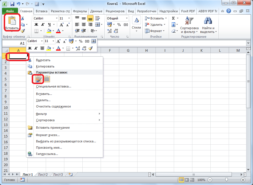
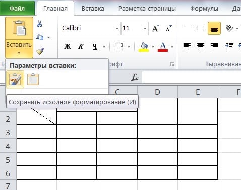
Кликаем правой кнопкой мыши по листу, и в контекстном меню в параметрах вставки выбираем значение «Сохранить исходное форматирование». Также, можно вставить таблицу, нажав на кнопку «Вставить», расположенную на левом краю ленты. Или же, существует вариант набрать на клавиатуре комбинацию клавиш Ctrl+V.
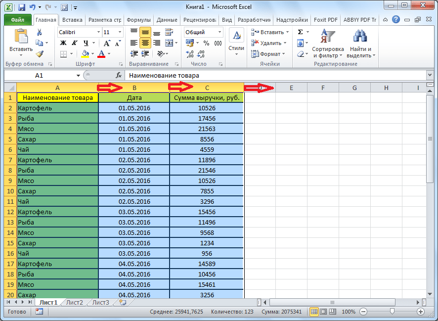
После этого, таблица будет вставлена на лист Microsoft Excel. Ячейки листа могут не совпадать с ячейками вставленной таблицы. Поэтому, чтобы таблица выглядела презентабельно, их следует растянуть.
Импорт таблицы
Также, существует более сложный способ переноса таблицы из Word в Excel, путем импорта данных.
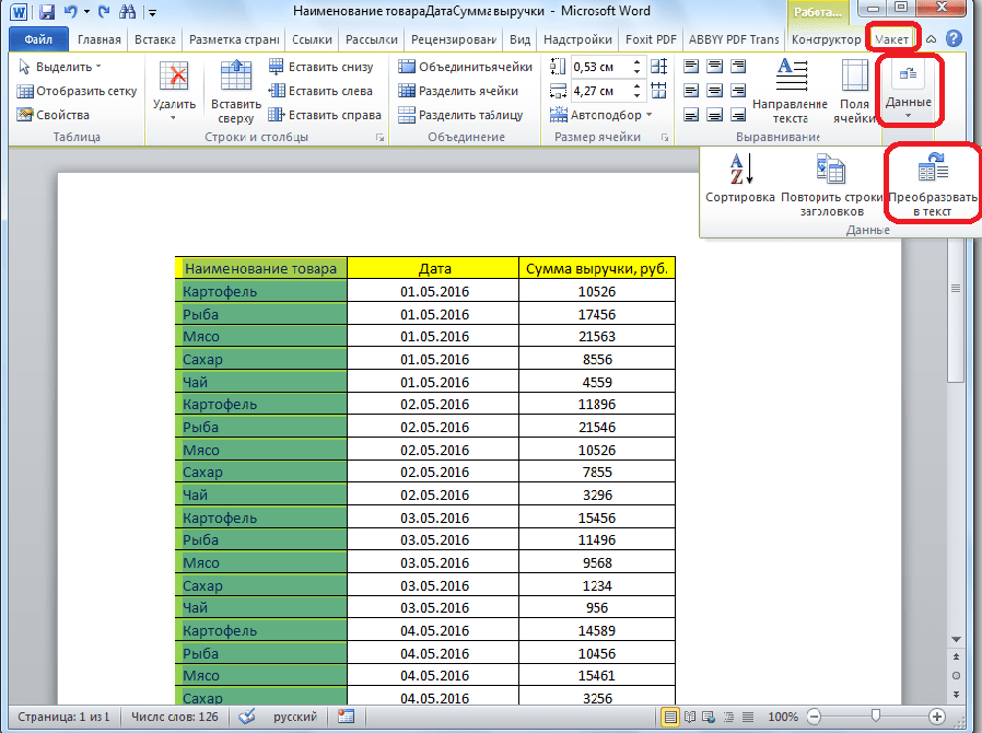
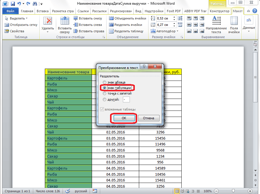
Открываем таблицу в программе Word. Выделяем её. Далее, переходим во вкладку «Макет», и в группе инструментов «Данные» на ленте жмем на кнопку «Преобразовать в текст».
Открывается окно параметров преобразования. В параметре «Разделитель» переключатель должен быть выставлен на позицию «Знак табуляции». Если это не так, переводим переключатель в данную позицию, и жмем на кнопку «OK».
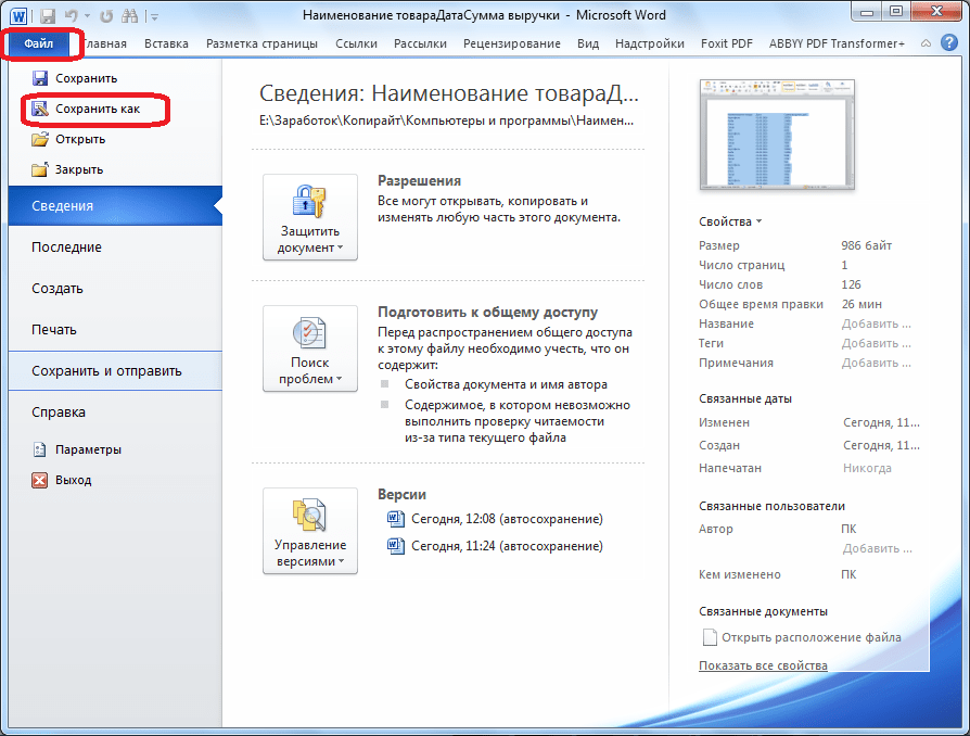
Переходим во вкладку «Файл». Выбираем пункт «Сохранить как…».
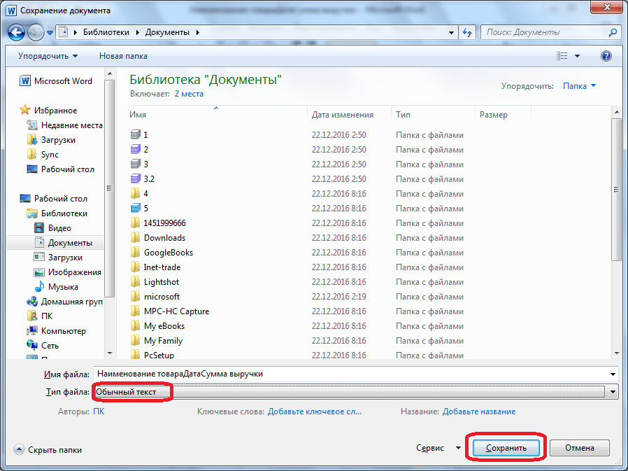
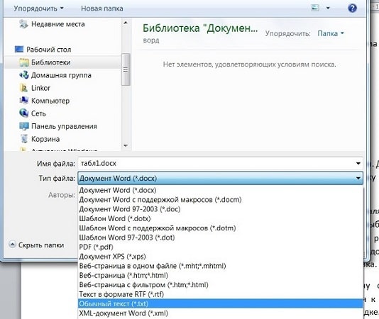
В открывшемся окне сохранения документа, указываем желаемое место расположения файла, который собираемся сохранить, а также присваиваем ему название, если название по умолчанию не удовлетворяет. Хотя, учитывая, что сохраненный файл будет являться лишь промежуточным для переноса таблицы из Word в Excel, особого смысла менять наименование нет. Главное, что нужно сделать – это в поле «Тип файла» установить параметр «Обычный текст». Жмем на кнопку «Сохранить».
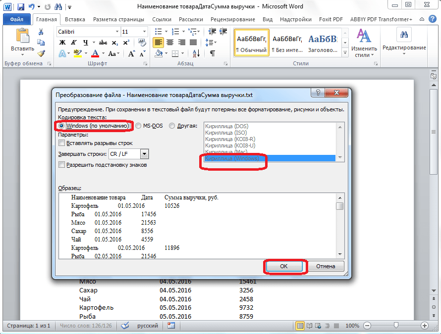
Открывается окно преобразования файла. Тут делать никаких изменений не нужно, а только следует запомнить кодировку, в которой вы сохраняете текст. Жмем на кнопку «OK».
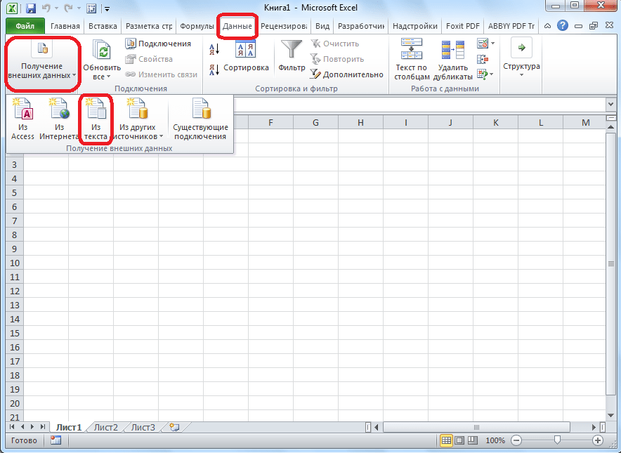
После этого, запускаем программу Microsoft Excel. Переходим во вкладку «Данные». В блоке настроек «Получить внешние данные» на ленте жмем на кнопку «Из текста».
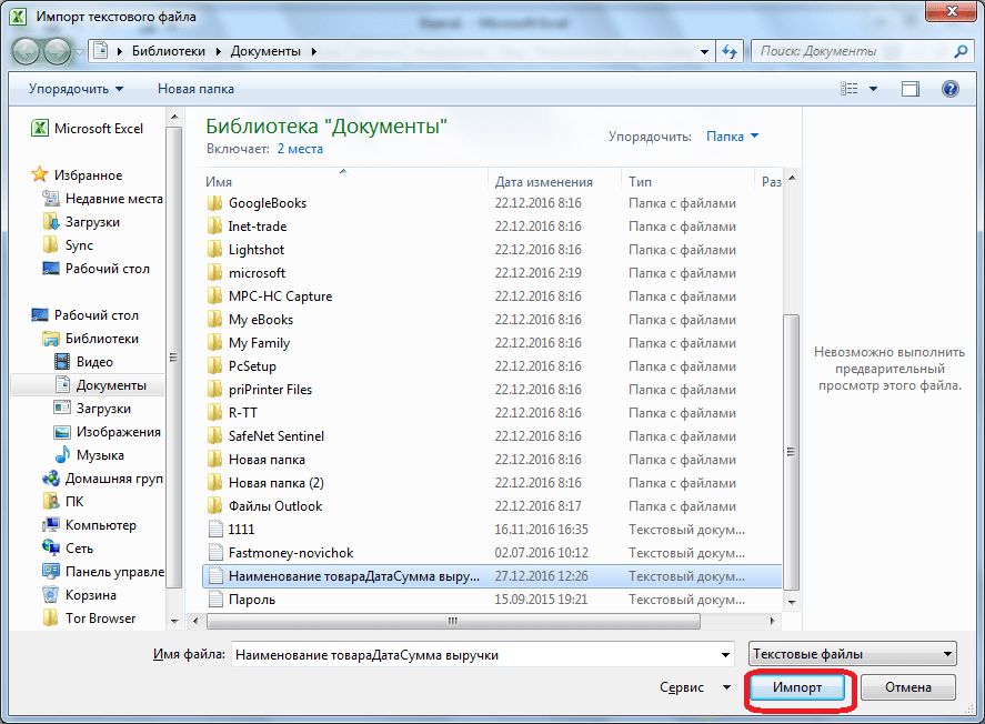
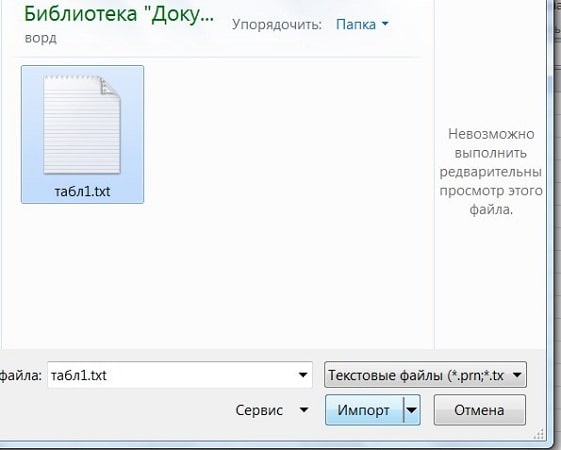
Открывается окно импорта текстового файла. Ищем тот файл, который сохранили ранее в Ворде, выделяем его, и жмем на кнопку «Импорт».
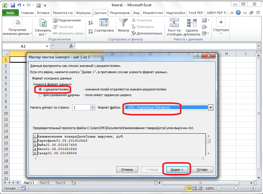
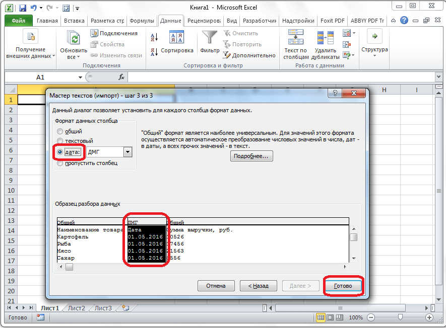
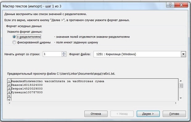
После этого, открывается окно Мастера текстов. В настройках формата данных указываем параметр «С разделителями». Устанавливаем кодировку, согласно той, в которой вы сохраняли текстовый документ в Ворде. В большинстве случаев это будет «1251: Кириллица (Windows)». Жмем на кнопку «Далее».
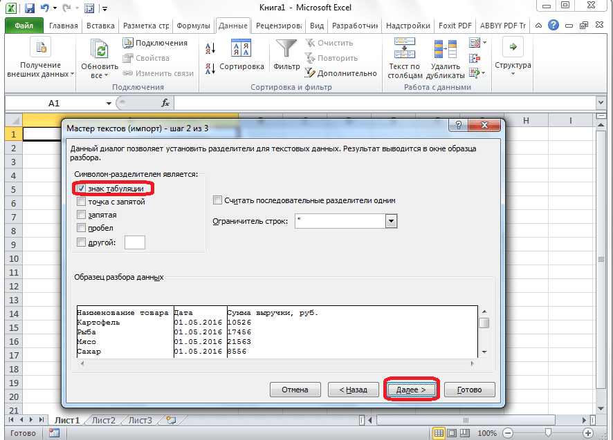
В следующем окне в настройке «Символом-разделителем является» устанавливаем переключатель в позицию «Знак табуляции», если он не установлен по умолчанию. Жмем на кнопку «Далее».
В последнем окне Мастера текста можно отформатировать данные в столбцах, с учетом их содержимого. Выделяем конкретный столбец в Образце разбора данных, а в настройках формата данных столбца выбираем один из четырёх вариантов:
Подобную операцию делаем для каждого столбца в отдельности. По окончанию форматирования, жмем на кнопку «Готово».
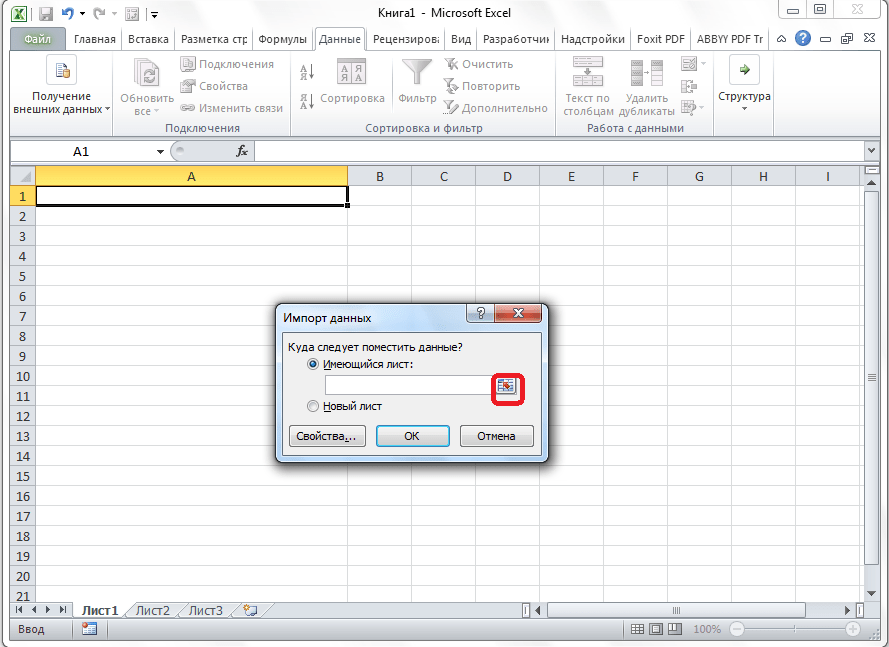
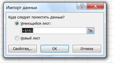
После этого, открывается окно импорта данных. В поле вручную указываем адрес ячейки, которая будет являться крайней верхней левой ячейкой вставленной таблицы. Если вы затрудняетесь это сделать вручную, то жмем на кнопку справа от поля.
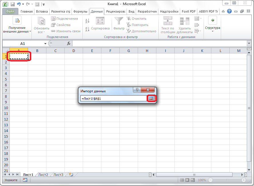
В открывшемся окне, просто выделяем нужную ячейку. Затем, кликаем по кнопке справа от введенных в поле данных.
Возвратившись в окно импорта данных, жмем на кнопку «OK».
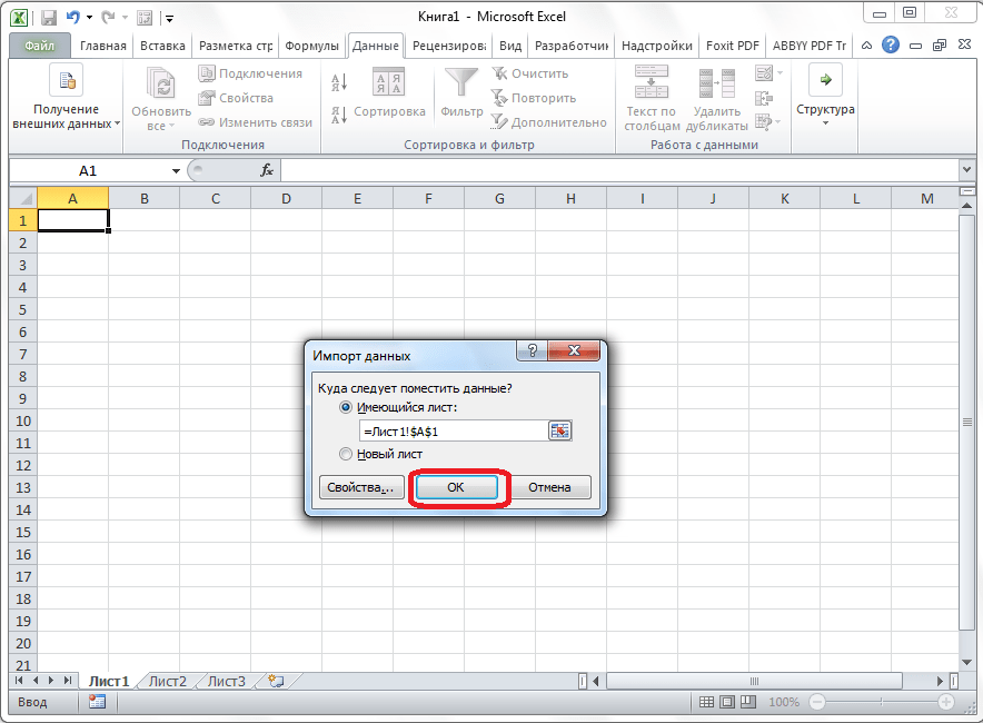
Как видим, таблица вставлена.
Далее, при желании, можно установить для неё видимые границы, а также отформатировать стандартными способами Microsoft Excel.
Выше были представлены два способа переноса таблицы из Word в Excel. Первый способ намного проще второго, и на всю процедуру уходит гораздо меньше времени. В то же время, второй способ гарантирует отсутствие лишних символов, или смещения ячеек, что вполне возможно при переносе первым способом. Так что, определяться с вариантом переноса, нужно отталкиваясь от сложности таблицы, и её предназначения.
Отблагодарите автора, поделитесь статьей в социальных сетях.
Как перенести таблицу из Word в Excel
Ситуация, когда из ворда в эксель нужно переместить табличку с данными, встречается не так часто. Например, это может пригодиться, чтобы воспользоваться специальными формулами и быстро произвести какие-либо подсчеты. В статье рассмотрим пошаговую инструкцию, как перенести таблицу из Word в Excel.

Простое копирование
Первым и самым простым способом для переноса таблицы из ворда в эксель является ее простое копирование из исходного документа с последующей вставкой в другой. Поэтапно это делается следующим образом:
-
Сначала нужно выделить всю таблицу, нажав на значок в виде двух пересекающихся двухсторонних стрелок в верхнем левом углу.


После выполнения данной последовательности нужная таблица появится на листе эксель. Однако иногда информация, помещенная в ячейки, не отображается полностью. Тогда следует вручную растянуть столбцы и строки.
Импортирование данных из Word в Excel
Существует и другой вариант, который считается более сложным. Он позволяет не копировать и вставлять вручную, а импортировать данные из таблица с сохранением параметров. Пользователь, который хочет воспользоваться данным методом, должен четко следовать алгоритму действий, описанных ниже:
- Открыть исходную таблицу в программе Word и выделить ее, нажав на уже упомянутый в прошлом разделе значок со стрелками, появившийся в левом углу.
- Перейти в «Макет» в панели инструментов (в разделе «Работа с таблицами»).
- В самом правом разделе панели инструментов под названием «Данные» имеется функция «Преобразовать в текст».

В появившемся окне параметров нужно выбрать знак табуляции в качестве «Разделителя». Подтвердить выбор нажатием «Ок».

Перейти во вкладку «Файл» и нажать пункт «Сохранить как». Далее указываем место, где будет располагаться документ, даем ему наименование. Главное, что важно сделать, — это изменить тип файла. Он должен быть обычным текстом (.txt).
Нажать «Сохранить». В открывшемся окне преобразования ничего менять не понадобится. Нужно только запомнить кодировку, например Windows (по умолчанию).

-
Перейти во вкладку «Данные», последовательно нажать «Получение внешних данных» — «Из текста».

Далее перед пользователем появится окно, именуемое «Мастер текстов». В нем в настройках следует отметить формат данных «с разделителем». Также нужно установить кодировку, в который был сохранен текстовый файл. После этого нажать «Далее».
В следующем окне в качестве символа-разделителя устанавливается знак табуляции и нажимается «Далее».

Финальным шагом является форматирование данных, при этом во внимание принимается содержимое ячеек. Так, по порядку нажимая каждый из столбцов, пользователь присваивает ему одно из значений (общий, текст, дата или пропустить). В конце нажимается «Готово».

На экране появится окно импорта, где указывается, на какой лист нужно поместить таблицу. Также в поле вводится адрес той ячейки, которая будет являться крайней левой верхней. Если вручную сделать это не получилось, следует кликнуть на кнопку, находящуюся рядом с полем для ввода данных. На сетке выделяем одним щелчком мыши нужную ячейку. После возврата в окно импорта данных нажимаем «Ок».
Перед пользователем появится таблица, которую в дальнейшем можно форматировать и редактировать встроенными инструментами.
Похожие статьи
Use Excel Tables to simplify your work! Learn how to create dynamic ranges, easy-to-read formulas using a table. In this tutorial, we’ll explain how to add new data to a range or how to manage Tables. Keep your formulas ready for auditing!
This guide provides useful tricks and examples.
- Fundamentals of Excel Tables
- Creating an Excel Table is Easy
- Add a name for a Table
- The Parts of a Table
- Navigating between Tables
- Table related Shortcuts
- Working with Tables
- Moving Excel Tables
- Swapping rows or columns in the table
- Keep Table headers always on the top
- Expand your Table easily
- Show Totals (Sum, Count, Min, Max) without using formulas
- Resize an Excel Table
- Table Formatting
- Change table formatting quickly
- Choose your Table style
- Tables and Data sources
- Quick Analysis works with Excel Tables
- Use a Table as a pivot table source
- Build dynamic charts using Tables
- Insert a new slicer into a table
- Convert Excel Tables to a normal range back
Fundamentals of Excel Tables
In this section, we’ll start with the basics.
Creating an Excel Table is Easy
How to create an Excel table?
- Select the range which contains data.
- Use the insert Table keyboard shortcut, Control + T
- If your table has headers, select the ‘My Table has headers’ checkbox.
- Click OK, and Excel will create a new table.
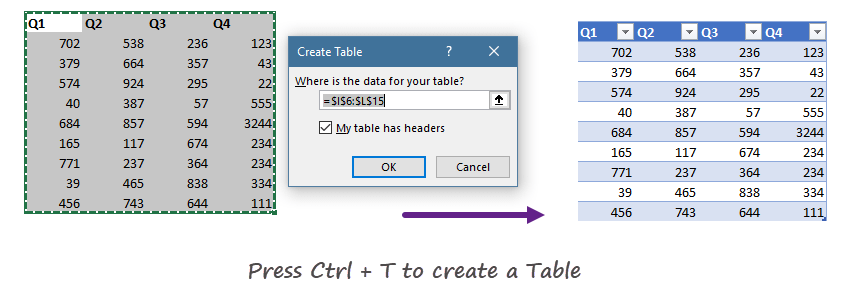
If you are in a hurry, Excel Tables is yours! On the right side of the picture, you’ll see banded rows.
Rename a Table
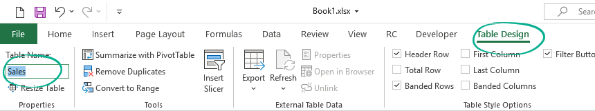
When you create a new Excel Table, Excel will assign a custom name, like Table1. You have to rename it and add a short, user-friendly name like ‘Sales.’
Important: Each table must have a unique name that contains letters, numbers, or the underscore character (for example, using spaces or special characters between words is not allowed.
To change the default name, select your table and locate the Table Design Tab. Jump to the Table Name > Properties section. Add a new name and press Enter.
The Parts of a Table
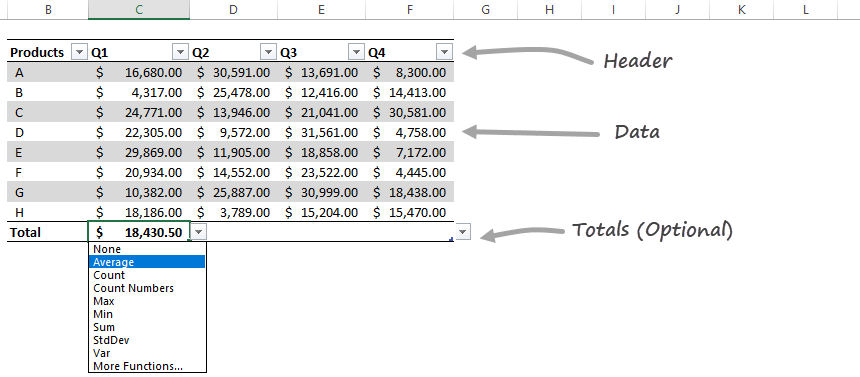
All Excel Tables have two required and one optional part.
The Column Header Row is the first row of the table. It contains identifiers, for example, ‘Product,’ ‘Order Date,’ and so on.
The body is the main data set.
Optional: you can switch an additional (Totals) row using the ‘Ctrl + Shift + T‘ shortcut.
Navigating between Tables
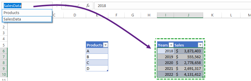
If you want to find your table quickly, locate the Name Box and use the drop-down menu in the top-left area of your workbook. Choose the table name, and what you want to activate. The range will be highlighted.
What if your table is located in a different tab? Excel will jump to the selected table.
If you have tabular data, you can easily convert it to an Excel Table.
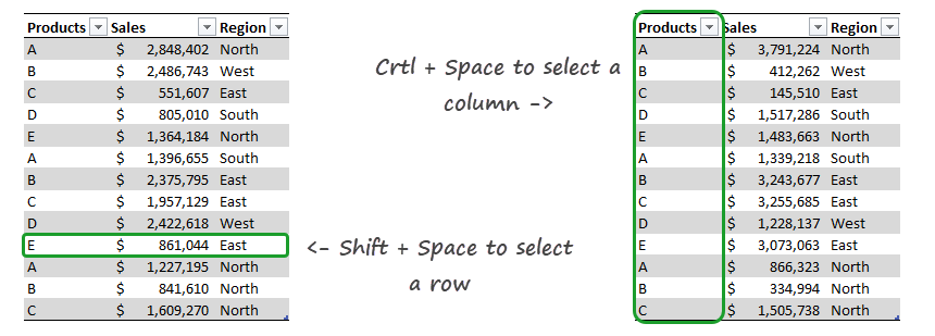
If you select a simple cell in the table, you can select the actual row using the ‘Shift + Space’ command. To select rows, use the ‘Control + Space’ keyboard shortcut.
Working with Tables
Moving Excel Tables
The easiest way to move a table to a new location is using a drag and drop method with a mouse.
In the example, we’ve just selected the original table then moved it to the K4:N13 range.
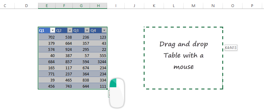
Tip: This is the fastest way to move tables to a new location. The method works only on the same sheet!
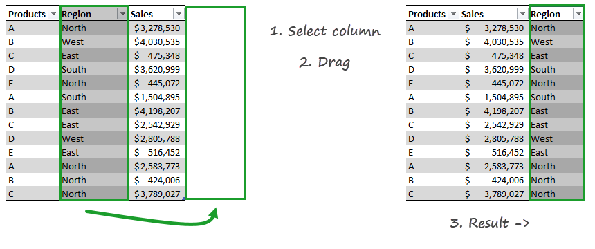
Swapping rows or columns in the table
It can frequently happen that you want to change the table structure or swap rows or columns. As first, select the table row or a table column. Make sure that the header row is selected. Drag the selected range and drop to a new area.
Excel will swap the given rows or columns. The method is safe because Excel will not overwrite the existing data.
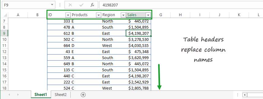
Excel Tables work simply. Are you working with large data sets? No problem! You can scroll down without any trouble. The table header will stay on the top. It’s not necessary to use the good old Freeze Top Rows function.
You can find it under the Freeze Panes group.
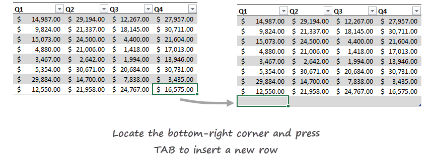
Expand your Table easily
In some cases, you need to insert rows or columns into an Excel Table. We’ll show you how to do that. The Excel Table is a dynamic range; it will resize even if you add or delete rows or columns.
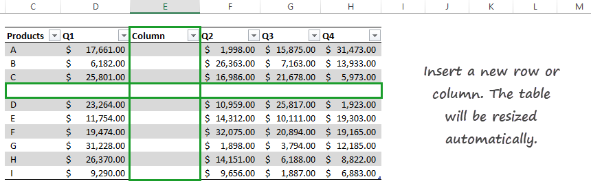
To add a new row, select the bottom-right cell in the range, in this example, cell F11. Press the Tab button; a new row appears, and the table structure remains.
It’s not necessary to select the range and add a new name for a range again.
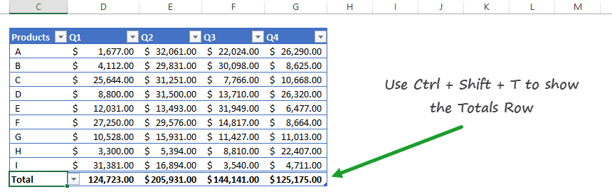
Show Totals (Sum, Count, Min, Max) without using formulas
With the help of tables, it’s easy to show dynamic Totals. Use your preferred formulas, like SUM, COUNT, AVERAGE, MIN, and MAX. Good to know that you don’t have to enter these formulas manually. Great!
You have a filtered Excel table on the left side and a regular table on the right side in the picture below. Use the ‘Control + Shift + T‘ shortcut to display the additional row under the table.
Resize an Excel Table
In the example below, you’ll learn how to change the table size using the ‘Resize Table’ command. This function is yours if you need to prepare a table for – for example – 500 rows.
To resize a table, select the new data range for your table. Click the OK button.
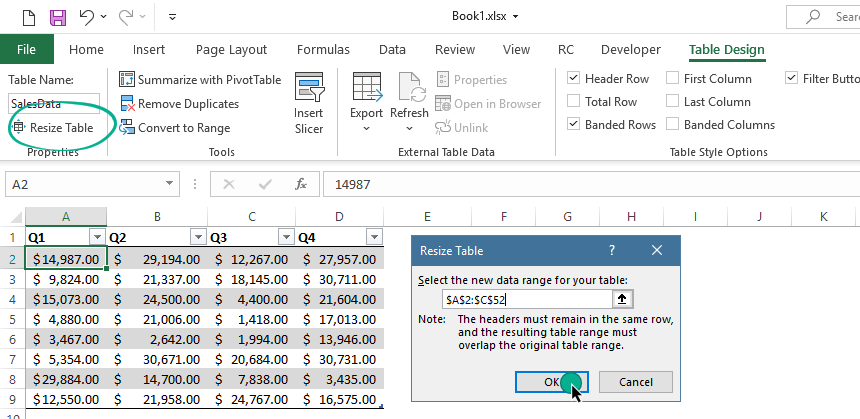
Note: The table headers must remain in the same row, and the resulting table range must overlap the original table range.
Or you can use the classic resize on the fly technic too. Select the small green triangle keeping the left mouse button pressed.
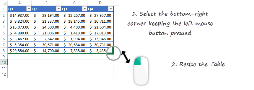
Table Formatting
Change table formatting quickly
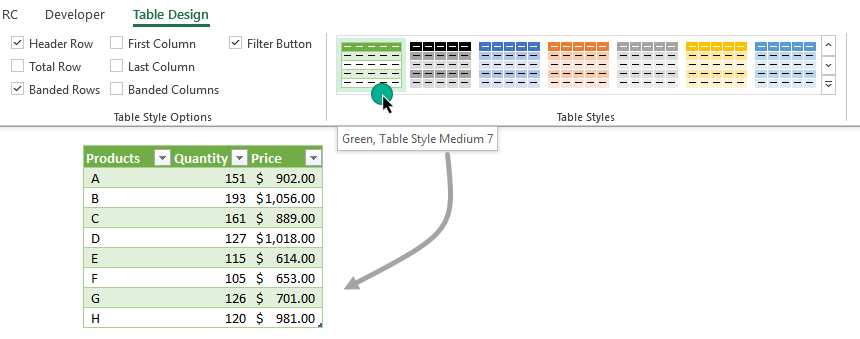
When you create a new table, it has a default formatting style. To override the displayed theme select a cell in the range. Choose the Table design tab on the ribbon and locate the Table Styles Group.
Click your preferred style, and the new theme will appear with a single click.
If you want to use the classic style without formatting, select the table and choose the default style by clicking on the top-left corner of the table style previews. The name of the first style is ‘None.’
Choose your Table style
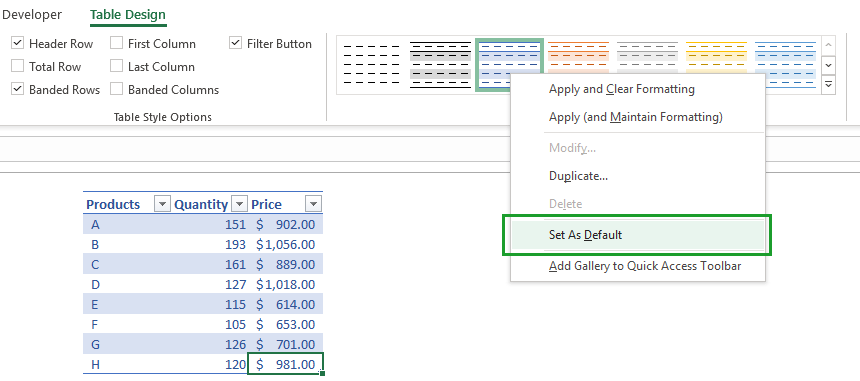
You can choose a default table style. What is the default style? Start Excel and create your first table. Excel assigns a built-in style to the table.
Select the style that you want to apply to all new tables in the future. Right-click on the Table preview and click on the ‘Set as default’ option.
Learn more on how to remove table formatting in Excel.
Tables and Data Sources
Quick Analysis works with Excel Tables
Everyone knows that the Quick Analysis Tool is a great function in Excel. Create your table first. After that, click Control + Q to create a floating row like in the picture below:
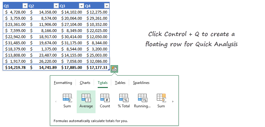
Apply various methods to analyze your data. Use conditional formatting, create chars, or calculate Totals, among others. If you need more power, use conditional formatting.
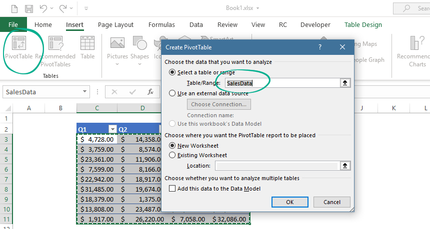
Use a Table as a pivot table source
Is it possible to use an Excel table as a pivot table source? Absolutely.
As we mentioned before, the Pivot table will track the changes in the table. If you add new data to the range, the pivot table will refresh automatically.
Go to the Insert tab. Insert a new pivot table.
A new window appears. Select the data that you want to analyze.
Finally, click OK.
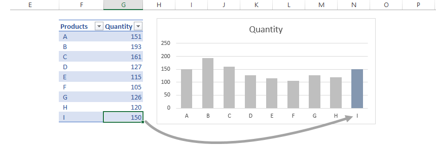
Build dynamic charts using Excel Tables
In our latest article, we’ve just talked about dynamic charts.
If you update your data frequently (adding rows or columns), tables are great for these purposes. Put your fresh data into the table, and the chart will refresh using the entered values.
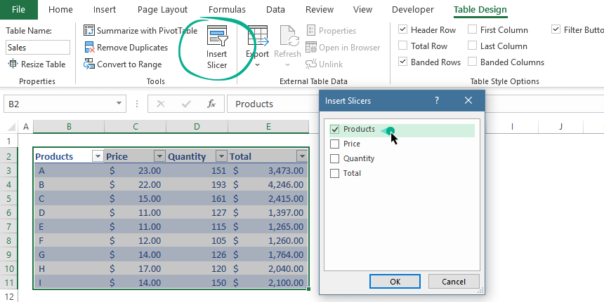
Insert a new slicer into a table
Good to know that all Excel Tables are slicer-ready? What does that mean in practice? Slicers are special filters. With its help, you can filter data quickly in various ways.
To add a new slicer:
- Select the table
- Locate the Table Design tab on the ribbon
- Locate the Tools group and Click the Insert Slicer button.
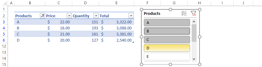
In the example below, now we have a slicer for Products:
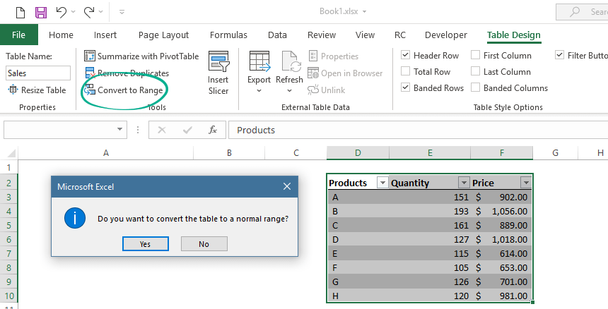
Convert Excel Tables to a normal range back
Tables are useful, but sometimes you need to work with normal ranges. To convert an Excel Table into a range back, do the following steps.
- Select the Table
- Remove the formatting style (choose the ‘None’ table style)
- Click on the Table Tools Tab
- Apply the ‘Convert to Range’ commands.
Note: Step 2 is necessary; otherwise, the formatting styles remain.
Conclusion
Excel Tables are versatile tools. With its help, you can speed up your daily tasks.
You May Also Like the Following Excel Tutorials:
- Creating an Excel Dashboard – The Ultimate Guide
- Structured references
Move a Pivot Table in the Same Worksheet or to a Different Worksheet in Microsoft Excel
by Avantix Learning Team | Updated March 15, 2021
Applies to: Microsoft® Excel® 2013, 2016, 2019 and 365 (Windows)
Moving a pivot table is not as simple as moving other objects in an Excel worksheet or workbook. You will typically need to use the Move PivotTable command in the Ribbon to move a pivot table to a different area on a worksheet or to a different sheet in the same workbook.
Note: Buttons and Ribbon tabs may display in a different way (with or without text) depending on your version of Excel, the size of your screen and your Control Panel settings. For Excel 365 users, Ribbon tabs may appear with different names. For example, the PivotTable Tools Analyze tab may appear as PivotTable Analyze.
Recommended article: How to Lock and Protect Excel Worksheets and Workbooks
Do you want to learn more about Excel? Check out our virtual classroom or live classroom Excel courses >
Moving a pivot table to a different location on the same worksheet
To move a pivot table on the same worksheet:
- Select a cell in the pivot table.
- Click the PivotTable Tools Analyze tab or PivotTable Analyze tab in the Ribbon.
- Click Move PivotTable in the Actions group. A dialog box appears.
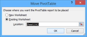
- Click in the Location box and then click the desired cell location on the current sheet for the top left cell of the pivot table. Excel will enter the name of the sheet and the cell reference.
- Click OK.
Below is the Move PivotTable dialog box in Excel:
Moving a pivot table to a different worksheet in the same workbook
To move a pivot table to a different sheet in the same workbook:
- Select a cell in the pivot table.
- Click the PivotTable Tools Analyze tab or PivotTable Analyze tab in the Ribbon.
- Click Move PivotTable in the Actions group. A dialog box appears.
- Click in the Location box.
- Select the sheet at the bottom that to which you want to move the pivot table.
- Click the desired cell location on the selected sheet for the top left cell of the pivot table. Excel will enter the name of the sheet and the cell reference.
- Click OK.
You can place multiple pivot tables on the same sheet using this method. It’s a good to leave some space if you have multiple pivot tables on the same worksheet.
Subscribe to get more articles like this one
Did you find this article helpful? If you would like to receive new articles, join our email list.
More resources
How to Convert Text to Numbers in Excel
How to Delete a Pivot Table in Microsoft Excel
How to Highlight Errors, Blanks and Duplicates in Excel Worksheets
Related courses
Microsoft Excel: Intermediate / Advanced
Microsoft Excel: Data Analysis with Functions, Dashboards and What-If Analysis Tools
Microsoft Excel: Introduction to Visual Basic for Applications (VBA)
VIEW MORE COURSES >
Our instructor-led courses are delivered in virtual classroom format or at our downtown Toronto location at 18 King Street East, Suite 1400, Toronto, Ontario, Canada (some in-person classroom courses may also be delivered at an alternate downtown Toronto location). Contact us at info@avantixlearning.ca if you’d like to arrange custom instructor-led virtual classroom or onsite training on a date that’s convenient for you.
Copyright 2023 Avantix® Learning
Microsoft, the Microsoft logo, Microsoft Office and related Microsoft applications and logos are registered trademarks of Microsoft Corporation in Canada, US and other countries. All other trademarks are the property of the registered owners.
Avantix Learning |18 King Street East, Suite 1400, Toronto, Ontario, Canada M5C 1C4 | Contact us at info@avantixlearning.ca