
When you move or copy rows and columns, by default Excel moves or copies all data that they contain, including formulas and their resulting values, comments, cell formats, and hidden cells.
When you copy cells that contain a formula, the relative cell references are not adjusted. Therefore, the contents of cells and of any cells that point to them might display the #REF! error value. If that happens, you can adjust the references manually. For more information, see Detect errors in formulas.
You can use the Cut command or Copy command to move or copy selected cells, rows, and columns, but you can also move or copy them by using the mouse.
By default, Excel displays the Paste Options button. If you need to redisplay it, go to Advanced in Excel Options. For more information, see Advanced options.
-
Select the cell, row, or column that you want to move or copy.
-
Do one of the following:
-
To move rows or columns, on the Home tab, in the Clipboard group, click Cut
 or press CTRL+X.
 -
To copy rows or columns, on the Home tab, in the Clipboard group, click Copy
or press CTRL+C.
-
-
Right-click a row or column below or to the right of where you want to move or copy your selection, and then do one of the following:
-
When you are moving rows or columns, click Insert Cut Cells.
-
When you are copying rows or columns, click Insert Copied Cells.
Tip: To move or copy a selection to a different worksheet or workbook, click another worksheet tab or switch to another workbook, and then select the upper-left cell of the paste area.
-
 or press CTRL+X.
 or press CTRL+C.
Note: Excel displays an animated moving border around cells that were cut or copied. To cancel a moving border, press Esc.
By default, drag-and-drop editing is turned on so that you can use the mouse to move and copy cells.
-
Select the row or column that you want to move or copy.
-
Do one of the following:
-
Cut and replace
Point to the border of the selection. When the pointer becomes a move pointer, drag the rows or columns to another location. Excel warns you if you are going to replace a column. Press Cancel to avoid replacing. -
Copy and replace Hold down CTRL while you point to the border of the selection. When the pointer becomes a copy pointer
, drag the rows or columns to another location. Excel doesn’t warn you if you are going to replace a column. Press CTRL+Z if you don’t want to replace a row or column. -
Cut and insert Hold down SHIFT while you point to the border of the selection. When the pointer becomes a move pointer
, drag the rows or columns to another location. -
Copy and insert Hold down SHIFT and CTRL while you point to the border of the selection. When the pointer becomes a move pointer
, drag the rows or columns to another location.
Note: Make sure that you hold down CTRL or SHIFT during the drag-and-drop operation. If you release CTRL or SHIFT before you release the mouse button, you will move the rows or columns instead of copying them.
-
 , drag the rows or columns to another location. Excel warns you if you are going to replace a column. Press Cancel to avoid replacing.
 , drag the rows or columns to another location. Excel doesn’t warn you if you are going to replace a column. Press CTRL+Z if you don’t want to replace a row or column.
Note: You cannot move or copy nonadjacent rows and columns by using the mouse.
If some cells, rows, or columns on the worksheet are not displayed, you have the option of copying all cells or only the visible cells. For example, you can choose to copy only the displayed summary data on an outlined worksheet.
-
Select the row or column that you want to move or copy.
-
On the Home tab, in the Editing group, click Find & Select, and then click Go To Special.
-
Under Select, click Visible cells only, and then click OK.
-
On the Home tab, in the Clipboard group, click Copy
or press Ctrl+C. . -
Select the upper-left cell of the paste area.
Tip: To move or copy a selection to a different worksheet or workbook, click another worksheet tab or switch to another workbook, and then select the upper-left cell of the paste area.
-
On the Home tab, in the Clipboard group, click Paste
or press Ctrl+V.If you click the arrow below Paste
, you can choose from several paste options to apply to your selection.
 or press Ctrl+V.
Excel pastes the copied data into consecutive rows or columns. If the paste area contains hidden rows or columns, you might have to unhide the paste area to see all of the copied cells.
When you copy or paste hidden or filtered data to another application or another instance of Excel, only visible cells are copied.
-
Select the row or column that you want to move or copy.
-
On the Home tab, in the Clipboard group, click Copy
or press Ctrl+C. -
Select the upper-left cell of the paste area.
-
On the Home tab, in the Clipboard group, click the arrow below Paste
, and then click Paste Special. -
Select the Skip blanks check box.
-
Double-click the cell that contains the data that you want to move or copy. You can also edit and select cell data in the formula bar.
-
Select the row or column that you want to move or copy.
-
On the Home tab, in the Clipboard group, do one of the following:
-
To move the selection, click Cut
or press Ctrl+X. -
To copy the selection, click Copy
or press Ctrl+C.
-
-
In the cell, click where you want to paste the characters, or double-click another cell to move or copy the data.
-
On the Home tab, in the Clipboard group, click Paste
or press Ctrl+V. -
Press ENTER.
Note: When you double-click a cell or press F2 to edit the active cell, the arrow keys work only within that cell. To use the arrow keys to move to another cell, first press Enter to complete your editing changes to the active cell.
When you paste copied data, you can do any of the following:
-
Paste only the cell formatting, such as font color or fill color (and not the contents of the cells).
-
Convert any formulas in the cell to the calculated values without overwriting the existing formatting.
-
Paste only the formulas (and not the calculated values).
Procedure
-
Select the row or column that you want to move or copy.
-
On the Home tab, in the Clipboard group, click Copy
or press Ctrl+C.
-
Select the upper-left cell of the paste area or the cell where you want to paste the value, cell format, or formula.
-
On the Home tab, in the Clipboard group, click the arrow below Paste
, and then do one of the following:-
To paste values only, click Values.
-
To paste cell formats only, click Formatting.
-
To paste formulas only, click Formulas.
-
When you paste copied data, the pasted data uses the column width settings of the target cells. To correct the column widths so that they match the source cells, follow these steps.
-
Select the row or column that you want to move or copy.
-
On the Home tab, in the Clipboard group, do one of the following:
-
To move cells, click Cut
or press Ctrl+X. -
To copy cells, click Copy
or press Ctrl+C.
-
-
Select the upper-left cell of the paste area.
Tip: To move or copy a selection to a different worksheet or workbook, click another worksheet tab or switch to another workbook, and then select the upper-left cell of the paste area.
-
On the Home tab, in the Clipboard group, click the arrow under Paste
, and then click Keep Source Column Widths.
You can use the Cut command or Copy command to move or copy selected cells, rows, and columns, but you can also move or copy them by using the mouse.
-
Select the cell, row, or column that you want to move or copy.
-
Do one of the following:
-
To move rows or columns, on the Home tab, in the Clipboard group, click Cut
or press CTRL+X. -
To copy rows or columns, on the Home tab, in the Clipboard group, click Copy
or press CTRL+C.
-
-
Right-click a row or column below or to the right of where you want to move or copy your selection, and then do one of the following:
-
When you are moving rows or columns, click Insert Cut Cells.
-
When you are copying rows or columns, click Insert Copied Cells.
Tip: To move or copy a selection to a different worksheet or workbook, click another worksheet tab or switch to another workbook, and then select the upper-left cell of the paste area.
-
Note: Excel displays an animated moving border around cells that were cut or copied. To cancel a moving border, press Esc.
-
Select the row or column that you want to move or copy.
-
Do one of the following:
-
Cut and insert
Point to the border of the selection. When the pointer becomes a hand pointer, drag the row or column to another location -
Cut and replace Hold down SHIFT while you point to the border of the selection. When the pointer becomes a move pointer
, drag the row or column to another location. Excel warns you if you are going to replace a row or column. Press Cancel to avoid replacing. -
Copy and insert Hold down CTRL while you point to the border of the selection. When the pointer becomes a move pointer
, drag the row or column to another location. -
Copy and replace Hold down SHIFT and CTRL while you point to the border of the selection. When the pointer becomes a move pointer
, drag the row or column to another location. Excel warns you if you are going to replace a row or column. Press Cancel to avoid replacing.
Note: Make sure that you hold down CTRL or SHIFT during the drag-and-drop operation. If you release CTRL or SHIFT before you release the mouse button, you will move the rows or columns instead of copying them.
-
 , drag the row or column to another location
Note: You cannot move or copy nonadjacent rows and columns by using the mouse.
-
Double-click the cell that contains the data that you want to move or copy. You can also edit and select cell data in the formula bar.
-
Select the row or column that you want to move or copy.
-
On the Home tab, in the Clipboard group, do one of the following:
-
To move the selection, click Cut
or press Ctrl+X. -
To copy the selection, click Copy
or press Ctrl+C.
-
-
In the cell, click where you want to paste the characters, or double-click another cell to move or copy the data.
-
On the Home tab, in the Clipboard group, click Paste
or press Ctrl+V. -
Press ENTER.
Note: When you double-click a cell or press F2 to edit the active cell, the arrow keys work only within that cell. To use the arrow keys to move to another cell, first press Enter to complete your editing changes to the active cell.
When you paste copied data, you can do any of the following:
-
Paste only the cell formatting, such as font color or fill color (and not the contents of the cells).
-
Convert any formulas in the cell to the calculated values without overwriting the existing formatting.
-
Paste only the formulas (and not the calculated values).
Procedure
-
Select the row or column that you want to move or copy.
-
On the Home tab, in the Clipboard group, click Copy
or press Ctrl+C.
-
Select the upper-left cell of the paste area or the cell where you want to paste the value, cell format, or formula.
-
On the Home tab, in the Clipboard group, click the arrow below Paste
, and then do one of the following:-
To paste values only, click Paste Values.
-
To paste cell formats only, click Paste Formatting.
-
To paste formulas only, click Paste Formulas.
-
You can move or copy selected cells, rows, and columns by using the mouse and Transpose.
-
Select the cells or range of cells that you want to move or copy.
-
Point to the border of the cell or range that you selected.
-
When the pointer becomes a
, do one of the following:
 , do one of the following:
|
To |
Do this |
|---|---|
|
Move cells |
Drag the cells to another location. |
|
Copy cells |
Hold down OPTION and drag the cells to another location. |
Note: When you drag or paste cells to a new location, if there is pre-existing data in that location, Excel will overwrite the original data.
-
Select the rows or columns that you want to move or copy.
-
Point to the border of the cell or range that you selected.
-
When the pointer becomes a
, do one of the following:
|
To |
Do this |
|---|---|
|
Move rows or columns |
Drag the rows or columns to another location. |
|
Copy rows or columns |
Hold down OPTION and drag the rows or columns to another location. |
|
Move or copy data between existing rows or columns |
Hold down SHIFT and drag your row or column between existing rows or columns. Excel makes space for the new row or column. |
-
Copy the rows or columns that you want to transpose.
-
Select the destination cell (the first cell of the row or column into which you want to paste your data) for the rows or columns that you are transposing.
-
On the Home tab, under Edit, click the arrow next to Paste, and then click Transpose.
Note: Columns and rows cannot overlap. For example, if you select values in Column C, and try to paste them into a row that overlaps Column C, Excel displays an error message. The destination area of a pasted column or row must be outside the original values.
See also
Insert or delete cells, rows, columns
Watch Video – The best way to Move Rows / Columns in Excel
Sometimes when working with data in Excel, you may have a need to move rows and columns in the dataset.
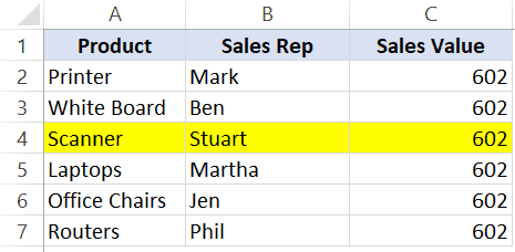
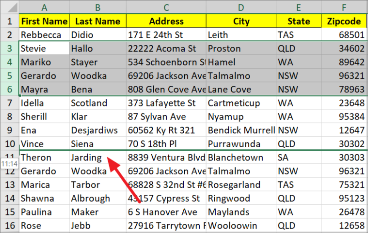
For example, in the below dataset, I want to quickly move the highlighted row to the top.
Now, are you thinking of copying this row, inserting the copied row where you want it, and then deleting it?
If yes – well that’s one way to do this.
But there is a lot faster way to move rows and columns in Excel.
In this tutorial, I will show you a fast way to move rows and columns in Excel – using an amazing shortcut.
Move Rows in Excel
Suppose I have the following dataset and I want to move the highlighted row to the second row (just below the headers):
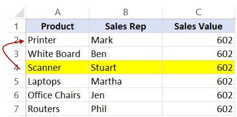
Here are the steps to do this:
- Select the row that you want to move.
- Hold the Shift Key from your keyboard.
- Move your cursor to the edge of the selection. It would display the move icon (a four directional arrow icon).
- Click on the edge (with left mouse button) while still holding the shift key.
- Move it to the row where you want this row to be shifted
- Leave the mouse button when you see a bold line right below the row where you want to move this row.
- Leave the Shift-key (remember to keep the Shift key pressed till the end)
Below is a video that shows how to move a row using this method.
Note that in this example, I have moved the selected cells only.
If you want to move the entire row, you can select the entire row and then follow the same steps.
Here are some important things to know about this method:
- You can move contiguous rows (or some cells from the contiguous rows). You can’t move non-contiguous rows using this method. For example, you can’t move row # 4 and 6 at the same time. However, you can move row #5 and 6 at the same time by selecting it.
- When you move some cells in a row/column using this method, it will not impact any other data in the worksheet. In the above example, any data outside (above/below or to the right/left of this table) remains unaffected.
Move Columns in Excel
The same technique can also be used to move columns in Excel.
Here are the steps:
- Select the column (or contiguous columns) that you want to move.
- Hold the Shift Key from your keyboard.
- Move your cursor to the edge of the selection. It would display the move icon (a four directional arrow icon).
- Click on the edge (with left mouse button) while still holding the shift key.
- Move it to the column where you want this row to be shifted
- Leave the mouse button when you see a bold line to the edge of the column where you want to move this column.
- Leave the Shift-key (remember to keep the Shift key pressed till the end).
You May Also Like the Following Excel Tutorials:
- Quickly select blank cells in Excel.
- Quickly select a far-off cell/range in Excel.
- Keyboard and Mouse tricks that will reinvent the way you Excel.
- Highlight every other row in Excel.
- Insert New Cells in Excel.
- Highlight Active Row/Column in a dataset.
- Delete rows based on cell value in Excel
- Insert New Columns in Excel
While working on a worksheet that has numerous rows of data, you may have to reorder the row and columns every now and then. Whether it’s a simple mistake or the data is not at the right spot or you simply need to rearrange the data, then you have to move rows or columns in Excel.
If you work with Excel tables a lot, it’s important to know how to move rows or columns in Excel. There are three ways to move rows or columns in Excel, including the drag method using the mouse, cut and paste, and rearrange rows using the Data Sort feature. In this tutorial, we will cover all three methods one by one.
Move a Row/Column by Dragging and Dropping in Excel
The drag and drop method is the easiest way to quickly move rows in a dataset. But dragging rows in Excel is a bit more complex than you realize. There are three ways you can drag-and-drop rows in Excel, including drag and replace, drag and copy, and drag and move.
Drag and Replace Row
The first method is a simple drag and drop but the moving row will replace the destination row.
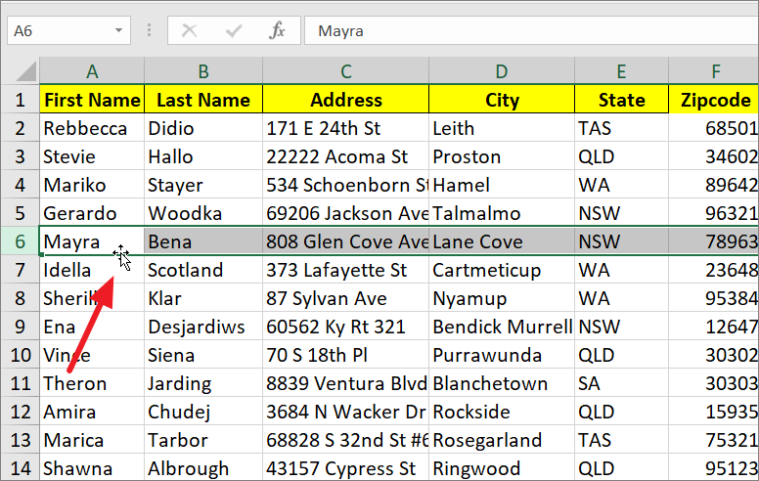
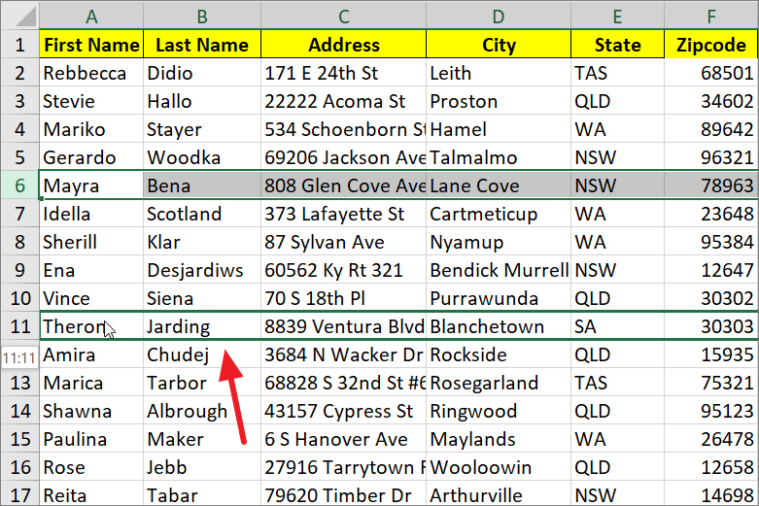
First, select the row (or contiguous rows) that you want to move. You can select an entire row by simply clicking the row number or clicking on any cell in the row and pressing Shift+Spacebar. Here, we’re selecting row 6.
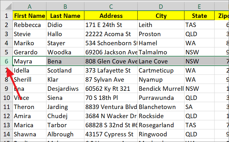
After selecting the row, move your cursor to the edge of the selection (either top or bottom). You should see your cursor change to a move pointer ![]() (cross with the arrows).
(cross with the arrows).
Now, hold down the left mouse click, and drag it (top or bottom) to the desired location where you want to move the row. While you’re dragging the row, it will highlight the current row in a green border. In the example, we’re dragging row 6 to row 11.
Then, release the left mouse button and you will see a pop-up asking “There’s already data here. Do you want to replace it?”. Click ‘OK’ to replace row 11 with the data of row 6.
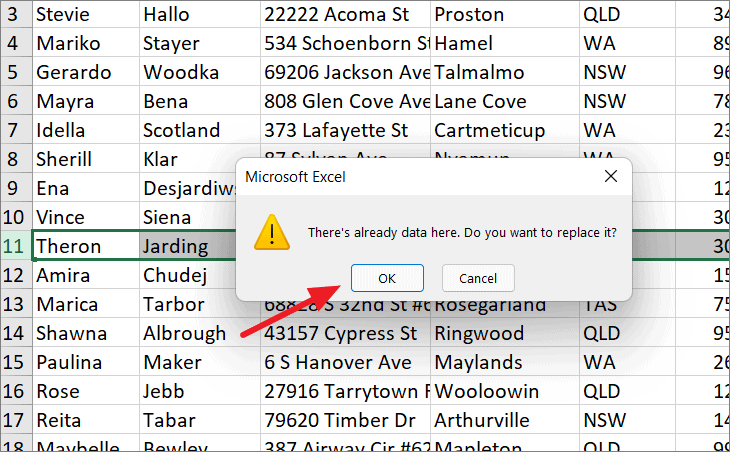
But, when you move your row to an empty row, Excel won’t show you this pop-up, it will simply move the data to the empty row.
In the below screenshot, you can see that row 11 is now replaced with row 6.
Drag and Move/Swap Row
You can quickly move or swap a row without overwriting the existing row by holding the Shift key when dragging the selected row(s).
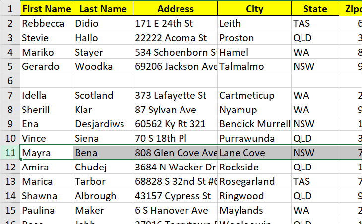
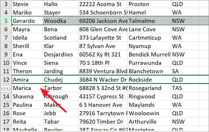
Select your row (or contiguous row) that you want to move the same you did in the above section. Here, we’re selecting row 5.
Next, press and hold the Shift key on the keyboard, move your cursor to the edge of the selection (either top or bottom). When your cursor turns to a move pointer ![]() (cross with the arrow), click on the edge (with left mouse button), and drag the row to the new location.
(cross with the arrow), click on the edge (with left mouse button), and drag the row to the new location.
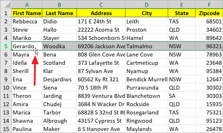
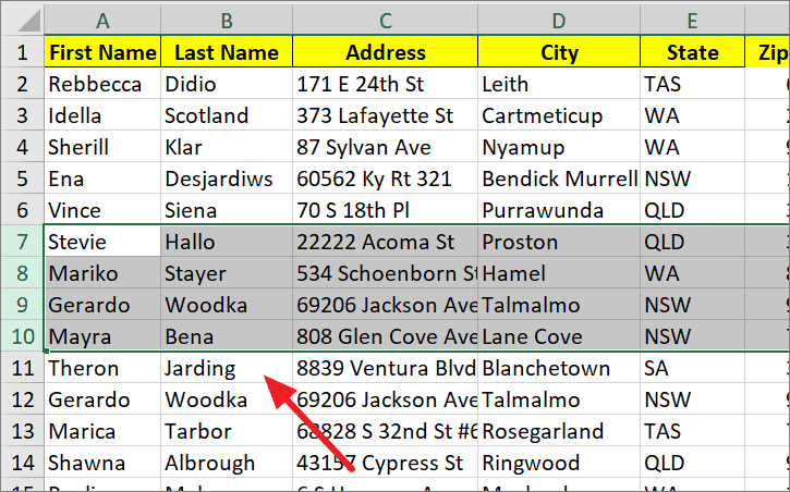
When you drag your cursor across the rows, you would see a bold green line at the edge of the row indicating where the new row will appear. Once you’ve found the right location for the row, release the mouse click and the Shift key. Here, we want to move row 5 to between rows 9 and 10.
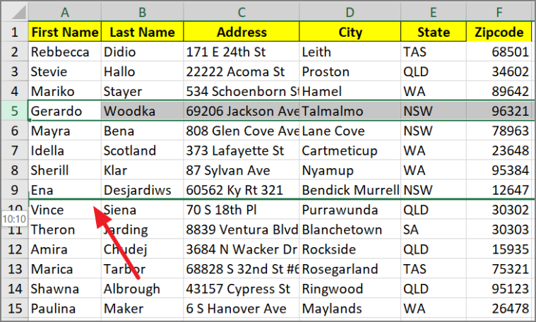
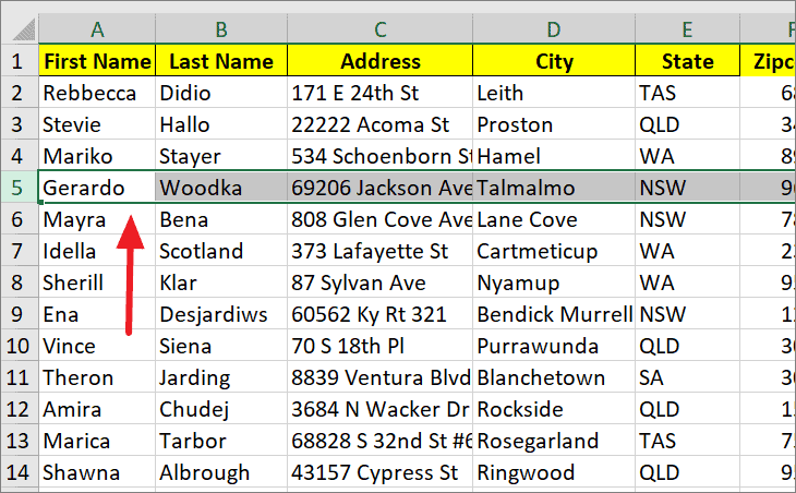
Once the mouse button is released, row 5 is moved to row 9, and the original row 9 automatically moves up.
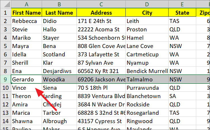
This method basically cuts the row and then inserts them to the new location (where you release the mouse button) without overwriting the existing row.
Drag and Copy Row
If you want to copy the row to the new location then simply press the Ctrl key while dragging the row to the new location. This method also replaces the destination row but it keeps the existing row (moving row) in place.
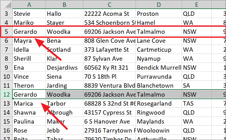
Select the row(s) you want to move the same way we did in the previous sections. Here, we’re selecting row 5.
This time, press and hold the Ctrl key on the keyboard, and drag the row to your desired location using the move pointer. Once you’ve found the right spot for the row, release the mouse click and the Ctrl key. Here, we’re releasing the mouse click at row 12.
Upon releasing the buttons, the 5th-row data replaces the 12th-row data but the 5th-row remains as the original data. Also, there is no pop-up dialog box asking whether to overwrite the data or not.
Move Multiple Rows At A Time by Dragging
You can also move multiple rows at a time using any of the same above methods. However, you can only move contiguous/adjacent rows and you cannot move non-contiguous rows by dragging.
First, select the multiple rows you want to move. You can select the entire multiple rows by clicking and dragging over the row numbers to the left. Alternatively, click on the first or last row header you want to select, press and hold the Shift key and use the arrow keys up or down to select multiple rows. In the example below, we’re selecting from rows 3 to 6.
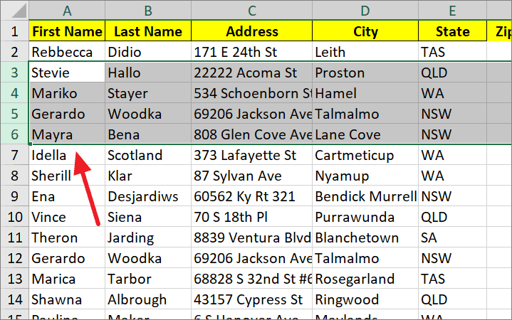
Now, click on the edge of the selection, and drag the rows to the new location. You can simply drag, drag while holding the Shift key, or drag while holding the Ctrl key to move the rows.
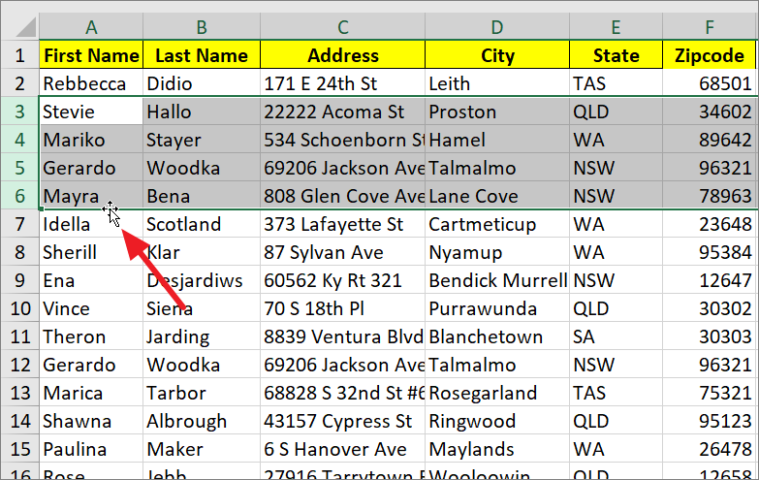
In the example, we’re dragging the rows while holding the Shift key until the bottom line of row 10.
Now, rows 3 to 6 are moved to the location of rows 7 to 10, and the original rows from 7 to 10 are moved/shifted up.
Move Column using Mouse Drag
You can move columns (or contiguous columns) by following the same steps you did for the rows.
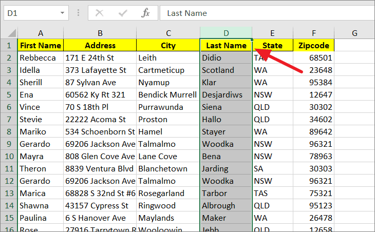
First, select the column (or adjacent columns) that you want to move. You can select an entire column by clicking the column header (column letter) at the top or pressing the Ctrl+Spacebar shortcut keys. In the example, we want column B (Last Name) to come after column D (City), so we’re highlighting column B.
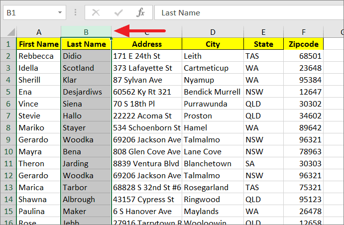
Then, drag the column using Shift + left mouse click and release the mouse button and Shift key when you see the green bold line at the edge between column D and column E.
You can also simply drag the column or hold the Ctrl key while dragging the column to move and replace the existing column.
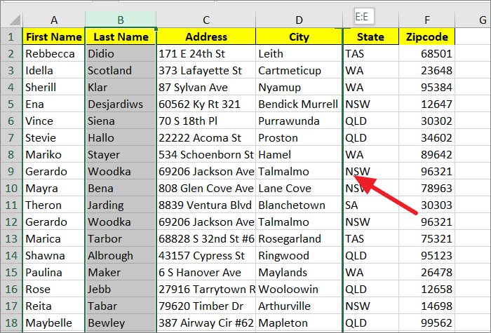
As you can see column B is moved to the location indicated by the bold green border and the original column D (City) is shifted to the left.
Move a Row/Column in Excel With Cut and Paste
Another easiest and well-known method for moving rows in Excel is by cutting and pasting the row of cells from one location to another. You can easily cut and paste rows using shortcut keys or mouse right-click. This method is much more simple and straightforward than the previous method. Let’s see how to move rows using the cut and paste method.
First, select the row (or contiguous rows ) as we did in the previous sections. You can either select an entire row or a range of cells in a row. Then, press the Ctrl+X (Command+X on Mac computer) on your keyboard to cut the selected row from its current location. Alternatively, you can right-click on the selected cell and select ‘Cut’.
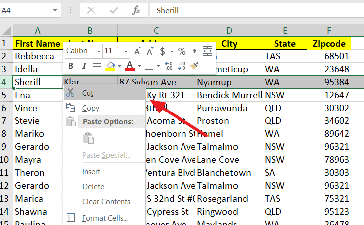
Once you did that, you will see the marching ants effects (moving border of dots) around the row to show it has been cut. In the below example, row 4 is cut.
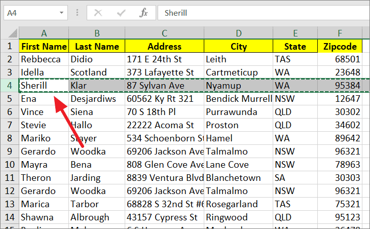
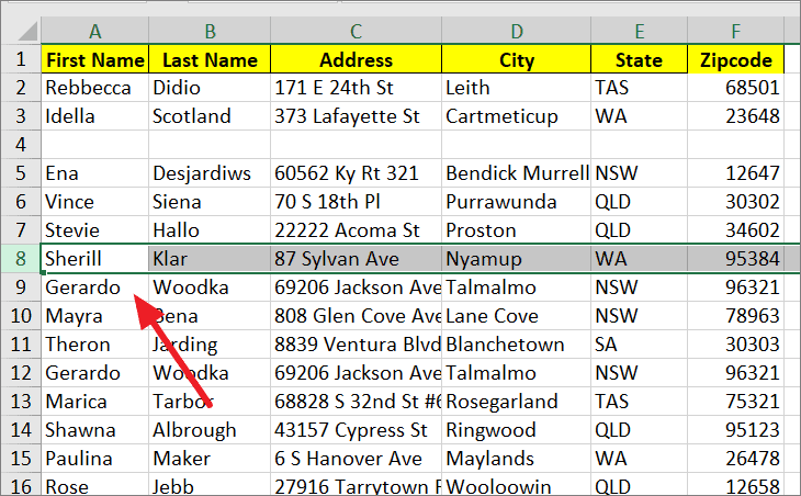
Next, select the desired destination row where you want to paste the cut row. If you moving an entire row, make sure to select the entire destination row by clicking the row number before pasting. Here, we’re selecting row 8.
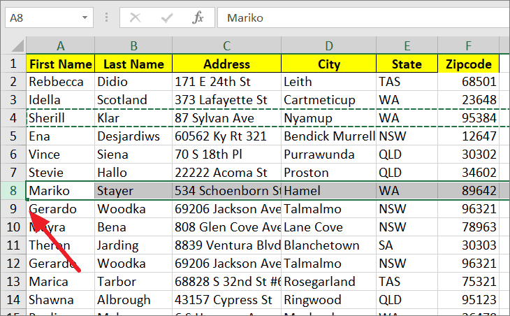
Then, press the Ctrl+V shortcut keys to paste the row or right-click the destination row and click on the ‘Paste’ icon from the context menu.
When you use this method to move rows, it will overwrite the existing row. As you can, the data of row 8 is replaced with the data of row 4 in the below screenshot.
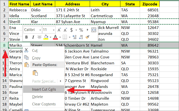
If you don’t want to replace the existing row while moving the selected row, you can use the ‘Insert Cut Cells’ option instead of the simple ‘Paste’ option. Here’s how you do that:
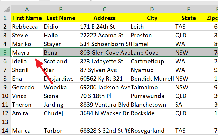
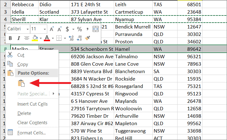
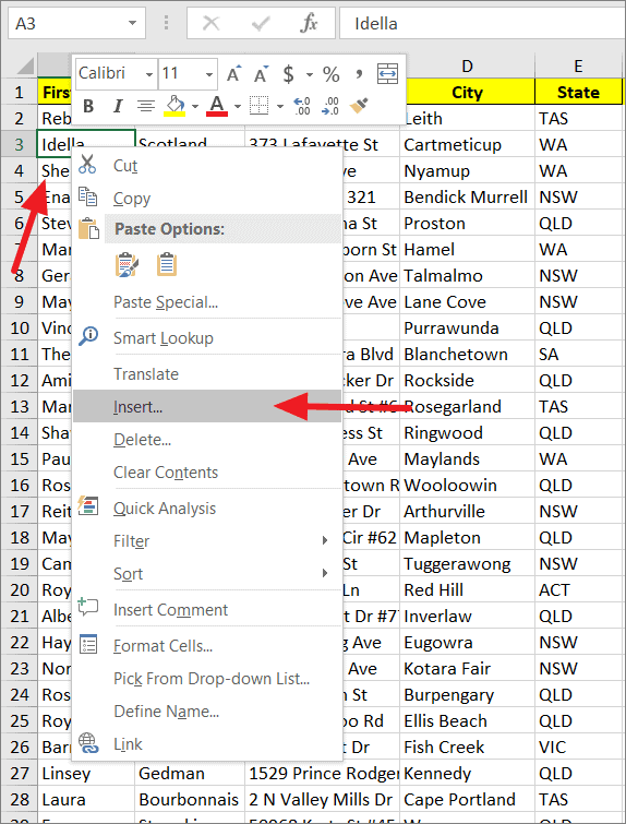
Select the row you want to move, and right-click and select ‘Cut’ or press Ctrl+X. Then, select the row before which you want to insert the cut row, right-click on it and choose ‘Insert Cut Cells’ from the context menu. Alternatively, you can press the Ctrl key + Plus sign (+) key on the numeric keypad to insert the cut row.
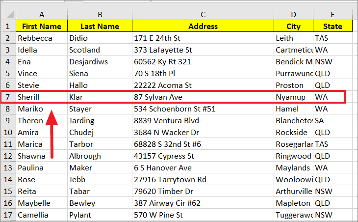
As you can see here, row 4 is inserted above the selected row, and the original row 7 is moved up.
If you want to copy the row rather than cut it, then instead of Ctrl+X, press Ctrl+C to copy the row and press Ctrl+V paste it. You can move columns using the cut and paste method by following these same instructions.
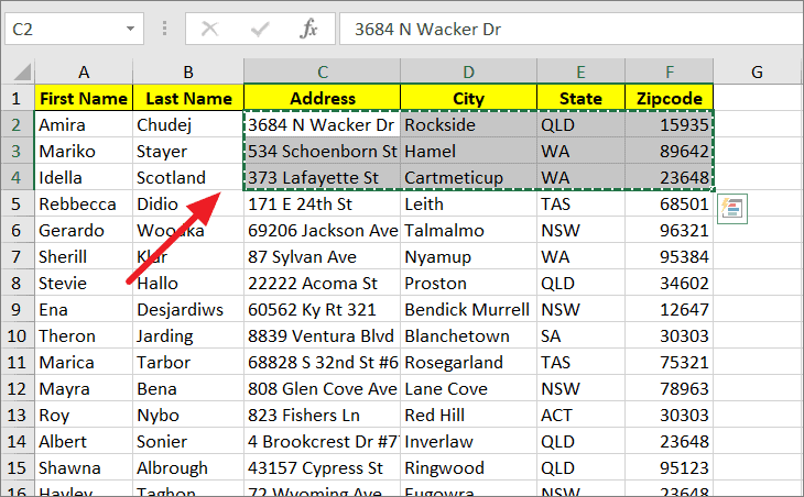
You can also cut a range of cells in a single row or multiple adjacent rows (contiguous rows) instead of entire rows and insert (or paste) them in another location using the above method. For example, we’re cutting C2:F4. Remember, if you are selecting multiple rows in the range, the rows must be adjacent rows.
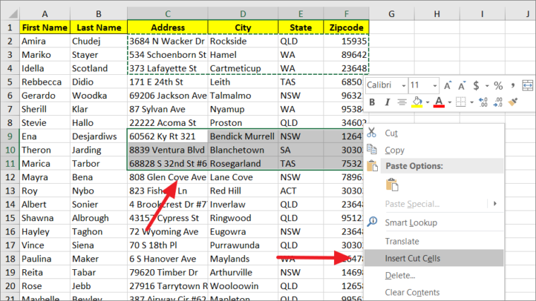
Then, we are pasting the cut rows in the range C9:F11 using the ‘Insert Cut Cells’ option from the right-click menu.
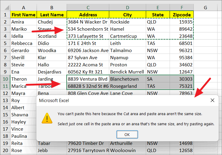
Also, when you are moving rows, the cut area and paste area must be the same size, otherwise, you would get an error when you try to paste the cut row. For example, if you cut rows C2:F4 and try to paste it in the smaller range C10:F11 using the normal paste (Ctrl+V) method, you would see the following error.
Move Rows Using a Data Sort Feature in Excel
Moving rows with the data Sort features may require few more steps than the previous methods, but it is certainly not the difficult method to move rows or columns in Excel. Also, the data sort method comes with an advantage, you can change the order of all rows in one move that includes non-continuous rows as well. This method is certainly useful when it comes to rearranging numerous rows in a large spreadsheet. Follow these steps to move rows using a data sort:
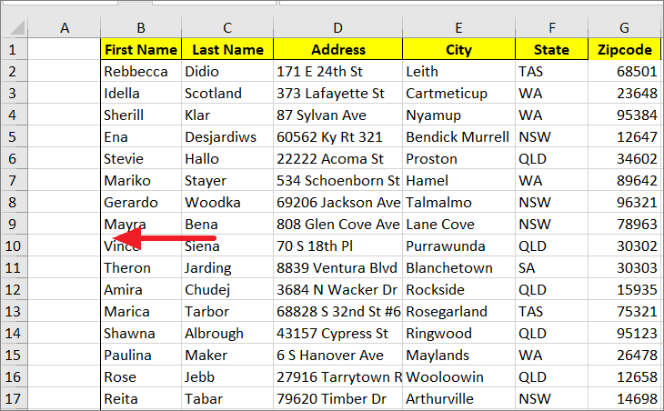
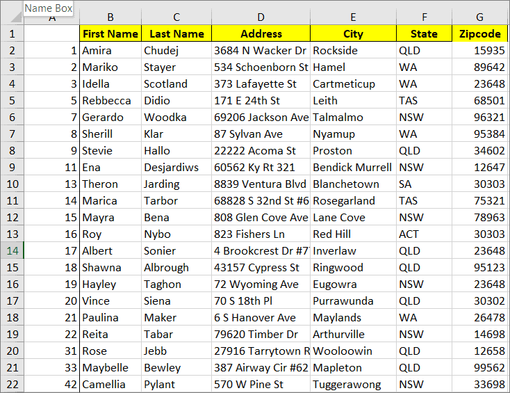
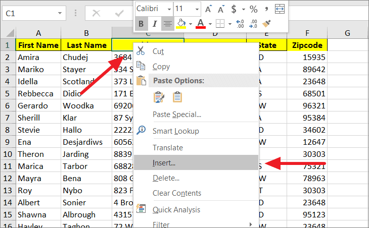
First, you need to add a column to the left-most side of your spreadsheet (column A). To do this, right-click on any cell in the first column and select the ‘Insert’ option from the context menu.
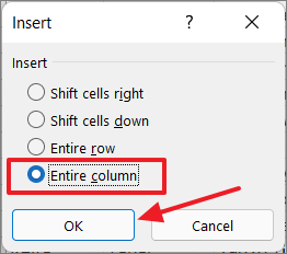
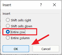
In the Insert pop-up box, select ‘Entire column’ and click ‘OK’.
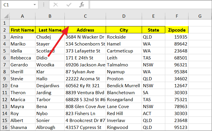
A new column has been inserted to the left-most side of your data set. This column must be the first column of your spreadsheet (i.e. column A).
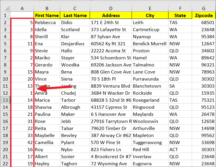
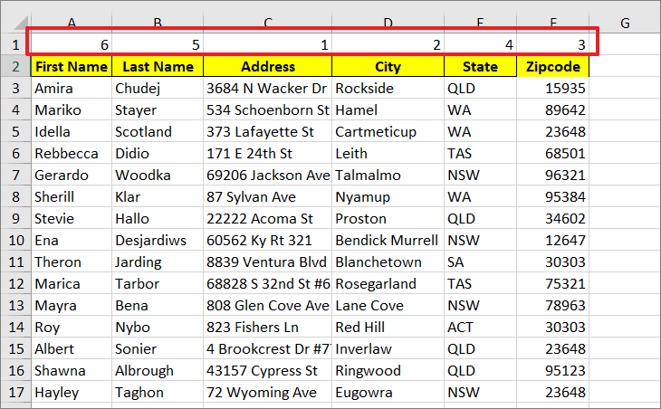
Now, number the rows in the order you want them to appear in your spreadsheet by adding numbers in the first column as shown below.
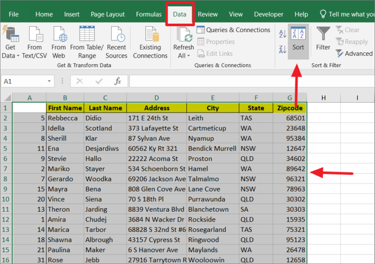
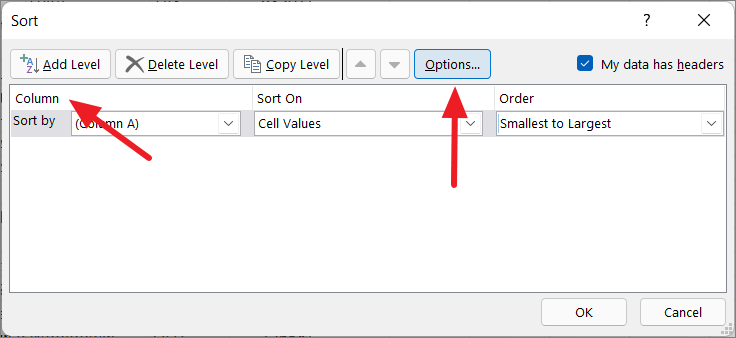
Next, select all the data in the dataset that you want to reorganize. Then, go to the ‘Data’ tab in the Ribbon, and click the ‘Sort’ button in the Sort & Filter group.
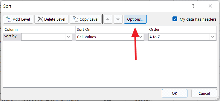
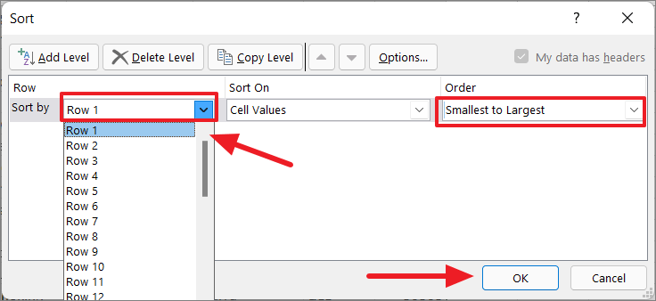
You need to sort the dataset by the numbers in Column A. So, in the Sort dialog box, make sure the sorting is set to ‘Column’ above the ‘Sort by’ drop-down. If not, click the ‘Options’ button at the top.
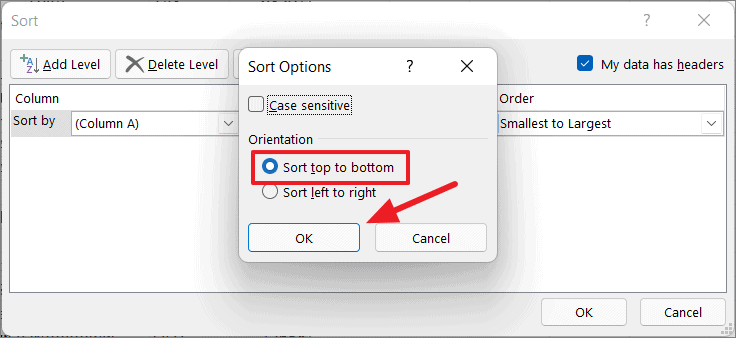
Then, in the Sort Options pop-up dialog, select ‘Sort top to bottom’ and click ‘OK’.
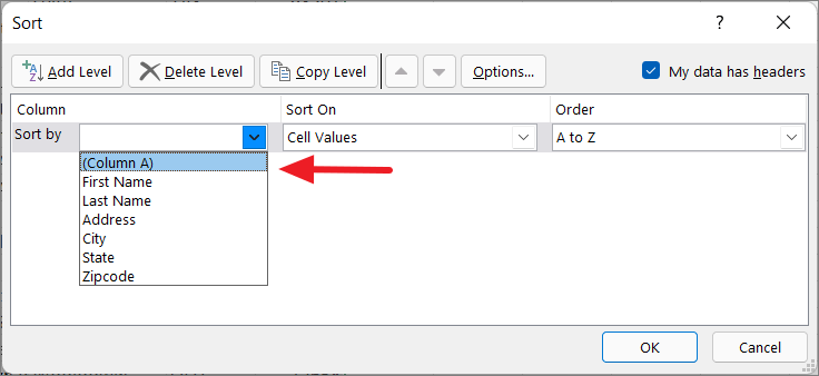
Now, you’ll be back on the Sort dialog window. Here, select ‘Column A’ (or title of your first column) in Sort By drop-down menu.
Then, make sure the ‘Order’ drop-down is set to ‘Smallest to Largest’ and click ‘OK’.
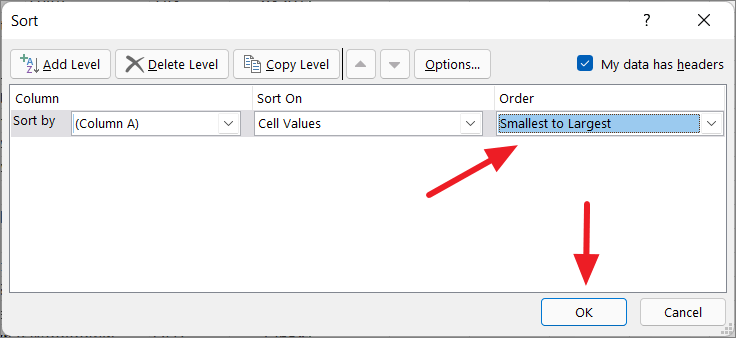
This will close the Sort dialog box and take you back to your spreadsheet, where you’ll find that the rows have been rearranged according to the numbers you listed in that first column. Now, select the first column, right-click and select ‘Delete’ to remove it.
Move Columns Using a Data Sort
The process of moving columns using data sort is essentially the same as the moving rows, with a only few different steps. Follow these steps to move columns using data sort.
To move columns, you need to add a row instead of a column to the top of your dataset (Row 1). To do this, right-click on any cell in the first row and select the ‘Insert’ option from the context menu.
In the Insert dialog box, select ‘Entire row’ this time and click ‘OK’.
A new row will be inserted to the top of your spreadsheet, above all rows of data.
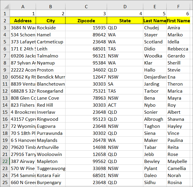
Now, number the columns in the order you want them to appear in your worksheet by adding numbers in the first row as shown below.
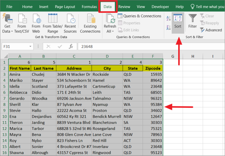
Next, select all the data in the dataset that you want to change the order of. Then, switch to the ‘Data’ tab in the Ribbon, and click the ‘Sort’ in the Sort & Filter group.
Now, you need to sort columns by the numbers in the first row. In the Sort dialog box, you need to set sorting to ‘Row’ instead of the column above the ‘Sort by’ drop-down. To do that, click the ‘Options’ button.
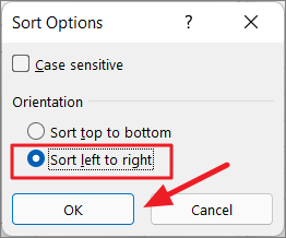
In the Sort Options pop-up dialog box, select ‘Sort left to right’ and click ‘OK’.
Back in the Sort dialog window, select ‘Row 1’ in Sort By drop-down menu and ‘Smallest to Largest’ in the Order drop-down. Then, click ‘OK’.
This will sort (move) the columns based on the numbers you listed in that first row as shown below. Now, all you have to do is select the first row and delete it.
Now, you know everything about moving rows as well as columns in Excel.
Home / Excel Basics / How to Move a Row and Column in Excel
In Excel, sometimes you may need to move a row and column to change its order in the worksheet. It even helps you rectify the errors from the sheet and increase its readability. In this tutorial, we will look at various methods to move a row and column.
You can easily move a row without overwriting on the existing row, press and hold the Shift key.
- Firstly, select the row that you want to move up or down.

- Then, move your cursor to the edge of the row and you will see the icon with four-sided arrows.
- Now, while holding the Shift key and left button of the mouse together drag the selected row to the desired location.
- When you will find the right point for the row, then release the shift key and mouse click.

In the below picture, row 7 is moved to row 5, and the existing row 5 automatically moves down.

Steps to Move a Column
To quickly move a column in Excel use the below steps.
- Select the column first that you want to move in the worksheet.

- Next, hover over the cursor to the border of the selected column and now the four-sided arrow appears there.

- After that, press and hold the Shift key and the mouse left button at once.
- Now, drag the cursor to the new position where you would like to relocate the column.

In the below example, we are observing the Student Section A column is moving in place of Section B.

Move Multiple Rows
If you want to move multiple rows together, you can do it easily, and here, are the steps for this.
- For this, again you have to select all those rows in a sequence that you want to move, and you can select rows by dragging the mouse over them.

- After that, move the mouse pointer to the edge of one of the selected rows.
- Now, you can drag the rows upwards to the point where you want to move them while holding the Shift key.

As you can see that the selected rows 5,6,7 are moved upwards to 2,3,4 and the original rows are shifted down.

Points to Remember
- In the case of multiple rows, you can only move adjacent rows up or down. However, this method is not applied to multiple non-adjacent rows.
- And, without holding the shift key, it will overwrite the rows instead of moving them.
Move Multiple Columns in Excel
To move multiple columns, without overwriting the existing data.
- Select two or more columns by dragging the cursor over the column headers.

- Then, place your cursor on the border of one of the selected columns and now the arrow exists that helps to drag the columns.
- Move the cursor to a new location while holding the Shift key and the left mouse button.

In the below example, the student’s name columns move forward to the subjects.

Move a Row by Cut and Paste
The easiest way to move a row is to use the cut-and-paste method.
- Select the row by its header and then right-click on it and click on the cut option.

- Once you click on it, the row is highlighted in green color.

- Next, click on the row where you want to move this selected row.
- Here, right-click on it and select the Insert cut cells option from the pop-up box.

- Last, you will see the selected row moves up and the original row moves down.


Move a Column by Cut and Paste
- First of all, select the column that you want to move by its header and select the “Cut” option by right-clicking on it.

- You can see now that the column highlights with the green color.

- Now, click on the column where you want to move this and choose the “Insert cut cells” option by right-clicking.

- And, you will see the selected column of section A shift its position, and the students of section B moves to the next column.


Note: By this method, you can even move a row or column to the other sheet on the workbook, by using the insert cut cell option.
Move a Row in Excel (Replace)
- First, select the entire row from the row number that you want to move up.

- After that, place your cursor on the edge of the row header and it would show you an icon with four-sided arrows.
- Next, hold the left button of the mouse and drag the row to the point where you want to move, and it highlights with green color.

- Once you drag the row to another row that has data already, then you will see the pop-up on the window with a question about replacing it.

- Now, when you click OK then it will replace the row and the existing position of the row remain empty.


Move a Column by Replacing
- Select the column that you wish to move to the new position.
- Move your cursor at the border of the column and there you’ll see the four-sided arrow.
- Now, press and hold the left button of the mouse and drag the column by an arrow where you want to place it, and that column highlights with green color.

- If there is already data in the column, then it will ask you to replace it by showing a pop-up.

- When you click the “Ok” button, then it replaces the column, and the previous place of the column remains blank now.


Important: If you are moving a row or column to an empty row, Excel will not display that pop-up box on the window. It will simply move the data to the empty row or column.
How to Move Columns in Excel (and Rows) – Full Tutorial
Knowing how to move rows and columns in Excel is as important as knowing how to copy and paste – it’s essential.
This is something you’d have to do almost all the time while you work in Excel.
So what are you waiting for? Dive into the guide below where we have listed all the possible ways (and shortcuts) to move columns and rows in Excel🚀
Also, to tag along with the guide, download our free sample workbook here.
How to move columns in Excel
There are several ways how you can move or rearrange columns in Excel. Let’s look into each of them below:
Method # 1: Using the Shift key
The first (and the basic) method of moving columns in Excel is by using the Shift key.
How? Look into the example below to understand that.

The data above consists of three columns.
Let’s say we want to move column C between Columns A and B. Here’s how we will do that:
- Select column C by clicking on the column header.

- Hover over the edge of the column and a plus sign appears.
- Hold down the Shift key when you see the plus sign.
- Drag the selected column to the targeted location (before Column B).
Pro Tip!
To move the columns in Excel while keeping the original data intact, we need to use the Shift command all along. This helps you move the columns to the targeted place without disturbing other data.
However, if you try to move the selected column as above using the Control Key, the targeted column will be replaced 🎯
- The final result looks like this.

Column C (Names) is now placed between the column for Order Number and Amount.
Also, note how the column letter has automatically adjusted here (Column C is now Column B). You can do the same for rows in Excel.
If we had tried to do the same without using the Shift key, Excel would have shown a warning prompt 🚩

And the result would look something like this:

The original column B (Amount) is overwritten as we pasted column C in its place.
Method # 2: Using the insert, cut, and paste hack
This method is usually used by Excel newbies. And honestly, it’s not a very sophisticated approach for moving columns. Nevertheless, it works well.
The process is simple. You just select, insert, cut, paste and delete. Bounced over your head?
Don’t worry – we’ve got a detailed explanation below.
Let’s use the same dataset as in the example above. And we again want to move column C between columns A and B, but this time, with a new method.
- Select the destined column (where you want to move Column C).
In our case, it’s column B (Amount).

- Right-click column B and select the Insert option from the drop-down menu.

- A blank column will appear on the left side of the selected column:

- Select column D or press Ctrl + X to cut or CTRL + C to copy the entire column.
Note that after we’ve inserted an additional column before Column B, all columns have moved an alphabet ahead.
The column for Names (previously Column C) has now become Column D 👀
A moving, dotted enclosure will appear around the column. That’s when you’re ready to paste it to the new location.

- Select the header Column B.
- Press down the Control Key + V to paste the column.

- Column D moves between columns A and C (previously Column B) successfully.
Too many steps and a little longer process? That is why this is not the best or the primary method to move columns in Excel.
Method # 3: Using the CTRL key
Just like we can move columns using the Shift key, we can use the Control key for the same purpose too😍
There’s only one difference between both methods. When you copy columns using the CTRL key, the copied data is pasted into a new column. But, and that’s a big BUT – the data in the pasted column is replaced.
Didn’t get it? Let’s understand it through an example below.
We are using the same data as earlier, and we want to move Column C using the Control key this time.
- Select column C by right-clicking the Column C header.

- Press down the Control key and hover over to the edge of the column until you see a plus sign.
- Hold and drag the column to the desired location.
- Column C replaces column B and appears right after the first column.

What happened here was that when we pressed the Control key, Excel made a copy of column C in place of column B by overwriting column B.
You can now delete column C by clicking delete from the context menu.

How to move multiple columns at the same time
Okay, so now you know how to move a column in Excel. But do you know how to move multiple columns simultaneously?
We bet you don’t, and we’re here to teach you just that😎
Let’s say we have this dataset where we want to move columns B and C and bring them before column A.

So, how do we do that? Using the Shift key method as we did previously.
- Select column C by clicking on the header.

- Press down the Shift key and select the header for column B.

- Hover over the edge of Column B until the plus sign appears.
- Hold and drag the columns and drop them before column A.
- The result will look something like this:

Note that this hack works for contiguous columns or contiguous rows only. You cannot use it to move non-contiguous rows and columns in Excel.
Move columns to other worksheets
Now that we know how to work with columns in a single worksheet, it’s time we see how to move them to another sheet in the same workbook.
There’s a small but common hack for moving columns from one sheet to another. Let’s see it here👀
Using the same example as above, we are moving Column A from Sheet 1 to Sheet 3. To do so:
- Create a new sheet from the sheet tab at the bottom by clicking on the + sign shown below.

- Navigate back to Sheet 1.
- Select column A and press CTRL + C if you want to keep a copy of the column in Sheet 1. Otherwise, press CTRL + X to cut the column.

- Go to Sheet 3.
- Paste the contents in any column of Sheet 3 by selecting it and pressing CTRL + V.
For example, we’ve pasted it in Column A of Sheet 3 as shown below.

How to move rows in Excel
We now know how to work with columns in Excel. Let’s see a brief overview of moving rows in an Excel spreadsheet too.
Method # 1: Using the Shift key
This one’s easy. Simply select the row you want to move, press shift, and drag it to the new position.
Let’s see an example here:

In the dataset above, the 6th row comes in the wrong order. It should have been in the first position (Row 2).
No worries – let’s move it to the right place. For that:
- Select the relevant row number (in our case, row 6).

- Hover over the edge of the row until the plus sign appears.
- Press down the Shift key and drag the entire row to its new location.
- The selected row moves up, and the result looks like this:

You can do the same for multiple rows by selecting them at once and dragging them to the new position.
Method # 2: Using the insert, cut, and paste hack to move rows
You know this one already, don’t you? It’s an easy hack, and you just need to follow the same steps as with columns.
- Select the new row where you want the previous row to be moved. In this case, we want to move row 5 above row 9.

- Once selected, open the context menu with a right-click.
- Select the Insert option to add a single row.

- A new blank row appears above the 9th row.

- Cut row 5 by selecting it and pressing the Control key + X.

- Go to Row 9 (the newly inserted blank row).
- Paste Column 5 in there by pressing Control + V.

Now that all the data is organized, we have an empty row (Row 5) in our dataset.
You might want to delete it as follows:
- Select row 5 and right-click on it to launch the context menu.
- From the context menu, choose the Delete option to delete the subject row.

- This is what your dataset looks like now:

Method#3: Using the CTRL Key
You can also rearrange rows using the Control key. The method is identical to how we moved columns using the Control key.
Let’s quickly reiterate it here for moving rows:
- Select the row to be moved.
- Press and hold down the Control key.
- Hover over the row until you see a plus sign.
- Drag the row to its new position.
- The new row will appear, and the previous row will be replaced.
That’s it – Now what?
In this article, we learned easy hacks to move columns and rows in Excel using Shift, CTRL, and the Insert method🔰
But there is so much more you can do with columns and rows in Excel. And this article doesn’t do justice in covering even 5% of that information.
There are tons of other things to Excel that you’d want to learn. And you can start by practicing with some core Excel functions like the VLOOKUP, IF, and SUMIF functions.
Enroll in my 30 minutes free email course today to learn these functions (and more!).
Kasper Langmann2022-12-27T03:25:45+00:00
Page load link
Move or copy rows and columns by using the mouse Select the row or column that you want to move or copy. , drag the rows or columns to another location. , drag the rows or columns to another location. Important: Make sure that you hold down CTRL during the drag-and-drop operation.
Contents
- 1 How do I move rows to scroll in Excel?
- 2 How do you move cells up in Excel?
- 3 How do I scroll rows and rows in Excel?
- 4 How do I swap rows in Excel?
- 5 How do you scroll down in Excel without moving the top row?
- 6 How do you move down a line in Excel within a cell?
- 7 What is the Scroll Lock key?
- 8 How do I move all cells up?
- 9 How do you shift all cells down?
- 10 Why is Excel scrolling with arrow keys?
- 11 How do you switch rows and columns in Excel table?
- 12 How do you swap rows in sheets?
- 13 How do I scroll first row in Excel?
- 14 How do I keep a chart in view when scrolling in Excel?
- 15 How do you hit enter and stay in the same cell?
- 16 What is Ctrl enter in Excel?
- 17 How do you insert a row within a cell in Excel?
- 18 How do I unlock Scroll Lock in Excel?
- 19 Can’t scroll down Excel?
- 20 How do you unlock Scroll Lock in Excel shortcut?
How do I move rows to scroll in Excel?
Click the View tab on the Ribbon. Select the Freeze Panes command, then choose Freeze Panes from the drop-down menu. The rows will be frozen in place, as indicated by the gray line. You can scroll down the worksheet while continuing to view the frozen rows at the top.
How do you move cells up in Excel?
Move cells by drag and dropping
- Select the cells or range of cells that you want to move or copy.
- Point to the border of the selection.
- When the pointer becomes a move pointer. , drag the cell or range of cells to another location.
How do I scroll rows and rows in Excel?
To scroll one column or row at a time in a particular direction, click the appropriate scroll arrow at the ends of the scroll bar. For example, to scroll right one column, click the arrow on the right side of the horizontal scroll bar.
How do I swap rows in Excel?
Hover your mouse over the border between the two adjacent rows until it turns into a cross-arrow icon. Click and hold your mouse and “Shift” until you see a gray line appear under the row you want to switch the data with. Let go of the mouse button, and the data will switch places.
How do you scroll down in Excel without moving the top row?
Select the cell in the upper-left corner of the range you want to remain scrollable.
To freeze the top row or first column:
- From the View tab, Windows Group, click the Freeze Panes drop down arrow.
- Select either Freeze Top Row or Freeze First Column.
- Excel inserts a thin line to show you where the frozen pane begins.
How do you move down a line in Excel within a cell?
Microsoft Excel in Windows
On all versions of Microsoft Excel for the PC and Windows, the keyboard shortcut Alt + Enter moves to the next line. To use this keyboard shortcut, type text in the cell and when ready for a new line, press and hold down the Alt key, then press the Enter key.
What is the Scroll Lock key?
On PC keyboards, a key used to toggle between a scrolling and non-scrolling mode. When on, the Arrow keys scroll the screen regardless of the current cursor location. This key is rarely used for its intended purpose, if at all. See PC keyboard.
How do I move all cells up?
Select the cell or cell range you want to move. Move the mouse pointer over the outline of the selected cells. Click and drag the cells to the new location.
How do you shift all cells down?
Open a Spreadsheet
- Open a Spreadsheet.
- Launch Excel and open your spreadsheet using the File menu and “Open” prompt.
- Click a Cell in the Row to Shift Downward.
- Click on any cell in the highest row that you want to shift downward.
- Select “Insert Sheet Rows”
- Click the “Home” tab if it is not already selected by default.
Why is Excel scrolling with arrow keys?
When the scroll lock feature is turned on, pressing an arrow key causes Microsoft Excel to move the entire spreadsheet, instead of moving to the next cell. Although helpful for a user viewing a large worksheet, it’s also quite annoying for those who have mistakenly enabled this feature.
How do you switch rows and columns in Excel table?
Transpose (rotate) data from rows to columns or vice versa
- Select the range of data you want to rearrange, including any row or column labels, and press Ctrl+C.
- Choose a new location in the worksheet where you want to paste the transposed table, ensuring that there is plenty of room to paste your data.
How do you swap rows in sheets?
Move rows or columns
- On your computer, open a spreadsheet in Google Sheets.
- Select the rows or columns to move.
- At the top, click Edit.
- Select the direction you want to move the row or column, like Move row up.
How do I scroll first row in Excel?
How to freeze the top row in Excel
- Scroll your spreadsheet until the row you want to lock in place is the first row visible under the row of letters.
- In the menu, click “View.”
- In the ribbon, click “Freeze Panes” and then click “Freeze Top Row.”
How do I keep a chart in view when scrolling in Excel?
How to always keep a chart in view when scrolling in Excel?
- Right click at sheet tab that you want to keep the chart visible, and click View Code form the context menu. See screenshot:
- Save and close the dialog, then the chart will be moved down or up as you clicking at any cell.
How do you hit enter and stay in the same cell?
Stay in the same cell after pressing the Enter key with Shortcut Keys. In Excel, you can also use shortcut keys to solve this task. After entering the content, please press Ctrl + Enter keys together instead of just Enter key, and you can see the entered cell is still selected.
What is Ctrl enter in Excel?
#2 – Ctrl+Enter to Fill All Selected Cells with the Same Data or Formula. When we are entering data or a formula in a cell, and have multiple cells selected, Ctrl+Enter will copy the data/formula to all of the selected cells.
How do you insert a row within a cell in Excel?
Insert or delete a row
- Select any cell within the row, then go to Home > Insert > Insert Sheet Rows or Delete Sheet Rows.
- Alternatively, right-click the row number, and then select Insert or Delete.
How do I unlock Scroll Lock in Excel?
Click Change PC Settings. Select Ease of Access > Keyboard. Click the On Screen Keyboard slider button to turn it on. When the on-screen keyboard appears on your screen, click the ScrLk button.
Can’t scroll down Excel?
In most cases, users can’t scroll down Excel spreadsheets because there are frozen panes within them. To unfreeze panes in Excel, select the View tab. Click the Freeze Panes button. Then select the Unfreeze panes option.
How do you unlock Scroll Lock in Excel shortcut?
To turn off scroll lock, execute the following step(s).
- Press the Scroll Lock key (Scroll Lock or ScrLk) on your keyboard.
- Click Start > Settings > Ease of Access > Keyboard > Use the On-Screen Keyboard (or press the Windows logo key + CTRL + O).
- Click the ScrLk button.
In simple terms, moving the rows and columns in Excel is just the matter of cut and paste or pressing the short keys Ctrl + X and Ctrl + V, that you might already use to while working in Excel, MS Word or other programs.
However, you may move columns and rows in other ways as well. In this tutorial, I will show you how to move columns and rows in Excel by copy/paste and another way with demo pictures – so keep reading.
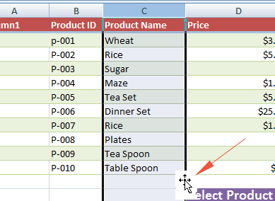
Moving column by mouse drag
Follow these steps for moving a column to the desired location by using the mouse.
Step 1:
Select a column by clicking on A, B, C etc.
Step 2:
Bring to mouse over the border of any cell in of the selected column so that mouse pointer becomes move pointer:
![]()
The picture below shows border with move pointer:
Step 3:
Drag the move pointer to the desired location where you want to relocate the column. For example, we want to move the column C to the H:
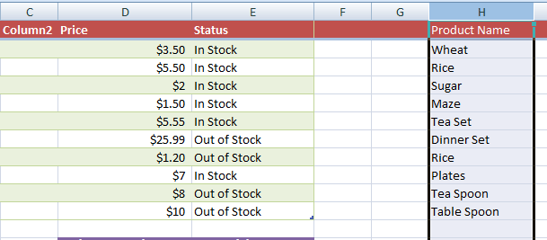
You can see the C column is moved to the H.
Note that, this method cut/pastes the column to the new location. If you want to copy the column to the new location while keeping existing in place then just press the Ctrl key before dragging the column to the new location.
Moving column by short keys
For moving a column by short key, follow this:
Step 1:
Select the column as we did in the above example. For example, we selected C in our demo.
Step 2:
Press the Ctrl + X on Windows or Command + X on Mac operating system.
Step 3:
Select the desired destination column letter that will highlight the whole column. In our demo, we selected H.
Now press Ctrl + V on Windows OS or Command + V on Mac.
Using Mouse Right Click
Step 1:
Select a column header as we did in both above methods. I selected C column again that I will move to column H.
Step 2:
From the keyboard, press Ctrl + X on Windows or Command + X on Mac OS. This should make the borders of C column dotted.
Step 3:
Select column H header so that whole column is selected and press Ctrl + V (Windows) or Command + V on Mac.
This will move the contents of column C to column H.
If you want to copy the content rather than cut/paste then instead of Ctrl + X in step 2, press Ctrl + C or Command + C short keys.
A word of caution before moving ahead
As moving columns, Excel copies the content as well as any formulas, resulting in moving the values, hidden cells, and cell formats.
However, cell references are not adjusted. You need to adjust the column references manually.
For example, as we moved C column contents to H and if other cells like D column cells are referencing the C cells then those will keep on referencing C after you copied the content to H. That may result in #REF! error – so be careful.
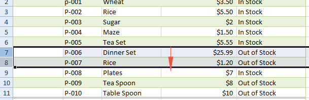
Moving rows example
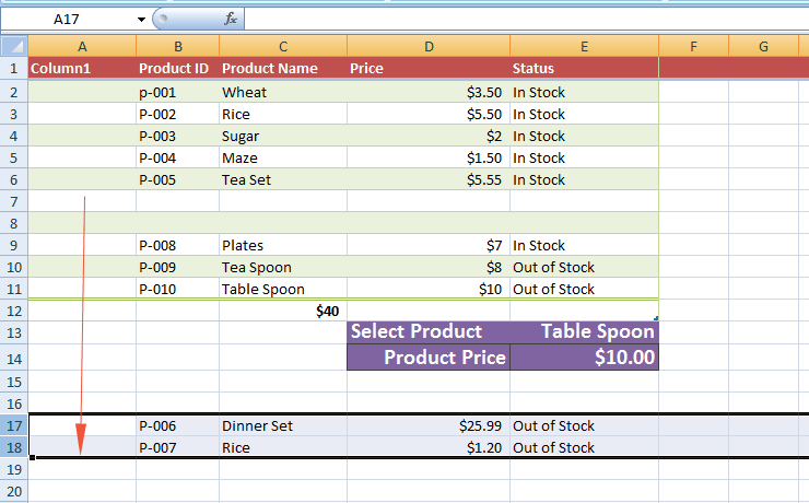
For moving one or more rows, the procedure is almost the same as in the case of columns. Follow these steps for moving one or more rows to a new location. We will move row number 7 and 8 to the 17 and 18.
Step 1:
Select a row by clicking on the number towards the left side. If you want to select more than one row then keep on selecting the rows by first pressing on a number and then move up or down as mouse is pressed.
You may also use the Shift key after selecting the first row with mouse and then press the Shift + Down or Up arrow.
For example, I selected 7 and 8 as shown below:
Step 2:
Bring the mouse over the black thick border so that move pointer displays.
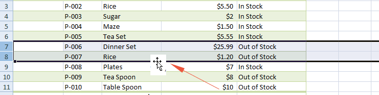
Step 3:
Drag the mouse towards down and leave it at row 17 (for our demo). You will leave it to the destination row as required.
Using short keys for moving rows
You may also use keyboard shortcut keys for moving the rows.
Step 1:
Select the rows that you want to move as in the above case. I selected 7 and 8 row.
Step 2:
Press Ctrl + X (Windows) or Command + X (Mac users).
Step 3:
Go to the first cell of 17 row i.e. A17 (for our demo) and press Ctrl + V or Command + V.
That’s it!
Sometimes you need to reorder columns or rows in Excel. If your data does not contain formulas, the procedure does not seem complicated – copy/paste works well for the plain data cells. However, when you try to move data with formulas, you may run into problems.
There are two ways how you can move or rearrange an entire column or row in Excel:
- Using the keyboard or ribbon:
1. Insert an empty column (or row) where you want to insert the moved one:
1.1. Select a column or row before which you want to insert the moved column (or row) by clicking on the header or pressing Ctrl+Space for selecting the entire column (Shift+Space for selecting the entire row):

1.2. Do one of the following:
- Right-click on the header and choose Insert from the popup menu:

- On the Home tab, in the Cells group, click the Insert drop-down list. Then click Insert Sheet Columns (or Insert Sheet Rows):


2. Copy the moved column or row to the clipboard by clicking on the Cut button in the Clipboard group on the Home tab or by pressing Ctrl+X:

Excel marks the cut item with the dashed line. For example, the entire column is surrounded by the dashed line:

3. Paste moved data into the inserted empty column or row:
3.1. Select the empty column or row.
3.2. On the Home tab, in the Clipboard group, click the Paste button or press Ctrl+V:

Excel inserts the new column and removes the old one. For example, the entire column:

Note: For the plain data, you can use the Copy (Ctrl+C) instead of Cut (Ctrl+X) and remove the source column later. However, if you have formulas in the moved cells, you need to use the Cut function to keep all the references.
- Using the mouse:
You can simply reorder Excel columns or rows by drag-and-drop their headers. To move rows or columns, do the following:
1. Press and hold the Shift key.
Note: If you don’t press and hold the Shift key, the data is replaced by dragging. You can press and hold the Ctrl key to copy the moved data instead of the existing data where you release the move.
2. Point to the border of the selection. When the pointer becomes a Move Pointer ![]() , drag the rows or columns to another location. For example:
, drag the rows or columns to another location. For example:
