
Move or copy cells and cell contents
Use Cut, Copy, and Paste to move or copy cell contents. Or copy specific contents or attributes from the cells. For example, copy the resulting value of a formula without copying the formula, or copy only the formula.
When you move or copy a cell, Excel moves or copies the cell, including formulas and their resulting values, cell formats, and comments.
You can move cells in Excel by drag and dropping or using the Cut and Paste commands.

Move cells by drag and dropping
-
Select the cells or range of cells that you want to move or copy.
-
Point to the border of the selection.
-
When the pointer becomes a move pointer
 , drag the cell or range of cells to another location.
Move cells by using Cut and Paste
-
Select a cell or a cell range.
-
Select Home > Cut
or press Ctrl + X. -
Select a cell where you want to move the data.
-
Select Home > Paste
or press Ctrl + V.
Copy cells by using Copy and Paste
-
Select the cell or range of cells.
-
Select Copy or press Ctrl + C.
-
Select Paste or press Ctrl + V.
Need more help?
You can always ask an expert in the Excel Tech Community or get support in the Answers community.
See Also
Move or copy cells, rows, and columns
Need more help?
Содержание
- Move or copy cells and cell contents
- Need more help?
- Move or copy cells and cell contents
- Need more help?
- Move or copy cells, rows, and columns
- Excel – Go To Cell, Row, or Column Shortcuts
- Go To and Select Cell
- Go To and Select Row
- Go To and Select Column
- Go To a Cell on a Different Sheet
- Go To Named Range or Table
- Move to a Cell With the Name Box
- Move to a Row or Column With the Name Box
- Move to a Named Range or Table With the Name Box
- Move Around the Worksheet With Home and Arrow Keys
- Move Between Formulas – Precedents and Dependents
- Select and Move to Precedent Cells
- Select and Move to Dependent Cells
- Move Around a Workbook with Hyperlinks
- Move to a Row in Google Sheets
- Summary of Shortcuts
Move or copy cells and cell contents
Use Cut, Copy, and Paste to move or copy cell contents. Or copy specific contents or attributes from the cells. For example, copy the resulting value of a formula without copying the formula, or copy only the formula.
When you move or copy a cell, Excel moves or copies the cell, including formulas and their resulting values, cell formats, and comments.
You can move cells in Excel by drag and dropping or using the Cut and Paste commands.
Move cells by drag and dropping
Select the cells or range of cells that you want to move or copy.
Point to the border of the selection.
When the pointer becomes a move pointer  , drag the cell or range of cells to another location.
Move cells by using Cut and Paste
Select a cell or a cell range.
Select Home > Cut  or press Ctrl + X.
Select a cell where you want to move the data.
Select Home > Paste  or press Ctrl + V.
Copy cells by using Copy and Paste
Select the cell or range of cells.
Select Copy or press Ctrl + C.
Select Paste or press Ctrl + V.
Need more help?
You can always ask an expert in the Excel Tech Community or get support in the Answers community.
Источник
Move or copy cells and cell contents
Use Cut, Copy, and Paste to move or copy cell contents. Or copy specific contents or attributes from the cells. For example, copy the resulting value of a formula without copying the formula, or copy only the formula.
When you move or copy a cell, Excel moves or copies the cell, including formulas and their resulting values, cell formats, and comments.
You can move cells in Excel by drag and dropping or using the Cut and Paste commands.
Move cells by drag and dropping
Select the cells or range of cells that you want to move or copy.
Point to the border of the selection.
When the pointer becomes a move pointer , drag the cell or range of cells to another location.
Move cells by using Cut and Paste
Select a cell or a cell range.
Select Home > Cut or press Ctrl + X.
Select a cell where you want to move the data.
Select Home > Paste or press Ctrl + V.
Copy cells by using Copy and Paste
Select the cell or range of cells.
Select Copy or press Ctrl + C.
Select Paste or press Ctrl + V.
Need more help?
You can always ask an expert in the Excel Tech Community or get support in the Answers community.
Источник
Move or copy cells, rows, and columns
When you move or copy rows and columns, by default Excel moves or copies all data that they contain, including formulas and their resulting values, comments, cell formats, and hidden cells.
When you copy cells that contain a formula, the relative cell references are not adjusted. Therefore, the contents of cells and of any cells that point to them might display the #REF! error value. If that happens, you can adjust the references manually. For more information, see Detect errors in formulas.
You can use the Cut command or Copy command to move or copy selected cells, rows, and columns, but you can also move or copy them by using the mouse.
By default, Excel displays the Paste Options button. If you need to redisplay it, go to Advanced in Excel Options. For more information, see Advanced options.
Select the cell, row, or column that you want to move or copy.
Do one of the following:
To move rows or columns, on the Home tab, in the Clipboard group, click Cut  or press CTRL+X.
To copy rows or columns, on the Home tab, in the Clipboard group, click Copy  or press CTRL+C.
Right-click a row or column below or to the right of where you want to move or copy your selection, and then do one of the following:
When you are moving rows or columns, click Insert Cut Cells.
When you are copying rows or columns, click Insert Copied Cells.
Tip: To move or copy a selection to a different worksheet or workbook, click another worksheet tab or switch to another workbook, and then select the upper-left cell of the paste area.
Note: Excel displays an animated moving border around cells that were cut or copied. To cancel a moving border, press Esc.
By default, drag-and-drop editing is turned on so that you can use the mouse to move and copy cells.
Select the row or column that you want to move or copy.
Do one of the following:
Cut and replace Point to the border of the selection. When the pointer becomes a move pointer  , drag the rows or columns to another location. Excel warns you if you are going to replace a column. Press Cancel to avoid replacing.
Copy and replace Hold down CTRL while you point to the border of the selection. When the pointer becomes a copy pointer  , drag the rows or columns to another location. Excel doesn’t warn you if you are going to replace a column. Press CTRL+Z if you don’t want to replace a row or column.
Cut and insert Hold down SHIFT while you point to the border of the selection. When the pointer becomes a move pointer , drag the rows or columns to another location.
Copy and insert Hold down SHIFT and CTRL while you point to the border of the selection. When the pointer becomes a move pointer , drag the rows or columns to another location.
Note: Make sure that you hold down CTRL or SHIFT during the drag-and-drop operation. If you release CTRL or SHIFT before you release the mouse button, you will move the rows or columns instead of copying them.
Note: You cannot move or copy nonadjacent rows and columns by using the mouse.
Источник
Excel – Go To Cell, Row, or Column Shortcuts
This tutorial demonstrates how to go to a specific cell, column, or row using keyboard shortcuts in Excel.
Go To and Select Cell
In Excel, you can easily move from one selected cell to another using the Go To option. Say you have cell A1 selected and want to move to cell C3.
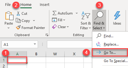
- Select any cell (e.g., A1), and in the Ribbon, navigate to Home > Find & Select > Go To (or use the keyboard shortcut CTRL + G).
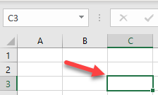
- In the Go To window, enter the cell you want to move to (e.g., C3) in the Reference box and click OK.
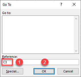
As a result, you moved from cell A1 to cell C3, which is now selected.
Go To and Select Row
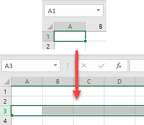
Just as with a cell, you can also move to and select an entire row using the Go To feature. This time, say you want to move from cell A1 and select Row 3. To achieve this, follow Step 1 from the previous section.
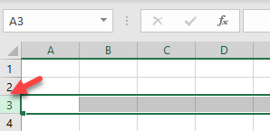
In the Go To window, enter the row you want to move to in the format row:row (e.g., 3:3) in the Reference box and click OK.
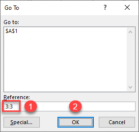
This moves you from cell A1 to Row 3, which is now selected in its entirety.
Go To and Select Column
Moving to a specific column follows exactly the same procedure.
In the Go To window, enter the row you want to move to in the format column:column (e.g., D:D) in the Reference box and click OK.
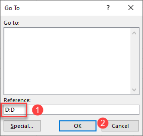
This moves you from your current cell to Column D, which is selected in its entirety.
Go To a Cell on a Different Sheet
To move to a cell on a different sheet, type the sheet name into the Go To window.
In the Go To window, enter the row you want to move to in the format sheetname!cell (e.g., Sheet3!A5) in the Reference box and click OK.
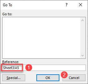
This moves you to the specified cell in the specified sheet.
Note: The sheet name has to have an exclamation mark (!) after it to indicate that it is a sheet.
Go To Named Range or Table
You can also use the Go To window to move to any range names or tables that have been created in your workbook.
In the Go To window, click on the range name or table in the Reference box and click OK.
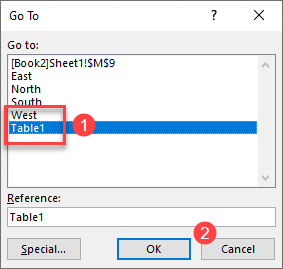
Your range name or table is selected.
Move to a Cell With the Name Box
You can also move to a cell using the name box. The name box is positioned to the left of the formula bar and shows the name of a selected range.
- To move from A1 to C3, first select cell A1.
- Then in the name box, type C3 and press ENTER.
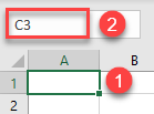
The result is the same as with the Go To option, and cell C3 is selected.
Move to a Row or Column With the Name Box
Just like in the previous section, you can move to a specific row with the name box.
- To move from cell A1, and select entire Row 3, select A1.
- Then in the name box, type 3:3 to move to Row 3, or D:D to move to Column D and press ENTER.
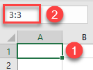
Again, the entire Row 3 or Column D is selected.
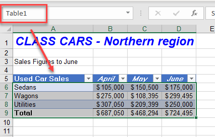
Move to a Named Range or Table With the Name Box
To move to a range name or table using the name box, type in the range or table name, and then press ENTER.
The entire named range or table is selected.
Move Around the Worksheet With Home and Arrow Keys
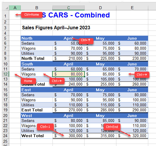
The first cell in a worksheet is always cell A1. To move there quickly using they keyboard, press CTRL + HOME.
To move to the last occupied cell in a worksheet, press CTRL + END.
To move to the first cell in the currently selected row, press HOME.
Moving to the first cell of a column is a bit more complicated! Press CTRL + ↑ (up arrow) (or END > ↑) to move up to the last cell used in a column above your currently selected position. You can then press CTRL + ↑ to move up to the last used cell in the range of cells you have moved to. You can continue pressing CTRL + ↑ until you move to the top of your column.
You can also use the other arrow keys to move around the worksheet.
- CTRL + → (right arrow) (or END > →) moves you to the last cell that is populated in the current row or, if no more cells are populated after your currently selected cell, it moves you to the last cell in the row completely.
- CTRL + ← (left arrow) (or END > ←) moves you to the first cell that is populated in the current row, or if all the cells are populated before the current position, it moves you to column 1 in the current row.
- CTRL + ↓ (down arrow) (or END > ↓) moves you to the last cell that is populated in the current column below your current position, or if all the cells are populated above your current position, it moves you down the last cell in the worksheet.
- CTRL + ↑ moves you up to the last cell that is populated in the current column if you are below it, or if all the cells above your current position are populated, it moves you up to Row 1.
Note: Don’t hold the END key down as you do the CTRL key. Press the END key first, and then the relevant arrow key).
Move Between Formulas – Precedents and Dependents
You can use CTRL + ] (close bracket) or CTRL + [ (open bracket) to move between cells with formulas that are linked to each other.
Select and Move to Precedent Cells
You can select and move to a cell’s precedents by using the CTRL + [ (open bracket) shortcut.
Say you have a worksheet that has a sum formula such as the example below.
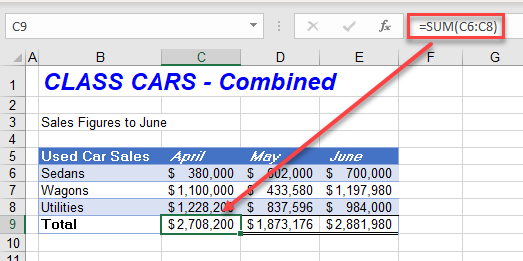
Click on the cell that contains the formula and then press CTRL + [ on the keyboard.
All cells that are referenced in the formula – the cell’s precedents – are selected.
If the formula just refers to one cell, CTRL + [ moves to the specific precedent cell referenced in the formula.
- Click on the cell that contains the formula.
- Press CTRL + [ to move to the cell referenced in the formula.
Select and Move to Dependent Cells
You can also jump to a formula that is a dependent of your selected cell by using the CTRL + ] (close bracket) shortcut.
If the selected cell is used in a formula in another cell, and you press CTRL + ], you automatically jump to the cell that contains the formula.
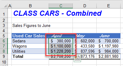
Say for example, you have the following cell selected.
If you press CTRL + ], you automatically jump to the cell that contains the formula. (If the cell is referenced in multiple formulas, all dependent cells are selected at once.)
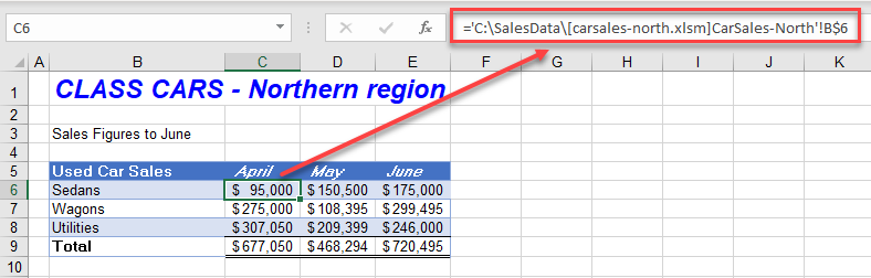
If you click on a formula that refers to a different workbook and press CTRL + ], you automatically jump to the cell within that workbook. If the workbook is not open, then Excel automatically opens it for you.
Move Around a Workbook with Hyperlinks
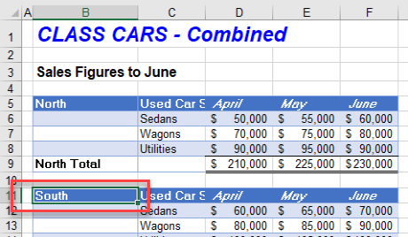
You can create hyperlinks within a workbook to move around.
Click in the cell where you wish the hyperlink to go.
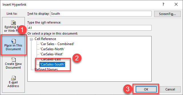
- Press CTRL + K on the keyboard and then select Place in This Document.
- Next, select the sheet where you wish the hyperlink to jump to.
- Click OK.
This creates a hyperlink. Click on it to go to the selected reference.
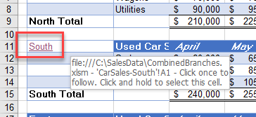
Note that when you hover over the cell, the entire cell path and filename are shown, even though the linked cell is in the same file.
Move to a Row in Google Sheets
Google Sheets doesn’t have “Go To,” but you can use the name box to move to a cell or row. It works exactly the same way as it does in Excel. You can also use the CTRL, HOME, END, and arrow keys to move around your worksheet.
Click in the name box and type in the cell address of the cell you wish to navigate to, and then press ENTER to move to that cell.
Summary of Shortcuts
Here’s a list of the shortcuts discussed above. For more keyboard shortcuts, see Excel Shortcuts List for Mac and PC.
Источник
This tutorial demonstrates how to go to a specific cell, column, or row using keyboard shortcuts in Excel.
Go To and Select Cell
In Excel, you can easily move from one selected cell to another using the Go To option. Say you have cell A1 selected and want to move to cell C3.
- Select any cell (e.g., A1), and in the Ribbon, navigate to Home > Find & Select > Go To (or use the keyboard shortcut CTRL + G).
- In the Go To window, enter the cell you want to move to (e.g., C3) in the Reference box and click OK.
As a result, you moved from cell A1 to cell C3, which is now selected.
Go To and Select Row
Just as with a cell, you can also move to and select an entire row using the Go To feature. This time, say you want to move from cell A1 and select Row 3. To achieve this, follow Step 1 from the previous section.
In the Go To window, enter the row you want to move to in the format row:row (e.g., 3:3) in the Reference box and click OK.
This moves you from cell A1 to Row 3, which is now selected in its entirety.
Go To and Select Column
Moving to a specific column follows exactly the same procedure.
In the Go To window, enter the row you want to move to in the format column:column (e.g., D:D) in the Reference box and click OK.
This moves you from your current cell to Column D, which is selected in its entirety.
Go To a Cell on a Different Sheet
To move to a cell on a different sheet, type the sheet name into the Go To window.
In the Go To window, enter the row you want to move to in the format sheetname!cell (e.g., Sheet3!A5) in the Reference box and click OK.
This moves you to the specified cell in the specified sheet.
Note: The sheet name has to have an exclamation mark (!) after it to indicate that it is a sheet.
Go To Named Range or Table
You can also use the Go To window to move to any range names or tables that have been created in your workbook.
In the Go To window, click on the range name or table in the Reference box and click OK.
Your range name or table is selected.
Move to a Cell With the Name Box
You can also move to a cell using the name box. The name box is positioned to the left of the formula bar and shows the name of a selected range.
- To move from A1 to C3, first select cell A1.
- Then in the name box, type C3 and press ENTER.
The result is the same as with the Go To option, and cell C3 is selected.
Move to a Row or Column With the Name Box
Just like in the previous section, you can move to a specific row with the name box.
- To move from cell A1, and select entire Row 3, select A1.
- Then in the name box, type 3:3 to move to Row 3, or D:D to move to Column D and press ENTER.
Again, the entire Row 3 or Column D is selected.
Move to a Named Range or Table With the Name Box
To move to a range name or table using the name box, type in the range or table name, and then press ENTER.
The entire named range or table is selected.
Move Around the Worksheet With Home and Arrow Keys
The first cell in a worksheet is always cell A1. To move there quickly using they keyboard, press CTRL + HOME.
To move to the last occupied cell in a worksheet, press CTRL + END.
To move to the first cell in the currently selected row, press HOME.
Moving to the first cell of a column is a bit more complicated! Press CTRL + ↑ (up arrow) (or END > ↑) to move up to the last cell used in a column above your currently selected position. You can then press CTRL + ↑ to move up to the last used cell in the range of cells you have moved to. You can continue pressing CTRL + ↑ until you move to the top of your column.
You can also use the other arrow keys to move around the worksheet.
- CTRL + → (right arrow) (or END > →) moves you to the last cell that is populated in the current row or, if no more cells are populated after your currently selected cell, it moves you to the last cell in the row completely.
- CTRL + ← (left arrow) (or END > ←) moves you to the first cell that is populated in the current row, or if all the cells are populated before the current position, it moves you to column 1 in the current row.
- CTRL + ↓ (down arrow) (or END > ↓) moves you to the last cell that is populated in the current column below your current position, or if all the cells are populated above your current position, it moves you down the last cell in the worksheet.
- CTRL + ↑ moves you up to the last cell that is populated in the current column if you are below it, or if all the cells above your current position are populated, it moves you up to Row 1.
Note: Don’t hold the END key down as you do the CTRL key. Press the END key first, and then the relevant arrow key).
Move Between Formulas – Precedents and Dependents
You can use CTRL + ] (close bracket) or CTRL + [ (open bracket) to move between cells with formulas that are linked to each other.
Select and Move to Precedent Cells
You can select and move to a cell’s precedents by using the CTRL + [ (open bracket) shortcut.
Say you have a worksheet that has a sum formula such as the example below.
Click on the cell that contains the formula and then press CTRL + [ on the keyboard.
All cells that are referenced in the formula – the cell’s precedents – are selected.
If the formula just refers to one cell, CTRL + [ moves to the specific precedent cell referenced in the formula.
- Click on the cell that contains the formula.
- Press CTRL + [ to move to the cell referenced in the formula.
Select and Move to Dependent Cells
You can also jump to a formula that is a dependent of your selected cell by using the CTRL + ] (close bracket) shortcut.
If the selected cell is used in a formula in another cell, and you press CTRL + ], you automatically jump to the cell that contains the formula.
Say for example, you have the following cell selected.
If you press CTRL + ], you automatically jump to the cell that contains the formula. (If the cell is referenced in multiple formulas, all dependent cells are selected at once.)
If you click on a formula that refers to a different workbook and press CTRL + ], you automatically jump to the cell within that workbook. If the workbook is not open, then Excel automatically opens it for you.
Move Around a Workbook with Hyperlinks
You can create hyperlinks within a workbook to move around.
Click in the cell where you wish the hyperlink to go.
- Press CTRL + K on the keyboard and then select Place in This Document.
- Next, select the sheet where you wish the hyperlink to jump to.
- Click OK.
This creates a hyperlink. Click on it to go to the selected reference.
Note that when you hover over the cell, the entire cell path and filename are shown, even though the linked cell is in the same file.
See also: Using Find and Replace in Excel VBA and How to Use Go To Special
Move to a Row in Google Sheets
Google Sheets doesn’t have “Go To,” but you can use the name box to move to a cell or row. It works exactly the same way as it does in Excel. You can also use the CTRL, HOME, END, and arrow keys to move around your worksheet.
Click in the name box and type in the cell address of the cell you wish to navigate to, and then press ENTER to move to that cell.
Summary of Shortcuts
Here’s a list of the shortcuts discussed above. For more keyboard shortcuts, see Excel Shortcuts List for Mac and PC.
| CTRL + G | Display “Go To” dialog box |
| CTRL + K | Add hyperlink |
| CTRL + END | Move to last used cell in worksheet |
| CTRL + HOME | Move to first cell in worksheet |
| CTRL + ← | Move to first cell in a row |
| CTRL + ↑ | Move to first cell in a column |
| CTRL + → | Move to edge of data region |
| CTRL + ↓ | Move to last cell in a column |
| CTRL + [ | Select direct precedents |
| CTRL + ] | Select direct dependents |
| END > ← | Move to first cell in a row |
| END > ↑ | Move to first cell in a column |
| END > → | Move to edge of data region |
| END > ↓ | Move to last cell in a column |
| ENTER | Save changes and exit cell edit mode |
| HOME | Move to beginning of row |
In this tutorial, learn how to move data from one cell to another in Microsoft Excel Sheet. You can shift your data to other cell or column using a keyboard or mouse. There are various methods which are given below to change the place of data.
So, let’s start learning each method with the step-by-step- guide given below.
Move Data From One Cell to Another Using Mouse in Excel
To move data to other cells or columns using the only mouse, you have to follow the below steps. Use only your mouse to perform this task in a few easy steps.
Step 1 Enter Data in Excel
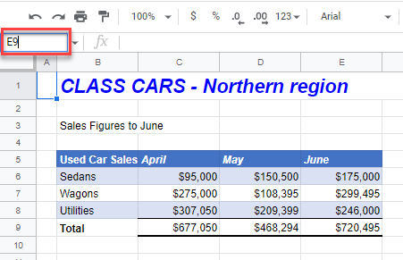
First of all, you have to enter any number of data in the Excel Sheet. Let’ take an example of data as given in the image below.

The example contains numbers in column B from cell B2 to B7. you have to now move this data to the cells of column D. Follow the next steps after entering the data.
Step 2 Select Data with Hover Over the Corner and Hold Mouse Left Button
Select your entire data using your mouse. After that, you have to hover over the corner of the selected data. You can hover to any corner position to the left, right, top and bottom.
Now, hold your mouse left button when you get the pointer sign as  .
.

The above example showing the selected data. You can also find the pointer sign when you hover over the corner. Click the corner when you get the sign  in the mouse pointer. Now, Keep your mouse hold for the next step.
Step 3 Drag-n-drop to the Cell to Move Data in Excel
You have to now drag your mouse to the required column cell. Drop the data when you reach the required cell to move to. It drops the whole data you have selected to move to the other cells.

The above example showing the image which you get when you drag your mouse.
Step 4 Final Moved Data
This is the final output contains the moved data to the cell of column D. The data copied from cell D2 to D7.

You can also move any of your data after selection using your mouse. If you want to move your data using a keyboard, you have to use the step-by-step process given below.
Shift One Cell Data to Another Using Only Keyboard in Excel Sheet
This is the method of only using the keyboard to change your data position. It’s the simple cut and paste method to shift data to other column cells.
Step 1 Put Your Data in Cell of Excel Sheet
Here, you also have to enter your data first in any cell of the Excel. Perhaps, you want to move the data already exist in the Excel sheet.

It depends upon you for which data you use. You can use any data to shift to other column cells. The above example showing the same data you have used in the above section.
Step 2 Select the Data Data Using Keyboard
Now, select your chosen data which you have to shift to the other cell. Use your keyboard left and right arrow key to move to the required data. Combination of shift and the arrow keys can be used to select the entire data.

The above image showing the selected data to shift to the other column cells.
Step 3 Press ‘CTRL + X’ to Cut Data
You have to cut the selected cell to shift to the other column cell. For this, press the keyboard key ‘CTRL + X’ to cut the data in Excel Sheet.

The above image showing the screen which you will get after pressing ‘CTRL + X’. This showing you are using the above data to cut in Excel Sheet.
Step 4 Go to Cell to Paste Data
After you perform the above step, you have to go to the cell where you want to place data. Press keyboard arrow keys to visit the required place for data.

The above example showing that you want to shift data to column D and start from cell D2.
Step 5 Press ‘CTRL + V’ to Paste and Move Data
The final step is to press the keyboard shortcut key ‘CTRL + V’. This is the key to paste the cut data to any required place of Excel Sheet.

The above image showing the shifted data to column D.
Change Data from One Column to Another in Excel
In addition to above all, you can also change or move one column data to another column. You have to first choose the data which you want to move. After that, follow the step-by-step guide given below with screenshots.
Step 1 Mouse Hover Over the Column Containing the Data
You have to first take your mouse to the column name which contains the required data. The pointer of the mouse changes to a down arrow like shape as given in the image.

The above image showing the data and the mouse pointer showing down arrow.
Step 2 Click Column Name to Select Data
Click the column name whose data you have to move. It selects all the cell of the clicked column name.

The above image showing the selected column containing the data to move.
Step 3 Mouse Right Click and Select ‘Cut’ Option
Now, you have to click the mouse right button to get various menu options. In the menu options, you have to select the ‘Cut’ option given on the menu.

You will get a highlighting column selection as showing in the image below.

Step 4 Click Column Name Where You Want to Shift Data
Click the column name to which you want to move the data. You will get a down arrow pointer for the mouse when you take your mouse to the column name.

The above example showing the select column where you have to place the data.
Step 5 Finally, press ‘CTRL + V’ to Paste Data
The final step is to paste the data using the keyboard shortcut ‘CTRL + V’. The below example image showing the pasted data to the new column.

You May Also Like to Read
- Copy Data In Alternate Rows Selected In Excel
- Quickly Select All Cells Of A Column In Excel
- Autofill Dates, Months And Current Time In Excel Sheet
Reference
MS Office Excel Doc to Move Cell and Cell Content
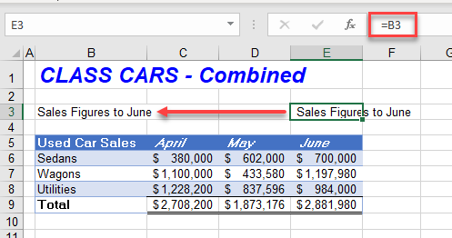
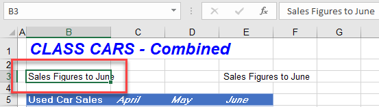
Moving on the sheet cells is carried out with the help of the cursor (controlled black rectangle). Most often, you need to move to the next cell when you fill in the Excel worksheets. But sometimes you need to move to any remote cells.
For example, you need to move to the end / start of the price list, etc. Each cell under the cursor is active. Viewing the contents of Excel worksheets can be divided into 2 types: first view by moving the cursor and the second view with the help of additional tools intended for viewing without moving the cursor. For example, the scroll bars of the sheet.
How to quickly move through cells in Excel with arrows keys is described in more detail below.
Moving the cursor to the next cell in the bottom
Move the cursor to the bottom (next) cell. When the program is loaded by default, the cursor is located on the cell with the address A1. You need to go to cell A2. There are 5 options for this solution:
- Just press the «Enter» key.
- Moving between the cells by using arrows keys. (All the arrows on the keyboard affect the movement of the cursor respectively with its direction).
- Point your mouse at the cell with address A2 and click the left mouse button.
- Use the «Go To» tool (CTRL+G or F5).
- Using the «Name» field (located to the left of the formula line).
Over time, in the process of working with Excel, you will notice that each option has its own advantages in certain situations. Sometimes it is better to click, and sometimes it’s better to move the cursor with the «Enter» key. Also, an additional example can serve this task and show how you can find solutions in several ways in Excel.
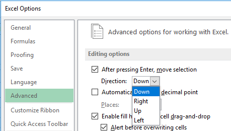
By default, the parameter for moving the cursor in Excel after pressing the «Enter» key is directed to the bottom, to the bottom cell (and if you press SHIFT+ENTER, the cursor will go to the top cell). If necessary, this can be changed in the program settings. Open the «Excel Options» window through the «FILE» — «Options» menu. In the opened window select the «Advanced» option. We are interested here with this option: «After pressing Enter, move selection Direction:». Below in the option specify the direction you want as shown in the picture:
Remember that the changes in this setting will make your work in Excel more comfortable. In certain situations of filling / changing data, you will often have to use this feature. It is very convenient when the cursor itself moves in the desired direction after entering data into the cell. And tables in sheets for data filling can be both vertical and horizontal.
Fast jump to selected remote cells
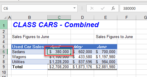
We moved along neighboring cells (C A1 to A2) in the above-described example. Try in the same way to move the cursor (black rectangle) to cell D3.
As you can see, in the given task the shortest way is to make 1 click with the mouse. After all, for the keyboard, it is 3 keystrokes.
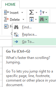
To solve this task, you can also use the «Go To» tool. To use it, you need to open the drop-down list of the «Find» tool on the «Home» tab and select the «Go To» option. Or you can press the combination of the hotkeys CTRL+G or F5.
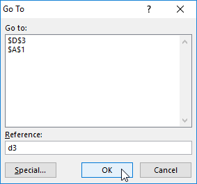
In the opened window enter D3 (you can enter it with small letters d3, and the program itself replaces small letters in large letters and in formulas it works in the same way), then click OK.
To quickly move the cursor to any address of a worksheet cell, it is also convenient to use the «NameBox» field which is in the upper left corner under the tool bar at the same level as the formula line. Enter in this field D3 (or d3) and press «Enter». The cursor will instantly move to the specified address.
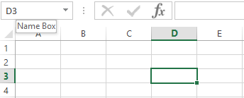
If the remote cell to which the cursor should be moved to make it active is situated in the same screen (view without scrolling), then it is better to use the mouse. If the cell needs to be searched but its address is known in advance, it is better to use the «NameBox» field or the «Go To» tool.
Most functions in Excel can be implemented in several ways. But in the further lessons, we will use only the shortest.
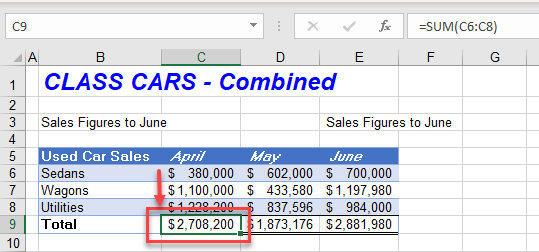
Move the cursor to the end of the worksheet
On a practical example, we quickly check the number of rows in a sheet.
Task 1. Open a new worksheet and place the cursor in any column. Press the END key on the keyboard, and then the «down arrow» (or use the combination of CTRL+»down arrow»). And you will see that the cursor has moved to the last line of the worksheet. If you press CTRL+HOME, the cursor moves to the first A1 cell.
Now check the address of the last column and number of columns.
To find out which column is the last in the worksheet, you must change the display style of the cells link addresses. To do this, go to «FILE» — «Options» — «Formulas» and tick the «R1C1 reference style» and then click OK.
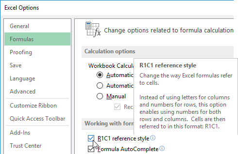
After that, the names of the columns will be replaced by numbers instead of letters. The sequence number of the last column of the sheet is 16384. After that, in the same order, uncheck the box to return the standard style of the columns with Latin letters.
The Excel ancestor was a program in the of a calculator-sheet style to help with work in the accounting department.
Therefore, the sheets resemble one large table. Now we have learned how to effectively navigate through the cells of this table, and then we will learn, how to effectively fill them with data.
There is no shortcut to success. Well.. there is when it comes to Excel.
If you want to be a lot more efficient in using Excel, I recommend you learn about some of the shortcuts and start using them as a part of your daily work.
You don’t need to know all the shortcuts (of course!), but it would be a big time saver to learn some to-do things you need to do daily/weekly.
Here is a list of 200+ Excel Keyboard Shortcuts that will save you tons of time.
Workbook Related Shortcuts
| What it Does? | Windows Shortcut | Mac Shortcut |
|---|---|---|
| Create a new blank Workbook | Ctrl + N | ⌘ + N |
| Displays the Open Dialog box to Open/Find a file | Ctrl + O | ⌘ + O |
| Saves the Workbook with its current file name, location, and file type | Ctrl + S | ⌘ + S |
| Opens the Save As dialog box | F12 | ⌘ + ⇧ + S |
| Opens the Print Preview Window | Ctrl + F2 | ⌘ + P |
| Maximize or Restore Selected Workbook Window | Ctrl + F10 | |
| Minimize Workbook | Ctrl + F9 | |
| Switch to the Next Workbook | Ctrl + Tab | |
| Switch to the Previous Workbook | Ctrl + Shift + Tab | |
| Close Current Workbook | ALT + F4 |
Excel Cell Editing Shortcut
| What it Does? | Windows Shortcut |
|---|---|
| Edit Active Cell | F2 |
| Start a New Line in the Same Cell | ALT + ENTER |
| Select One Character on the Right of the Cursor | SHIFT → |
| Select One Character on the Left of the Cursor | SHIFT ← |
| Jump one Word on the Right of the Cursor | Ctrl → |
| Jump one Word on the Left of the Cursor | Ctrl ← |
| Select one Word on the Right of the Cursor | Ctrl Shift → |
| Select one Word on the Left of the Cursor | Ctrl Shift ← |
| Delete One Character on the Left of the Cursor | Backspace |
| Delete One Character on the Right of the Cursor | Delete |
| Delete to the End of the line (from the cursor) | Ctrl + Delete |
| Cancel Entry | Esc |
Navigation Shortcuts in Excel
| What it Does? | Windows Shortcut |
|---|---|
| Move One Cell Up | ↑ |
| Move One Cell Down | ↓ |
| Move One Cell to the Right | → |
| Move One Cell to the Left | ← |
| Down One Screen | PageDown |
| Up One Screen | PageUp |
| Move One Screen to the Right | Alt + PageDown |
| Move One Screen to the Left | Alt + PageUp |
| Move to the Right Edge of the Data Region | Ctrl → |
| Move to the Left Edge of Data Region | Ctrl ← |
| Move to the Bottom edge of the data region | Ctrl ↓ |
| Move to the Top Edge of Data Region | Ctrl ↑ |
| Move to the Bottom-right used Cell in the Worksheet | Ctrl + End |
| Go to the First Cell in the Current Region | Ctrl + Home |
| Move to the Beginning of the Row | Home |
| Move to Next Worksheet | Ctrl + PageDown |
| Move to the Previous Worksheet | Ctrl + PageUp |
General Excel Shortcuts
| What it Does? | Windows Shortcut |
|---|---|
| Opens Help | F1 |
| Repeats the last command or action | Ctrl + Y |
| Repeats the Last Action | F4 |
| Undo | Ctrl + Z |
| Spell Check | F7 |
| Apply Data Filter | Ctrl + Shift + L |
| Activate Filter (when the cell with filter is selected) | Alt + ↓ |
| Display Go To Dialog Box | F5 |
| Display Go To Dialog Box | Ctrl + G |
| Recalculate All Workbooks | F9 |
| Calculate Active Worksheet | Shift + F9 |
| Display the Print Menu | Ctrl + P |
| Turn On End Mode | End |
Cut, Copy, and Paste Shortcuts in Excel
| What it Does? | Windows Shortcut |
|---|---|
| Copy Selected Cells | Ctrl + C |
| Cut Selected Cells | Ctrl + X |
| Paste Content from the Clipboard | Ctrl + V |
| Copy Formula from the Cell Above | Ctrl + ‘ |
| Copy Value from the Cell Above | Ctrl + SHIFT + ‘ |
| Display Paste Special Dialog Box | Ctrl + Alt + V |
Data Entry Shortcuts in Excel
| What it Does? | Windows Shortcut |
|---|---|
| Enter and Move Down | Enter |
| Enter and Remain on the Same Cell | Control + Enter |
| Enter and Move Up | Shift + Enter |
| Enter and Move right | Tab |
| Enter and Move Left | Shift + Tab |
| Enter Same Data in All Selected Cells | Control + Enter |
| Display AutoComplete list | Alt + ↓ |
| Fill Down | Ctrl + D |
| Fill Right | Ctrl + R |
| Insert Current Date | Ctrl + ; |
| Insert Current Time | Ctrl + Shift + ; |
| Start a New Line in the Same Cell | Alt + Enter |
| Cancel Cell Entry | ESC |
Clear Shortcuts in Excel
| What it Does? | Windows Shortcut |
|---|---|
| Clear Everything | Alt + H + E + A |
| Clear Formats Only | Alt + H + E + F |
| Clear Content Only | Alt + H + E + C |
| Clear Hyperlinks Only | Alt + H + E + L |
| Clear Comments Only | Alt + H + E + M |
Selection Shortcuts in Excel
| What it Does? | Windows Shortcut |
|---|---|
| Select the Current Region / Select All | Ctrl + A |
| Select Visible Cells in the Current Region | Alt + ; |
| Select the Current Region Around the Active Cell | Ctrl + Shift + * |
| Select Entire Row | Shift + Space |
| Select Entire Column | Ctrl + Space |
| Select All Cells that Contain Comments | Ctrl + Shift + O |
| Select Row Differences | Ctrl + |
| Select Column Differences | Ctrl + Shift + | |
| Select Direct Precedents | Ctrl + [ |
| Select all Precedents | Ctrl + Shift + { |
| Select Direct Dependents | Ctrl + ] |
| Select all Dependents | Ctrl + Shift + } |
Extending the Selection Shortcuts
| What it Does? | Windows Shortcut |
|---|---|
| Extend Selection to the Right by One Cell | Shift + → |
| Extend Selection to the Left by One Cell | Shift + ← |
| Extend Selection Upwards by One Cell | Shift + ↑ |
| Extend Selection Downwards by One Cell | Shift + ↓ |
| Extend the Selection to the Right till the Last Cell | Ctrl + Shift + → |
| Extend the Selection to the Left till the Last Cell | Ctrl + Shift + ← |
| Extend the Selection Upwards to the Last Cell | Ctrl + Shift + ↑ |
| Extend Selection Upwards by One Screen | Shift + PageUp |
| Extend Selection Downwards by One Screen | Shift + PageDown |
| Extend Selection to the Right by One Screen | ALT + Shift + PageUp |
| Extend Selection to the Left by One Screen | ALT + Shift + PageDown |
| Extend Selection to the Start of the Row | Shift + Home |
| Extend Selection to First Cell in the Worksheet | Ctrl + Shift + Home |
| Extend Selection to the Last Cell in the Worksheet | Ctrl + Shift + End |
| Toggle Extend Selection Mode | F8 |
Alignment Shortcuts
| What it Does? | Windows Shortcut |
|---|---|
| Align Content to the Center of the Cell | Alt + H + A + C |
| Align Content to the Left of the Cell | Alt + H + A + L |
| Align Content to the Right of the Cell | Alt + H + A + R |
| Align Content to the Middle of the Cell | Alt + H + A + M |
Hide/Unhide (Rows, Columns, Objects) Shortcuts
| What it Does? | Windows Shortcut |
|---|---|
| Hide Selected Rows | Ctrl + 9 |
| Hide Selected Columns | Ctrl + 0 |
| Unhide Hidden Rows in Selection | Ctrl + Shift + 9 |
| Unhide Hidden Columns in Selection | Ctrl + Shift + 0 |
| Show/Hide Objects | Ctrl + 6 |
Insert Shortcuts
| What it Does? | Windows Shortcut |
|---|---|
| Insert New Line in the Same Cell | Alt + Enter |
| Insert New Worksheet | Shift + F11 |
| Insert Row/Cell (shows a dialog box) | Ctrl + Shift + = |
| Insert Current Date | Ctrl + ; |
| Insert Current Time | Ctrl + Shift + ; |
| Insert Table | Ctrl + T |
| Insert Hyperlink | Ctrl + K |
| Insert Argument Names into Formula | Ctrl + Shift + A |
| Insert/Edit Cell Comment | Shift + F2 |
| Delete Row/Cell (shows the dialog box) | Ctrl – |
Formatting Shortcuts in Excel
| What it Does? | Windows Shortcut |
|---|---|
| Make Text Bold | Ctrl + B |
| Make Text Italics | Ctrl + I |
| Place outline Border around the Selected Cells | Ctrl + Shift + 7 |
| Remove Outline Border | Ctrl + Shift + _ |
| Underline Text | Ctrl + U |
| Apply Strikethrough Format | Ctrl + 5 |
| Apply Indent | Alt H 6 |
| Remove Indent | Alt H 5 |
| Increase Font Size by One Step | Alt H F G |
| Decrease Font Size by One Step | Alt H F K |
| Apply the Number format with Two Decimal Places, Thousands Separator, and a Minus Sign for Negative Values | Ctrl + Shift + ! |
| Apply the Date format with the Day, Month, and Year | Ctrl + Shift + # |
| Apply the Currency Format with Two Decimal Places | Ctrl + Shift + $ |
| Apply the Percentage Format with No Decimal Places | Ctrl + Shift + % |
| Apply the Time format with the Hour and Minute, and indicate AM or PM | Ctrl + Shift + @ |
| Apply the General Number Format | Ctrl + Shift + ~ |
| Apply the Exponential Format | Ctrl + Shift + ^ |
| Displays the Format Style Dialog Box | Alt + ‘ |
| Displays the Format Cells Dialog Box | Ctrl + 1 |
| Displays the Font Dialog Box | Shift + Ctrl + F |
Excel Formula-Related Shortcuts
| What it Does? | Windows Shortcut |
|---|---|
| Insert Autosum Formula | Alt + = |
| While Typing a Formula, Switches Cell Reference from Absolute to Relative | F4 |
| Expand/Collapse Formula Bar | Ctrl + Shift + U |
| Display the Insert Function Dialog Box | Shift + F3 |
| Enter a Formula as an Array Formula | Ctrl + Shift + Enter |
| Evaluate Part of the Formula | F9 |
| Select the Array Containing the Active Cell | CTRL + / |
| Select All Cells Directly or Indirectly Referenced by Formulas in the Selection | CTRL + [ |
| Select Cells that Contain Formulas that Directly or Indirectly Reference the Active Cell | CTRL + ] |
| Toggle Value/Formula display | Ctrl + ` |
| Rechecks dependent formulas and then calculates all cells in all the open workbooks | Ctrl + Alt + Shift + F9 |
Find and Replace Shortcuts
| What it Does? | Windows Shortcut |
|---|---|
| Display Find and Replace Dialog Box (Find Selected) | Ctrl + F |
| Display Find and Replace Dialog Box (Replace Selected) | Ctrl + H |
| Find Next Match | Shift + F4 |
| Find the Previous Match | Ctrl + Shift + F4 |
Conditional Formatting Shortcuts
| What it Does? | Windows Shortcut |
|---|---|
| Open Conditional Formatting Dialog Box | Alt O D |
| Clear Conditional from Selected Cells | Alt H L C S |
| Clear Conditional from the Entire Worksheet | Alt H L C E |
Charting Shortcuts
| What it Does? | Windows Shortcut |
|---|---|
| Inserts Chart in the Worksheet (using the selected data) | Alt + F1 |
| Inserts a ChartSheet with a Chart (using the selected data) | F11 |
Drag (Mouse) Shortcuts
| What it Does? | Windows Shortcut |
|---|---|
| Drag and Copy the selected cells | Ctrl + Drag |
| Drag and Cut the selected cells | Drag |
| Duplicate Worksheet | Ctrl + Drag |
| Switch Position of Cells/Rows/Columns | Shift + Drag |
Named Ranges Shortcuts
| What it Does? | Windows Shortcut |
|---|---|
| Get a List of All Defined Named Ranges | F3 |
| Create Named Range from Selection | Ctrl + Shift + F3 |
| Define Name Dialog Box | Ctrl + F3 |
Pivot Table Shortcuts
| What it Does? | Windows Shortcut |
|---|---|
| Display Insert Pivot Table Dialog Box | Alt + N + V |
| Open Pivot Table Wizard | Alt + D + P |
| Select Entire Pivot Table (excluding Report Filters) | Ctrl + A |
| Add/Remove Checkmark for Selected Field in PivotTable Field List | Space |
| Group Selected Pivot Table Items | Alt + Shift + → |
| UnGroup Pivot Table Items | Alt + Shift + ← |
| Select the Next Item in PivotTable Field List or Items List | ↓ |
| Select a Previous Item in PivotTable Field List or Items List | ↑ |
| Select Last Visible Item in List | End |
| Select First Visible Item in List | Home |
| Open Field List for Active Cell | Alt + ↓ |
| Hide Selected Item or Field | Ctrl + – |
| Opens Calculated Field dialog box (when the data field is selected) | Shift + Ctrl + = |
| Opens Calculated Item Dialog box (when field heading cell is Selected) | Shift + Ctrl + = |
Others Shortcuts
| What it Does? | Windows Shortcut |
|---|---|
| Restore Window Size | Ctrl + F5 |
| Move Window | Ctrl + F7 |
| Resize Window | Ctrl + F8 |
| Previous Window | Ctrl + Shift + F6 |
| Next Pane | F6 |
| Previous Pane | F8 |
| Extend Mode | Shift + F10 |
| Display Shortcut Menu | Shift + F6 |
| Turns On the Add to Selection Mode | Shift + F8 |
VBA Shortcuts
| What it Does? | Windows Shortcut |
|---|---|
| Opes the VBA Editor and also switches between Excel Worksheet and the VBA editor | Alt + F11 |
| Open VB Help | F1 |
| View Object Browser | F2 |
| View Properties | F4 |
| View Code window | F7 |
| View Immediate window | Ctrl + G |
| View Shortcut Menu | Shift + F10 |
| Run a Sub/UserForm | F5 |
| Step Into the code | F8 |
| Step Over | Shift + F8 |
| Step Out | Ctrl + Shift + F8 |
| Run to Cursor | Ctrl + F8 |
| Toggle Breakpoint | F9 |
| Clear All Breakpoints | Ctrl + F9 |
| Close VBA Editor and Return to the Excel Worksheet | Alt + Q |
Useful Excel Resources:
- 20 Excel Keyboard Shortcuts that Will Impress Your Boss.
- 100+ Excel Interview Questions + Answers.
- Excel Functions (Videos + Examples).
- Free Excel Templates.
- Free Online Excel Training.
- 20 Advanced Excel Functions and Formulas (for Excel Pros)
- 10 Excel Pivot Table Keyboard Shortcuts
There are two ways to press the shortcut keys depending on the separator character used in the sequence.
+ Plus
The + (plus) between keys means press & hold the keys together in order. For example, to press the shortcut Ctrl+Shift+L to Toggle Filters, you will:
Press & hold Ctrl, then press & hold Shift, then press L. Then release all keys.
, Comma
The , (comma) between keys means press & release each key in order. For example, to press the shortcut Alt,E,S to open Paste Special, you will:
Press & release Alt, then press & release E, then press & release S.
Laptop Keyboards
If you are using a laptop keyboard then you might be limited on the some of the shortcuts you can press. Laptop keyboards tend to have smaller keyboards and don’t always contain keys like Page Up, Page Down, Menu, etc.
You might also need to press the Fn (function) key in combination with the function keys F1 to F12. Some laptops have Fn Lock Mode so that you don’t have to press Fn with the the function keys.
Checkout our post on the Best Keyboards for Excel Keyboard Shortcuts to learn more.
Below is a listing of most major shortcut keys and key combinations usable in Microsoft Excel. See the computer shortcuts page if you are looking for shortcut keys used in other programs.