
You may be familiar with Microsoft Excel. This application made by Microsoft Corporation is the application with the most users in the world in 140+ countries. This application has a myriad of Excel formulas that can accurately present numbers and data.
The primary function of Microsoft Excel is calculation, which is why it has been used by many users, both students and office workers. Despite other spreadsheet programs (competitors), Excel maintained its dominance and even became an industry standard.
Apparently, Excel seems too good to be true. All you have to do is enter an Excel formula, and almost everything you need to do manually can be done automatically. Use the best accounting software to do the cash flow forecast appropriately and analyze financial statements more optimally.
If you need to combine two sheets with the same data, Excel can do this. Do you need help with mathematics? Excel can do this. Are you using data from multiple cells? Excel can do this too.
In this article, you will understand the function of Excel in different professional fields. Then you’ll understand what formulas you need to know. Later, you will be able to apply automatic calculations to be used according to your needs.
Table Of Content
- The Uses of Excel in Professional Fields
- Complete Excel Formulas with Their Functions
- Conclusion
Also Read: 5 Common Bookkeeping Mistakes on Small Businesses
The Uses of Excel in Professional Fields
Many job openings require candidates to master Excel. Not surprisingly, excel is needed by a wide variety of fields of work that require data collection.
To that end, we will present the following professions, which can benefit from the use of Excel, among others:
Accountancy
It is widespread for accountants to be able to use Excel. The field of accounting benefits from using Microsoft Excel in several ways, including making it easier to calculate corporate profit and loss, identify large profits over a period, calculate employee salaries, and more.
An accountant can facilitate his work by using the accounting system as a tool he worked. The system can provide convenience in managing the company’s financial circulation and calculating it optimally and accurately.
Also Read: Salary Slip: Understanding, Benefits, Format, Example
Mathematical calculations
The next advantage of using Microsoft Excel is mathematical calculations. Use calculations to find data from numbers, subtractions, multiplications, and divisions, as well as various other variations such as calculating the slope.
Data processing
In data management, there are helpful excel formulas, including managing statistical databases, calculating data, searching for median values, and averages, and searching for the maximum and minimum values of data sets.
Graphic creation
Excel allows you to create graphics. Such as graphing population development data for one year, the graph of student library visits for one year, the student graduation graph for six years, the graph of student number development for three years, and others.
Table operations
The last application is to be able to operate the table. With a total of 1,084,576 rows and 16,384 columns in Microsoft Excel, it will make it easier for you to enter data that requires a large number of columns and rows.
Complete Excel Formulas with Their Functions
In addition to the functionality and use of Microsoft Excel mentioned earlier, operating this Excel program requires Excel formulas. Each formula has a different function that you can use for a specific need.
Here are the Excel formulas you need to know, among others:
| Formulas | Functional Description |
| SUM | Summing |
| AVERAGE | Looking for Average Values |
| AND | Finding Value by comparison and |
| NOT | Finding Value with Exceptions |
| OR | Finding Value by Comparison or |
| SINGLE IF | Looking for Values If Conditions ARE RIGHT/WRONG |
| MULTI IF | Finding Values If Conditions ARE RIGHT/WRONG With Many Comparisons |
| AREAS | View The Number of Areas (Range or Cells) |
| CHOOSE | View Selection Results Based on Index Numbers |
| HLOOKUP | Search for Data from a table organized in a horizontal format |
| VLOOKUP | Search for Data from a table arranged in an upright format |
| MATCH | Displays the position of a specific cell address |
| COUNTIF | Counting the Number of Cells in a Range with specific criteria |
| COUNTA | Counting the Number of Filled Cells |
| CEILING | Round the number up |
| FLOOR | Rounds numbers down |
| DAY | Looking for The Value of the Day |
| MONTH | Searching for the Value of the Moon |
| YEAR | Looking for Year Value |
| DATE | Get a Date Value |
| LOWER | Change text letters to lowercase |
| UPPER | Change Text Letters to UpperCase |
| PROPER | Change the Initial Character of the Text To UpperCase |
For more information about how to use the excel function formulas mentioned above, here is a detailed description, along with examples:
SUM
This Excel summation formula has the primary function of summing numbers in specific cells. However, it is also often used to complete a job or task quickly.
To use SUM, first create a summation table and enter the summation formula below. For example, =SUM(G8:H8), or as shown in the image below:
Then, if the SUM formula has been entered, press enters to specify the amount. As shown in the picture below:
AVERAGE
The primary function of the AVERAGE formula or the average formula in Excel is to find the average value of a variable. The trick is to create a table for grades and then enter the AVERAGE formula to determine the student’s grade point average. For example, =AVERAGE(D2:F2), as in the following image:
If you enter the AVERAGE formula, press enters to see the result, shown in the image below.
AND
The AND formula function generates a TRUE value if all previously tested arguments are correct or can return a FALSE value if all arguments or answers are incorrect.
To determine TRUE or FALSE, you must create a table and enter THE FORMULA AND. For example, =AND(G7>I7).
This technique is usually used to help fill out questionnaires or answer question columns to speed up the value-setting process.
NOT
The NOT formula has the opposite function of the AND formula because it produces TRUE if the condition tested is FALSE and FALSE if the condition tested is TRUE.
The first step is to create a table and enter the FORMULA NOT to find out the results. For example, as shown in the diagram below, =NOT(G7>J7).
OR
The OR is the following excel formula that will produce TRUE data if some given argument is correct. If all of the arguments presented are incorrect, the answer is FALSE.
A student’s average test score result is an example of how OR can use it in Excel. If it is less than 70, he must repeat the course; if it is greater than 70, the student graduates.
SINGLE IF
The IF function is to return a value that, when examined, is TRUE and another value that is visible as FALSE.
Not much different from the technique of using formulas in OR. It just seems more straightforward.
For example, when a student’s average grade is less than 75, that student does not graduate, and vice versa. How to create an IF formula is =IF(J8<75;” NOT GRADUATING”;” PASS”). To be clear, take a look at the following image:
After entering the formula, press enters, and the result will match what you ordered.
MULTI IF
This formula is a further lesson from SINGLE IF, but if SINGLE IF only uses only one condition with two options, The MULTI IF uses two terms and three options.
A Double/Multi FORMULA is a type of logic-IF formula consisting of 2 or more IF in formula writing. If a single IF only needs 1 IF, for example, =IF(B2=>=70;” Graduated”;” Failed”) then Double IF requires more than 1 IF, for example, =IF(B2>=70;” Good”;IF(B2>=50;” Enough”;” Less”)).
So that the full Excel formula will provide Syntax on Double / Multi IF, among others:
=IF(Logical_Test; Value_If_True;IF(Logical_Test; Value_If_True; Value_If_False))
AREAS
You can use the usability of AREAS if you want to calculate the number of areas you want to select. The AREAS formula can use the formula =AREAS(G6:K8).
The result is one area. The results are based on the example in the image of selecting only one range of cells.
CHOOSE
The primary function of a CHOOSE formula is to display selection results based on index numbers or sequences in reference (VALUE) that contain text, numeric, formula, or range names. The image below shows an example of how to write the CHOOSE formula.
Meanwhile, the results of the CHOOSE formula are shown in the image below.
HLOOKUP
The HLOOKUP function displays data from tables arranged horizontally. However, The arrangement of tables or data in the first row should be based on small to large sequences or raising them.
For example, the number 1,2,3,4… Or the letter A-Z. Sort by ascending the menu if you previously typed randomly. Cases like the ones listed below are examples.
=HLOOKUP(Cells that contain packet types; Range cell table details costs; The location of the data column you want to retrieve;0).
VLOOKUP
The primary function of the VLOOKUP formula is almost identical to the HLOOKUP formula; The difference is that the VLOOKUP formula displays data from tables arranged in an upright or vertical format. The requirement is that the first row of the data table is prepared in small to large order or up.
For example 1,2,3,4… Or the letter A-Z. For example 1,2,3,4… Or the letter A-Z. Sort through the Ascending menu if you previously typed randomly.
MATCH
The MATCH function is one of the components of an Excel formula that you can use to perform lookups or reference data searches.
The MATCH function works by finding the relative position of a value in a range or array and generating a number that is the index of the cell’s relative position that contains the value it is looking for.
The use of the Excel MATCH function must follow the syntax rules, namely MATCH(lookup_value, lookup_array, [match_type])
To better understand, understand the image below:
COUNTIF
COUNTIF is a helpful formula for counting the number of cells that have the same criteria. As a result, you no longer have to struggle with data sorting.
Assume you’re doing a survey. You want to know how many civil servants there are out of 20 respondents. As a result, you can use the following formulas:
To get started, all you need to do is enter the range of cells you want to identify into the COUNTIF formula (B2:B21)
Then, enter the cell calculation criteria, namely “PNS” (must be in quotation marks).
This formula produces a result of 7. So, out of 20 respondents, seven were civil servants.
COUNTA
COUNTA has the function of counting the number of cells that contain numbers and the number of cells that contain anything. As a result, you can determine the number of cells that are not empty.
Assume that cells A1 through D1 are words and cells G1 through I1 number. Therefore the use of the formula is =COUNTA(A1:I1)
That results in 7 because the empty cells are only E1 and F1.
CEILING
The CEILING formula can round the number UP at the multiple values of a specific number. The formula is CEILING (CELLS number; Multiples).
Misalnya, CEILING(G9;100). Then the number on Cells G9 will be rounded up with a multiple of 100.
FLOOR
If the previous use of the formula is to round to the nearest integer and above, the FLOOR formula is used to round to the nearest integer. The formula is almost identical to the one for CEILING, but with the addition of FLOOR.
The FLOOR formula is FLOOR (Number cell; Multiples).
DAY
The DAY formula is used to find the date type data’s day (in the numbers 1-31). Consider the DAY function (column B). The date data in column A will be extracted and converted into numbers 1-31, following the explanation through the image:
After entering the formula =DAY(NUMBER), press enters and see the results below:
MONTH
Almost similar to the DAY formula, the use of the MONTH formula to search for months (in numbers 1-12) from date type data. For example, the use of the MONTH function (column K) of a column I date data, after extracting it, produces the numbers 1-12 as in the figure below:
YEAR
Meanwhile, there is a YEAR formula. The way you use this formula is similar to the way the previous two formulas were. The use of the YEAR formula takes years (in the range of 1900-9999) from date-type data.
DATE
The DATE formula has a function that allows you to get date data types by entering years, months, and days. The DATE function is the opposite of the DAY, MONTH, and YEAR functions, which describe month and year-type data from their respective dates.
Year, month, and day data in the form of numbers combined with the DATE function generate data with data types, as shown in the figure below. Date formula writing image, namely:
LOWER
The lower formula function converts all uppercase letters in the text to lowercase. To use the formula, type the LOWER command, and texts will convert the desired writing to lowercase.
For example, when implementing the LOWER formula with the formula =LOWER (Don’t Forget to Use HashMicro Software), the result is “don’t forget to use has micro software.”
UPPER
In addition to lower formulas, Microsoft Excel includes upper formulas. The use of UPPER is to convert all text containing lowercase letters into uppercase, the opposite of the LOWER function.
For example, if you type UPPER (hashmicro), your writing will be entirely in capital letters.
PROPER
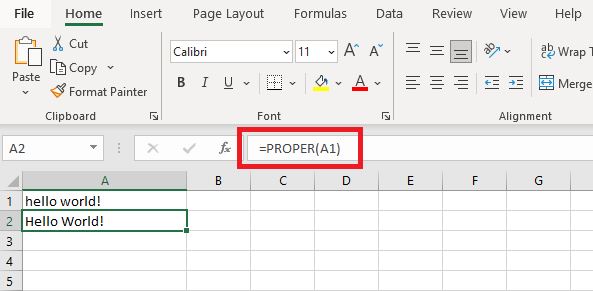
Sometimes you forget to write sentences in all lowercase letters and no capital letters. So with the PROPER formula, you can capitalize on the first character in each word while keeping the rest. The formula is APPROPRIATE (text).
Conclusion
Although understanding Excel entirely takes time, you will be familiar with all the correct formulas and applications.
In a company, the use of Excel is overwhelming, especially in presenting data, statistics, and company finances such as salaries. The digital world is bringing corporate transformation to provide information and payroll more easily with automated systems. You can use HashMicro accounting software as a tool to calculate financial circulation optimally and accurately.
Moreover, HashMicro has a system that helps with all your human resource and employee administration tasks. With HashMicro’s HRM Software, calculates salaries, and manages leave and attendance lists, reimbursement processes, timesheets, and other operational activities in just seconds.
Produce reports accurately and comprehensively like thousands of large companies that have joined HashMicro. To check out more, click here.
MS Excel is one of the most popular data analysis tools in the world. More and more companies greatly depend on this software and quite a lot of people are using it on a daily basis. However, from my experience, not many are taking full advantage of the opportunities that the program can offer. Here is my list of the top 20 most important and useful Excel functions, which everyone should use in order to increase his efficiency. Excel functions are also highly recommended over manual calculations, as they can greatly reduce the number of errors. Last but not least, learning these formulas is a wonderful opportunity for you to improve your Excel knowledge and become a confident MS Excel user.
Table of Contents
1. Sum
“Sum” is probably the easiest and the most important Excel function at the same time. You can use it to calculate sum of a range of cells.
= SUM(A1:A10) or = SUM(A1,A10)
In this example, the first formula sums the cells from A1 to A10. The second sums only cells A1 and A10. You can play around with it and try to use different ranges in order to get used to it. Please note that you can also use specific values inside the function, instead of references.
2. Average
Another very important function. As the name suggests, this formula estimates the average number from a range of cells. Suppose that we have a range of values in column A.
= AVERAGE(A1:A10)
This will return the average value of the cells from A1 to A10.
3. If
Another must-use formula. It is relatively easy to use and very powerful at the same time. You can use this function to check whether a statement is true or false and return the stated value.
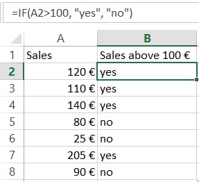
= IF(A2>100,"yes","no")
Here, the formula looks for sales over 100 € in cell “A2”. If this statement is true, the formula returns “yes”. If the sales are below 100 €, the formula returns “no”.
4. Sumif
Sumif is another very useful Excel formula. The formula will sum values, if a certain condition is met.
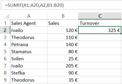
= SUMIF(A1:A20,A2,B1:B20)
Let’s have a look at the above example. We have sales agents who register a certain number of sales. We want to know the total number of sales for each agent. The function = SUMIF (A1: A20, A2, B1: B20) sums the values of cells B1: B20 that correspond to the text in cell A2 (in the case of Ivailo). The guy has registered a total sales of 325 €. We can use the formula to calculate the turnover of the other agents as well.
5. Countif
Countif is a very useful function that works like a sumif. It sums under a certain condition. The difference between sum and count is that the count function counts the number of cells where certain condition is true. On the contrary, the sumif function sums the values inside the cells.
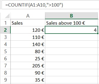
= COUNTIF(A1:A10,">100")
The formula in the above example checks how many times sales are made over 100 € and returns the number of occurances. You can also include more than one criteria by using countifs for that purpose.
PS: If you are not sure about the syntax of a function, you can always use the Insert function option in Excel (Just press the function sign on the left side of the function bar). In the next example, we will demonstrate how this works.
6. Counta
This formula counts the number of cells from a specific range which are not empty. It is very useful when you have thousands of rows and you want to know where this all ends.
Example 6.
= COUNTA(A:A)
This will give you the number of rows that contain value, text or any other symbol.
7. Vlookup
Probably the most powerful Excel function. Very useful when you have to deal with more than one table, different sheets or even a different workbook. Vlookup lets you exract data from one table to another.
Let’s continue with the above example by adding another column “A” with customer numbers.
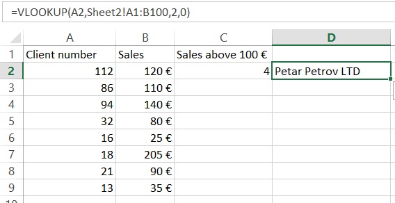
Note that there is information about the sales and the customer numbers, but the customers’ names are missing. However, we have another Excel sheet (Sheet2) with client names and client numbers.
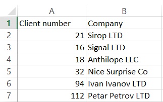
Instead of taking our time to look from Sheet1 to Sheet2 and search for a match manually for each single row, we should use the following formula:
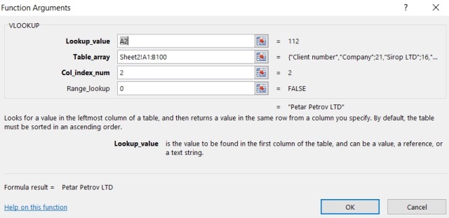
= VLOOKUP(A2,Sheet2!$A$1:$B$100,2,0)
This formula looks up for the value in cell A2 (112 in our case) in sheet2, columns A & B (the “$” signs mean that we want to have a constant lookup range). The function then returns the value from the second column. The last part of the formula is 0. In this way we tell Excel to look for a match in a shuffle order, not only in one row.
Now, try to construct your own vlookup formula using the insert formula option.
In our case, it looks like this:
8. Left, Right, Mid
The left, right and mid functions are very important functions that allow you to extract a definite number of symbols from a string
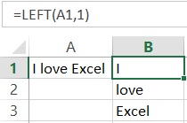
= Left(A1,1) or = MID(A1,4,6) or = RIGHT(A1,5)
In our example, with the Left formula, we take the first character from the left side. With the right formula we can do the same, but with the symbols from right to left. Keep in mind that the space is also a symbol.
9. Trim
Another exceptional MS Excel feature. The trim function removes unnecessary spaces after the words, when they are more than one. This can happen quite often in Excel. It may be that the information is extracted from different databases and it is full of unnecessary empty spaces between the words. This can be a huge problem because your Excel fomulas may not work. To get rid of the annoying empty spaces, we use the Trim formula.
= TRIM(A1)
In this example, the formula will remove any extra spaces in case it finds more than one.
10. Concatenate
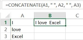
This is a handy Excel function that comes to help when we want to combine cells.
Here, we want to merge cells A1, A2, and A3. This can be done with the following function:
= CONCATENATE(A1,A2,A3)
In this way, however, we will not have any spaces between the words. To add blanks between “I” and “ love”, we need to add a space. This can be addressed by adding quotes inside the function:
= CONCATENATE(A1," ",A2," ",A3)
PS: You can also merge the cells by simply adding:
= A1&" "&A2&" "&A3
Try it yourself!
11. Len
Another amazing formula that can be applied in many situations. It is widely used for construction of more complicated formulas.
= LEN(A1)
This function will count the number of symbols in a cell.
12. Max
The max function returns the largest value from a range.
= MAX(A2:A8)
This formula will look in cells A2:A8 and it will then extract the highest value from this range.
13. Min
The min function functions in a similar way as the max function, however it gives the opposite result. It extracts the lowest value from a range of data.
= MIN(A2:A8)
The formula from the above example will return the smallest number from the selected cells in column “A”.
14. Days
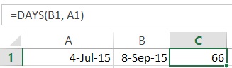
This is the function when you need to estimate the number of days between two days in a spreadsheet.
= DAYS(B1,A1)
The formula will return the number of days that have passed.
15. Networkdays
Sometimes you want to work with working days only. This function operates in a very similar way to the above example. The difference is that it returns the working days that have passed, excluding the weekends.
16. SQRT
This is pretty simple and quite useful at the same time. As the name suggests, the formula gives the square root of a number
= SQRT(1444)
This will return the square root of 1444 (38). You can also use cell reference here, just like in many other Excel formulas.
17. Now
Sometimes you need to know the current date, when you open Excel spreadsheet.
Example
= NOW()
This will return the current date. Do not forget to set the format to date. You can play around with it as much as you want. You can, for example, add or subtract days. =Now() -14 will return the date before two weeks.
18. Round
The Round function is very useful, when you have to work with rounded numbers. Excel can show numbers to a specific character, but retains the original number and uses it for calculations. In some cases, however, this could be an issue and we need to work with rounded numbers only. In such cases, the ROUND function comes into our help.
= ROUND(B1,2)
In the example, the number is rounded to the second decimal.
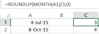
19.Roundup
This is a variation of the round formula that can help a lot In some cases. It rounds the value up to the closest integer. It is very useful in combination with other Excel formulas.
Let’s have a look at this example:
= ROUNDUP(MONTH(B3)/3,0)
Here, we want to find in which quarter of the year a current date is. The secret to this formula is simple math. The function takes the number of the month, e.g January is 1, February is 2, etc. and then divides it by 3, rounding up to the closest higher number.
20. Rounddown
Rounddown works in a similar way as Roundup, however it rounds the number down to the closest integer
= ROUNDDOWN(20.65,0)
This will return 20.
Excel has many useful functionalities. This article attempts to present the most important formulas in MS Excel in the best comprehensive way possible. We believe that these functions are a very good base for those of you who want to develop their Excel skills. By mastering these formulas, you can easily handle most day-to-day situations that may occur when working with Excel and it is a really nice opportunity further develop your skills.
© 2017 Atanas Yonkov
Read more: 18 ready-to-use VBA Codes that will save your day
Literature:
1. ExcelChamps.com: The Top 15 Excel Functions you NEED to know — Excel by Joe.
3. BG Excel.info: Top 11 most popular Excel functions.
The functions you need, and use the most!
Guest Post with minor edits by Ben Currier

Before we start
When working with Excel it’s important to remember that :
– Cells are referenced by their coordinates, e.g. A1 is the cell in the first column and first row.
– Formulas begin with an equal sign (=).
– You can use absolute references (e.g. $A$1) or relative references (e.g. A1) in formulas. Absolute references don’t change when you copy a formula, while relative references will adjust based on the new location.
– You can use the tab key to move between cells.
Now, let’s take a look at the top eleven most-used formulas in Excel:
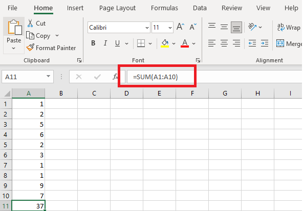
1 – SUM()
SUM: This is probably Excel’s most basic and commonly used formula. It simply adds up the numbers within a range of cells. For example, if you wanted to sum up cells A1 to A10, you would use the formula =SUM(A1:A10).
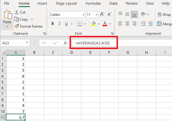
2 – AVERAGE()
AVERAGE: As the name suggests, this formula returns the average of a range of cells. So, if you had cells A1 to A10 containing numbers, you could find the average with the formula =AVERAGE(A1:A10).
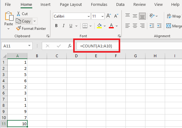
3 – COUNT()
COUNT: This formula counts the number of cells in a range that contains numbers. So, if you wanted to count how many cells in a range contained numbers, you could use the formula =COUNT(A1:A10).
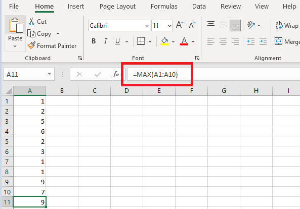
4 – MAX()
MAX: This formula returns the largest value in a range of cells. So, if you had cells A1 to A10 containing numbers, you could find the largest number with the formula =MAX(A1:A10).
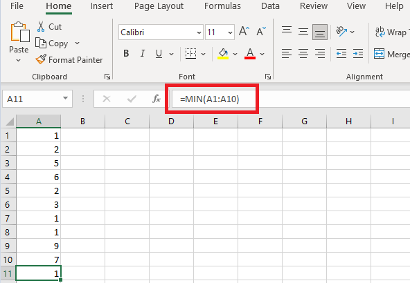
5 – MIN()
MIN: This formula returns the smallest value in a range of cells. So, if you had cells A1 to A10 containing numbers, you could find the smallest number with the formula =MIN(A1:A10).
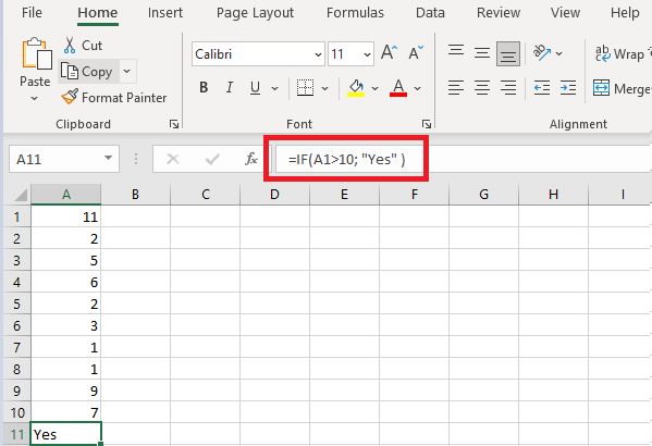
6 – IF()
IF: This is a very powerful and commonly used formula. It basically allows you to test a condition, and then return one value if the condition is met, and another value if it isn’t. For example, you could use the formula =IF(A1>10, “Yes”) to test if the value in cell A1 is greater than 10. If it is, the formula will return the word “Yes”, if not, it will return the word “No”.
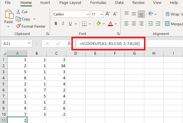
7 – VLOOKUP()
VLOOKUP: This is another very powerful and commonly used formula. It allows you to look up a value in one table, and then return a corresponding value from another table. For example, you could use the formula =VLOOKUP(A1; B1:C10; 2; FALSE) to look up the value in cell A1 in the table defined by cells B1 to C10. If a match is found, the formula will return the value in column 2 of the table (i.e., the value in cell C1 if A1 contains the value in B1).
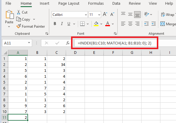
8 – INDEX() & MATCH()
INDEX/MATCH: This is a similar formula to VLOOKUP, but it is often considered to be more powerful and flexible. It also allows you to look up a value in one table, and then return a corresponding value from another table. For example, you could use the formula =INDEX(B1:C10, MATCH(A1, B1:B10, 0), 2) to look up the value in cell A1 in the table defined by cells B1 to C10. If a match is found, the formula will return the value in column 2 of the table (i.e., the value in cell C1 if A1 contains the value in B1).
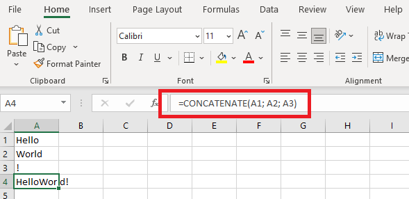
9 – CONCATENATE() or Ampersand (‘&’)
CONCATENATE: This formula allows you to combine text from multiple cells into one cell. For example, if you had cells A1, A2 and A3 containing the text “Hello”, “World” and “!”, you could use the formula =CONCATENATE(A1; A2; A3) to combine all of the text into one cell (i.e., the cell would contain the text “Hello World!”). Instead of CONCATENATE, you can also use the Ampersand (‘&’) to combine which doesn’t even require a function. In this case: =A1&A2&A3
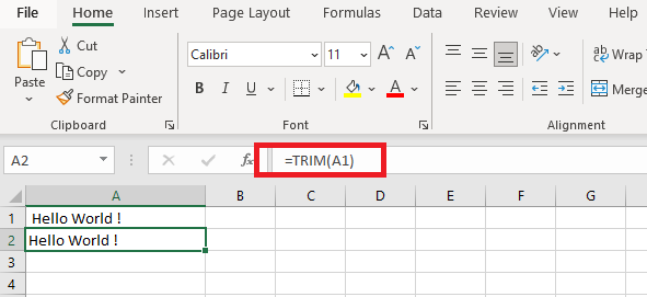
10 – TRIM()
TRIM: This formula removes any leading or trailing spaces from a piece of text. For example, if you had the cell A1 containing the text ” Hello World! “, you could use the formula =TRIM(A1) to remove the spaces and return the text “Hello World!”
11 – PROPER()
PROPER: This formula capitalizes the first letter of each word in a piece of text. For example, if you had the cell A1 containing the text ” hello world! “, you could use the formula =PROPER(A1) to return the text “Hello World!”
Hope you enjoyed those functions & examples.
Feel free to email me (ben@excelexposure.com) to let me know how you use them or any you think should be included!
Below is a brief overview of about 100 important Excel functions you should know, with links to detailed examples. We also have a large list of example formulas, a more complete list of Excel functions, and video training. If you are new to Excel formulas, see this introduction.
Note: Excel now includes Dynamic Array formulas, which offer important new functions.
Date and Time Functions
Excel provides many functions to work with dates and times.
NOW and TODAY
You can get the current date with the TODAY function and the current date and time with the NOW Function. Technically, the NOW function returns the current date and time, but you can format as time only, as seen below:

TODAY() // returns current date
NOW() // returns current time
Note: these are volatile functions and will recalculate with every worksheet change. If you want a static value, use date and time shortcuts.
DAY, MONTH, YEAR, and DATE
You can use the DAY, MONTH, and YEAR functions to disassemble any date into its raw components, and the DATE function to put things back together again.

=DAY("14-Nov-2018") // returns 14
=MONTH("14-Nov-2018") // returns 11
=YEAR("14-Nov-2018") // returns 2018
=DATE(2018,11,14) // returns 14-Nov-2018
HOUR, MINUTE, SECOND, and TIME
Excel provides a set of parallel functions for times. You can use the HOUR, MINUTE, and SECOND functions to extract pieces of a time, and you can assemble a TIME from individual components with the TIME function.

=HOUR("10:30") // returns 10
=MINUTE("10:30") // returns 30
=SECOND("10:30") // returns 0
=TIME(10,30,0) // returns 10:30
DATEDIF and YEARFRAC
You can use the DATEDIF function to get time between dates in years, months, or days. DATEDIF can also be configured to get total time in «normalized» denominations, i.e. «2 years and 6 months and 27 days».

Use YEARFRAC to get fractional years:

=YEARFRAC("14-Nov-2018","10-Jun-2021") // returns 2.57
EDATE and EOMONTH
A common task with dates is to shift a date forward (or backward) by a given number of months. You can use the EDATE and EOMONTH functions for this. EDATE moves by month and retains the day. EOMONTH works the same way, but always returns the last day of the month.

EDATE(date,6) // 6 months forward
EOMONTH(date,6) // 6 months forward (end of month)
WORKDAY and NETWORKDAYS
To figure out a date n working days in the future, you can use the WORKDAY function. To calculate the number of workdays between two dates, you can use NETWORKDAYS.

WORKDAY(start,n,holidays) // date n workdays in future
Video: How to calculate due dates with WORKDAY

NETWORKDAYS(start,end,holidays) // number of workdays between dates
Note: Both functions automatically skip weekends (Saturday and Sunday) and will also skip holidays, if provided. If you need more flexibility on what days are considered weekends, see the WORKDAY.INTL function and NETWORKDAYS.INTL function.
WEEKDAY and WEEKNUM
To figure out the day of week from a date, Excel provides the WEEKDAY function. WEEKDAY returns a number between 1-7 that indicates Sunday, Monday, Tuesday, etc. Use the WEEKNUM function to get the week number in a given year.

=WEEKDAY(date) // returns a number 1-7
=WEEKNUM(date) // returns week number in year
Engineering
CONVERT
Most Engineering functions are pretty technical…you’ll find a lot of functions for complex numbers in this section. However, the CONVERT function is quite useful for everyday unit conversions. You can use CONVERT to change units for distance, weight, temperature, and much more.

=CONVERT(72,"F","C") // returns 22.2
Information Functions
ISBLANK, ISERROR, ISNUMBER, and ISFORMULA
Excel provides many functions for checking the value in a cell, including ISNUMBER, ISTEXT, ISLOGICAL, ISBLANK, ISERROR, and ISFORMULA These functions are sometimes called the «IS» functions, and they all return TRUE or FALSE based on a cell’s contents.

Excel also has ISODD and ISEVEN functions that will test a number to see if it’s even or odd.
By the way, the green fill in the screenshot above is applied automatically with a conditional formatting formula.
Logical Functions
Excel’s logical functions are a key building block of many advanced formulas. Logical functions return the boolean values TRUE or FALSE. If you need a primer on logical formulas, this video goes through many examples.
AND, OR and NOT
The core of Excel’s logical functions are the AND function, the OR function, and the NOT function. In the screen below, each of these function is used to run a simple test on the values in column B:

=AND(B5>3,B5<9)
=OR(B5=3,B5=9)
=NOT(B5=2)
- Video: How to build logical formulas
- Guide: 50 examples of formula criteria
IFERROR and IFNA
The IFERROR function and IFNA function can be used as a simple way to trap and handle errors. In the screen below, VLOOKUP is used to retrieve cost from a menu item. Column F contains just a VLOOKUP function, with no error handling. Column G shows how to use IFNA with VLOOKUP to display a custom message when an unrecognized item is entered.

=VLOOKUP(E5,menu,2,0) // no error trapping
=IFNA(VLOOKUP(E5,menu,2,0),"Not found") // catch errors
Whereas IFNA only catches an #N/A error, the IFERROR function will catch any formula error.
IF and IFS functions
The IF function is one of the most used functions in Excel. In the screen below, IF checks test scores and assigns «pass» or «fail»:

Multiple IF functions can be nested together to perform more complex logical tests.
New in Excel 2019 and Excel 365, the IFS function can run multiple logical tests without nesting IFs.

=IFS(C5<60,"F",C5<70,"D",C5<80,"C",C5<90,"B",C5>=90,"A")
Lookup and Reference Functions
VLOOKUP and HLOOKUP
Excel offers a number of functions to lookup and retrieve data. Most famous of all is VLOOKUP:

=VLOOKUP(C5,$F$5:$G$7,2,TRUE)
More: 23 things to know about VLOOKUP.
HLOOKUP works like VLOOKUP, but expects data arranged horizontally:

=HLOOKUP(C5,$G$4:$I$5,2,TRUE)
INDEX and MATCH
For more complicated lookups, INDEX and MATCH offers more flexibility and power:

=INDEX(C5:E12,MATCH(H4,B5:B12,0),MATCH(H5,C4:E4,0))
Both the INDEX function and the MATCH function are powerhouse functions that turn up in all kinds of formulas.
More: How to use INDEX and MATCH
LOOKUP
The LOOKUP function has default behaviors that make it useful when solving certain problems. LOOKUP assumes values are sorted in ascending order and always performs an approximate match. When LOOKUP can’t find a match, it will match the next smallest value. In the example below we are using LOOKUP to find the last entry in a column:

ROW and COLUMN
You can use the ROW function and COLUMN function to find row and column numbers on a worksheet. Notice both ROW and COLUMN return values for the current cell if no reference is supplied:

The row function also shows up often in advanced formulas that process data with relative row numbers.
ROWS and COLUMNS
The ROWS function and COLUMNS function provide a count of rows in a reference. In the screen below, we are counting rows and columns in an Excel Table named «Table1».

Note ROWS returns a count of data rows in a table, excluding the header row. By the way, here are 23 things to know about Excel Tables.
HYPERLINK
You can use the HYPERLINK function to construct a link with a formula. Note HYPERLINK lets you build both external links and internal links:

=HYPERLINK(C5,B5)
GETPIVOTDATA
The GETPIVOTDATA function is useful for retrieving information from existing pivot tables.

=GETPIVOTDATA("Sales",$B$4,"Region",I6,"Product",I7)
CHOOSE
The CHOOSE function is handy any time you need to make a choice based on a number:

=CHOOSE(2,"red","blue","green") // returns "blue"
Video: How to use the CHOOSE function
TRANSPOSE
The TRANSPOSE function gives you an easy way to transpose vertical data to horizontal, and vice versa.

{=TRANSPOSE(B4:C9)}
Note: TRANSPOSE is a formula and is, therefore, dynamic. If you just need to do a one-time transpose operation, use Paste Special instead.
OFFSET
The OFFSET function is useful for all kinds of dynamic ranges. From a starting location, it lets you specify row and column offsets, and also the final row and column size. The result is a range that can respond dynamically to changing conditions and inputs. You can feed this range to other functions, as in the screen below, where OFFSET builds a range that is fed to the SUM function:

=SUM(OFFSET(B4,1,I4,4,1)) // sum of Q3
INDIRECT
The INDIRECT function allows you to build references as text. This concept is a bit tricky to understand at first, but it can be useful in many situations. Below, we are using INDIRECT to get values from cell A1 in 5 different worksheets. Each reference is dynamic. If a sheet name changes, the reference will update.

=INDIRECT(B5&"!A1") // =Sheet1!A1
The INDIRECT function is also used to «lock» references so they won’t change, when rows or columns are added or deleted. For more details, see linked examples at the bottom of the INDIRECT function page.
Caution: both OFFSET and INDIRECT are volatile functions and can slow down large or complicated spreadsheets.
STATISTICAL Functions
COUNT and COUNTA
You can count numbers with the COUNT function and non-empty cells with COUNTA. You can count blank cells with COUNTBLANK, but in the screen below we are counting blank cells with COUNTIF, which is more generally useful.

=COUNT(B5:F5) // count numbers
=COUNTA(B5:F5) // count numbers and text
=COUNTIF(B5:F5,"") // count blanks
COUNTIF and COUNTIFS
For conditional counts, the COUNTIF function can apply one criteria. The COUNTIFS function can apply multiple criteria at the same time:

=COUNTIF(C5:C12,"red") // count red
=COUNTIF(F5:F12,">50") // count total > 50
=COUNTIFS(C5:C12,"red",D5:D12,"TX") // red and tx
=COUNTIFS(C5:C12,"blue",F5:F12,">50") // blue > 50
Video: How to use the COUNTIF function
SUM, SUMIF, SUMIFS
To sum everything, use the SUM function. To sum conditionally, use SUMIF or SUMIFS. Following the same pattern as the counting functions, the SUMIF function can apply only one criteria while the SUMIFS function can apply multiple criteria.

=SUM(F5:F12) // everything
=SUMIF(C5:C12,"red",F5:F12) // red only
=SUMIF(F5:F12,">50") // over 50
=SUMIFS(F5:F12,C5:C12,"red",D5:D12,"tx") // red & tx
=SUMIFS(F5:F12,C5:C12,"blue",F5:F12,">50") // blue & >50
Video: How to use the SUMIF function
AVERAGE, AVERAGEIF, and AVERAGEIFS
Following the same pattern, you can calculate an average with AVERAGE, AVERAGEIF, and AVERAGEIFS.

=AVERAGE(F5:F12) // all
=AVERAGEIF(C5:C12,"red",F5:F12) // red only
=AVERAGEIFS(F5:F12,C5:C12,"red",D5:D12,"tx") // red and tx
MIN, MAX, LARGE, SMALL
You can find largest and smallest values with MAX and MIN, and nth largest and smallest values with LARGE and SMALL. In the screen below, data is the named range C5:C13, used in all formulas.

=MAX(data) // largest
=MIN(data) // smallest
=LARGE(data,1) // 1st largest
=LARGE(data,2) // 2nd largest
=LARGE(data,3) // 3rd largest
=SMALL(data,1) // 1st smallest
=SMALL(data,2) // 2nd smallest
=SMALL(data,3) // 3rd smallest
Video: How to find the nth smallest or largest value
MINIFS, MAXIFS
The MINIFS and MAXIFS. These functions let you find minimum and maximum values with conditions:

=MAXIFS(D5:D15,C5:C15,"female") // highest female
=MAXIFS(D5:D15,C5:C15,"male") // highest male
=MINIFS(D5:D15,C5:C15,"female") // lowest female
=MINIFS(D5:D15,C5:C15,"male") // lowest male
Note: MINIFS and MAXIFS are new in Excel via Office 365 and Excel 2019.
MODE
The MODE function returns the most commonly occurring number in a range:

=MODE(B5:G5) // returns 1
RANK
To rank values largest to smallest, or smallest to largest, use the RANK function:

Video: How to rank values with the RANK function
MATH Functions
ABS
To change negative values to positive use the ABS function.

=ABS(-134.50) // returns 134.50
RAND and RANDBETWEEN
Both the RAND function and RANDBETWEEN function can generate random numbers on the fly. RAND creates long decimal numbers between zero and 1. RANDBETWEEN generates random integers between two given numbers.

=RAND() // between zero and 1
=RANDBETWEEN(1,100) // between 1 and 100
ROUND, ROUNDUP, ROUNDDOWN, INT
To round values up or down, use the ROUND function. To force rounding up to a given number of digits, use ROUNDUP. To force rounding down, use ROUNDDOWN. To discard the decimal part of a number altogether, use the INT function.

=ROUND(11.777,1) // returns 11.8
=ROUNDUP(11.777) // returns 11.8
=ROUNDDOWN(11.777,1) // returns 11.7
=INT(11.777) // returns 11
MROUND, CEILING, FLOOR
To round values to the nearest multiple use the MROUND function. The FLOOR function and CEILING function also round to a given multiple. FLOOR forces rounding down, and CEILING forces rounding up.

=MROUND(13.85,.25) // returns 13.75
=CEILING(13.85,.25) // returns 14
=FLOOR(13.85,.25) // returns 13.75
MOD
The MOD function returns the remainder after division. This sounds boring and geeky, but MOD turns up in all kinds of formulas, especially formulas that need to do something «every nth time». In the screen below, you can see how MOD returns zero every third number when the divisor is 3:

SUMPRODUCT
The SUMPRODUCT function is a powerful and versatile tool when dealing with all kinds of data. You can use SUMPRODUCT to easily count and sum based on criteria, and you can use it in elegant ways that just don’t work with COUNTIFS and SUMIFS. In the screen below, we are using SUMPRODUCT to count and sum orders in March. See the SUMPRODUCT page for details and links to many examples.

=SUMPRODUCT(--(MONTH(B5:B12)=3)) // count March
=SUMPRODUCT(--(MONTH(B5:B12)=3),C5:C12) // sum March
SUBTOTAL
The SUBTOTAL function is an «aggregate function» that can perform a number of operations on a set of data. All told, SUBTOTAL can perform 11 operations, including SUM, AVERAGE, COUNT, MAX, MIN, etc. (see this page for the full list). The key feature of SUBTOTAL is that it will ignore rows that have been «filtered out» of an Excel Table, and, optionally, rows that have been manually hidden. In the screen below, SUBTOTAL is used to count and sum only the 7 visible rows in the table:

=SUBTOTAL(3,B5:B14) // returns 7
=SUBTOTAL(9,F5:F14) // returns 9.54
AGGREGATE
Like SUBTOTAL, the AGGREGATE function can also run a number of aggregate operations on a set of data and can optionally ignore hidden rows. The key differences are that AGGREGATE can run more operations (19 total) and can also ignore errors.
In the screen below, AGGREGATE is used to perform MIN, MAX, LARGE and SMALL operations while ignoring errors. Normally, the error in cell B9 would prevent these functions from returning a result. See this page for a full list of operations AGGREGATE can perform.

=AGGREGATE(4,6,values) // MAX ignore errors, returns 100
=AGGREGATE(5,6,values) // MIN ignore errors, returns 75
TEXT Functions
LEFT, RIGHT, MID
To extract characters from the left, right, or middle of text, use LEFT, RIGHT, and MID functions:

=LEFT("ABC-1234-RED",3) // returns "ABC"
=MID("ABC-1234-RED",5,4) // returns "1234"
=RIGHT("ABC-1234-RED",3) // returns "RED"
LEN
The LEN function will return the length of a text string. LEN shows up in a lot of formulas that count words or characters.

FIND, SEARCH
To look for specific text in a cell, use the FIND function or SEARCH function. These functions return the numeric position of matching text, but SEARCH allows wildcards and FIND is case-sensitive. Both functions will throw an error when text is not found, so wrap in the ISNUMBER function to return TRUE or FALSE (example here).

=FIND("Better the devil you know","devil") // returns 12
=SEARCH("This is not my beautiful wife","bea*") // returns 12
REPLACE, SUBSTITUTE
To replace text by position, use the REPLACE function. To replace text by matching, use the SUBSTITUTE function. In the first example, REPLACE removes the two asterisks (**) by replacing the first two characters with an empty string («»). In the second example, SUBSTITUTE removes all hash characters (#) by replacing «#» with «».

=REPLACE("**Red",1,2,"") // returns "Red"
=SUBSTITUTE("##Red##","#","") // returns "Red"
CODE, CHAR
To figure out the numeric code for a character, use the CODE function. To translate the numeric code back to a character, use the CHAR function. In the example below, CODE translates each character in column B to its corresponding code. In column F, CHAR translates the code back to a character.

=CODE("a") // returns 97
=CHAR(97) // returns "a"
Video: How to use the CODE and CHAR functions
TRIM, CLEAN
To get rid of extra space in text, use the TRIM function. To remove line breaks and other non-printing characters, use CLEAN.

=TRIM(A1) // remove extra space
=CLEAN(A1) // remove line breaks
Video: How to clean text with TRIM and CLEAN
CONCAT, TEXTJOIN, CONCATENATE
New in Excel via Office 365 are CONCAT and TEXTJOIN. The CONCAT function lets you concatenate (join) multiple values, including a range of values without a delimiter. The TEXTJOIN function does the same thing, but allows you to specify a delimiter and can also ignore empty values.

=TEXTJOIN(",",TRUE,B4:H4) // returns "red,blue,green,pink,black"
=CONCAT(B7:H7) // returns "8675309"
Excel also provides the CONCATENATE function, but it doesn’t offer special features. I wouldn’t bother with it and would instead concatenate directly with the ampersand (&) character in a formula.
EXACT
The EXACT function allows you to compare two text strings in a case-sensitive manner.

UPPER, LOWER, PROPER
To change the case of text, use the UPPER, LOWER, and PROPER function

=UPPER("Sue BROWN") // returns "SUE BROWN"
=LOWER("Sue BROWN") // returns "sue brown"
=PROPER("Sue BROWN") // returns "Sue Brown"
Video: How to change case with formulas
TEXT
Last but definitely not least is the TEXT function. The text function lets you apply number formatting to numbers (including dates, times, etc.) as text. This is especially useful when you need to embed a formatted number in a message, like «Sale ends on [date]».

=TEXT(B5,"$#,##0.00")
=TEXT(B6,"000000")
="Save "&TEXT(B7,"0%")
="Sale ends "&TEXT(B8,"mmm d")
More: Detailed examples of custom number formatting.
Dynamic Array functions
Dynamic arrays are new in Excel 365, and are a major upgrade to Excel’s formula engine. As part of the dynamic array update, Excel includes new functions which directly leverage dynamic arrays to solve problems that are traditionally hard to solve with conventional formulas. If you are using Excel 365, make sure you are aware of these new functions:
| Function | Purpose |
|---|---|
| FILTER | Filter data and return matching records |
| RANDARRAY | Generate array of random numbers |
| SEQUENCE | Generate array of sequential numbers |
| SORT | Sort range by column |
| SORTBY | Sort range by another range or array |
| UNIQUE | Extract unique values from a list or range |
| XLOOKUP | Modern replacement for VLOOKUP |
| XMATCH | Modern replacement for the MATCH function |
Video: New dynamic array functions in Excel (about 3 minutes).
Quick navigation
ABS, AGGREGATE, AND, AVERAGE, AVERAGEIF, AVERAGEIFS, CEILING, CHAR, CHOOSE, CLEAN, CODE, COLUMN, COLUMNS, CONCAT, CONCATENATE, CONVERT, COUNT, COUNTA, COUNTBLANK, COUNTIF, COUNTIFS, DATE, DATEDIF, DAY, EDATE, EOMONTH, EXACT, FIND, FLOOR, GETPIVOTDATA, HLOOKUP, HOUR, HYPERLINK, IF, IFERROR, IFNA, IFS, INDEX, INDIRECT, INT, ISBLANK, ISERROR, ISEVEN, ISFORMULA, ISLOGICAL, ISNUMBER, ISODD, ISTEXT, LARGE, LEFT, LEN, LOOKUP, LOWER, MATCH, MAX, MAXIFS, MID, MIN, MINIFS, MINUTE, MOD, MODE, MONTH, MROUND, NETWORKDAYS, NOT, NOW, OFFSET, OR, PROPER, RAND, RANDBETWEEN, RANK, REPLACE, RIGHT, ROUND, ROUNDDOWN, ROUNDUP, ROW, ROWS, SEARCH, SECOND, SMALL, SUBSTITUTE, SUBTOTAL, SUM, SUMIF, SUMIFS, SUMPRODUCT, TEXT, TEXTJOIN, TIME, TODAY, TRANSPOSE, TRIM, UPPER, VLOOKUP, WEEKDAY, WEEKNUM, WORKDAY, YEAR, YEARFRAC
41 EXCEL EXPERTS WEIGH IN
Brought to You by AutomateExcel.com
Microsoft Excel has hundreds of functions. Even experienced Excel users can find themselves wondering if they are using the best Excel formulas for their projects.
With that in mind, we polled 41 Excel experts and asked them the question: What is the most under-used Excel function? Their answers are listed below.
Want to master the 30 most-used Excel Functions?
CHOOSE Function — 4 Votes
The CHOOSE function was my vote for the most under-used Excel function. It’s easy to understand and very powerful. CHOOSE allows you to select one of up to 254 values or options based on an index number. — Michael from Excel Bytes.
As John from How to Excel implies, this might not sound like much, but in the right circumstance it can be very powerful: I remember when I first met CHOOSE. I thought to myself, «Wow, what a boring function. All it does is choose an item in your list based on an index number. Doesn’t INDEX already do that?» It looks like a very simple function at the outset, but when you combine it with other formulas it can be quite powerful.
My favorite use of the CHOOSE Functions is this: Let’s say you have 4 worksheets: a Forecast sheet, a Budget sheet, a Trailing 12 sheet, and a Summary sheet. On the Summary sheet, you use drop-downs to select which sheet’s data to show:

In the above example, the CHOOSE function allows you to read data from one of three sheets. Cell F$1 contains a MATCH function that looks to see what option was selected from the drop-down (drop-down currently reads «Budget») and returns the corresponding number, which is used by the CHOOSE function. You can see that by using the CHOOSE function you can select values from different sheets, while avoiding volatile functions like INDIRECT.
Lookup Formulas — VLOOKUP, HLOOKUP, INDEX, and MATCH — 5 Total Votes
The lookup functions are hands-down some of the most important Excel functions. You can’t claim to be an Excel expert without being proficient with these.
VLOOKUP & HLOOKUP
Laurent from ExcelMadeEasy says this about the Vlookup: Looking for data in a specific column, row, or a full table? Excel has a solution in the form of VLOOKUP and HLOOKUP functions.
The VLOOKUP allows you to search for a value in a column («V» for vertical) and return another value from that same row. The HLOOKUP allows you to search for a value in a row («H» for «horizontal») and return another value from that same column.

The VLOOKUP and HLOOKUP have two big limitations:
- The lookup column must be the left-most column in the data (or top-most row for a HLOOKUP). Often your data will not come in this format.
- In large workbooks, these lookup functions can take a very long time to run. Ole from Erlandsen Data Consulting says this: A little bit off-topic, but here is a function that I think is sometimes over-used or used in a wrong way: VLOOKUP. This function is extremely useful, but can sometimes cause the calculations in a workbook to slow down to a crawl when used with large data sources and/or in a lot of cells. An example: a workbook that took 5-10 minutes to calculate because of excessive use of the VLOOKUP function, took 7 seconds to calculate after sorting the data sources and replacing VLOOKUP with MATCH and INDEX functions.
NDEX & MATCH
The MATCH function looks up a value in an array of cells and returns the position # where that value is found.
The INDEX function returns a value from an array of cells based on the provided position #.
Together these functions can be used to simulate a VLOOKUP, only with more flexibility. Othniel from Excellent Ones Consulting says this These two functions together are more powerful than the traditional VLOOKUP In a VLOOKUP formula the field to be matched must be in the first column of your data set. Using a combination of Index and match removes those limitation. This adds more flexibility to the user.

Alan from ComputerGaga notes some other advanced uses of the INDEX function: However other awesome uses include to return the last value from a row or column, to create dynamic ranges and its use with form controls for interactive charts and dashboards.
Match Multiple Criteria with a Formula
These functions also allow you to match multiple criteria. However, the formula is quite complicated!
Marcus Small explains My favourite function to rip out in any of my courses is the combination of INDEX, MATCH, and INDEX. This powerful three part formula allows you to return a match based on multiple criteria. It avoids the concatenation of data with the inevitable use of VLOOKUP and it does not need to be in the form of an array formulation. One caveat, I only use this formula when I am wanting to return TEXT based on multiple criteria, as Excel has SUMIFS and SUMPRODUCT available to deal with multi criteria calculation returns. Quite simply it is formulaic brilliance!!!
The syntax is
Index(result column, match(1, index((criteria range=criteria)*(criteria range2 =criteria2),0),0))
The formula works as it is attempting to match the true condition to the specified criteria. In the above example there is 2 criteria however you could have 3, 4, 5 etc. The secret lies in the 1 part of the MATCH formula. If a match is made in the second INDEX, Excel produces a 1, if no match to the corresponding cell in the second INDEX criteria, Excel produces a zero, so 1 x 0 = 0. Excel continues until 2 matches are made 1 x 1 = 1 and the row where this occurs is then pushed into the first INDEX formula (INDEX(Result Column) to return the value of the row in the result column. It is a marvellous formula which can easily be extended with little effort. Here is 3 criteria:
Index(result column, match(1, index((criteria range=criteria)*(criteria range2 =criteria2)*(criteria range3 =criteria3),0),0))
Now the structure of a file can be preserved without resorting to adding a column to concatenate data so it can be used as LOOKUP criteria.
IFERROR Function — 3 Votes
IFERROR was one of my top choices for the most under-used function in Excel. It’s easy to use, and makes your spreadsheets look much more professional.
Janet from Savvy Spreadsheets describes it’s usefulness: I’ve seen too many reports with ugly # errors in them. The IFERROR function can be wrapped around a formula to quickly and easily hide those errors, by returning something else such as a blank or zero.
If you submit a spreadsheet to a client or superior filled with formula errors, it makes you look bad. Did you even review those errors? Are they valid errors or not? IFERROR makes a huge difference in how the quality of your work is perceived.

Joe from Excel by Joe describes how to use it: IFERROR is very easy to set up and it can easily eliminate all error messages from your function results. I use it all the time when building spreadsheets. To use it, simply insert whatever function you have written into the first part of the IFERROR and then put a comma and then enter what you want shown if there’s an error. For example, if you want to display a zero whenever your function, A1/A2 has an error, use this code : =IFERROR(A1/A2,0)
Zach from Data Automation Professionals notes that IFERROR was a new function for Excel 2007. Microsoft added this function to save you the hassle of using =IF(ISERROR( and needing to enter the same formula twice.
SUMPRODUCT Function — 3 Votes
The SUMPRODUCT Function sums the products of multiple arrays. The simplest example is calculating total sales revenue based on # of Units Sold and Price per Unit:

SUMPRODUCT can also be used to perform advanced calculations. By creating columns with 1 or 0, you can create «if» conditions where records are only counted if they meet certain criteria (note: multiplying by 0 excludes the record from the SUMPRODUCT, multiplying by 1 includes it). As Ashish says, SUMPRODUCT allows one to specify multiple AND/OR conditions. My Excel Online notes that: this technique is like using SUMIFS on steroids.
Glen from Need a Spreadsheet is right when he says, It takes a while to get your head around SUMPRODUCT, but when you do it gives you enormous power and flexibility.
CONCATENATE, CONCAT, & TEXTJOIN Functions — 2 Votes
Juan from Excel MOOC and Mourad from Excel-Translator voted for CONCATENATE / CONCAT. The CONCATENATE function merges strings of text together. The CONCAT function is a newer version that does the same thing except with a shorter name (less typing the better!). Here is an example of merging text with a space (» «) in between:

The big downside to CONCATENATE is that you can’t merge an array of cells together. Instead, you must manually select each cell to merge. Microsoft fixed this problem with the new (for Excel 2016) function: TEXTJOIN:

Notice the syntax: First you enter the deliminator (we chose a space » «). Next you enter TRUE/FALSE to decide if blank cells are counted, and last you enter the range to merge.
SIGN Function — 2 Votes
From Amiq Khan’s blog: The Excel SIGN function checks the sign of a number and gives result of 1 if the number is positive, 0 if number is zero and -1 if the number is negative.
When would you use this?
Bill Jelen is a big fan of using the SIGN Function with the Up/Flat/Down icon set:

Bill says: In Row 1, negative numbers like -24 in I1 get an up indicator. Use the SIGN Function to make sure you only get 1,0, or -1 and the icons behave.
SUMIFS & More — 2 Votes
Alex Powers from It’s Not About the Cell and Joseph from Spreadsheets Made Easy both voted for the SUMIFS, COUNTIFS, and, AVERAGEIFS Functions. These functions allow you to perform the desired calculations (sum, count, or average), only on data that meet certain criteria.

Also, new for Excel 2016 are the MAXIFS and MINIFS Functions (a life-saver for some of the work that I’ve done).
Alex and Joseph also noted that you can transform the basic SUM Function into a much more powerful SUMIFS with the use of «array» functions. Array functions are sometimes referred to as CSE (CTRL + SHIFT + ENTER) functions because when you enter the functions you must type CTRL + SHIFT + ENTER. With array functions, you can perform very complicated calculations, however they can be hard to create (or follow) for all but the most advanced Excel users. With that in mind, we won’t cover an example.
TEXT Function — 2 Votes
The TEXT Function allows you to display a number stored as text in a specified number format.
Brad Edgar described this example: In cell A1 you have the date 04-OCT-2017 and you want to reference that date in a string of text:
=»Today’s date is: » & A1
By default, Excel will show «Today’s date is: 43012» (43012 is the serial number corresponding to that date). Instead, to show the nicely formatted date use the TEXT Function:
=»Today’s date is: » & TEXT(A1,»DD-MMM-YYYY»)

Steve=True from Excel Dashboard Templates had another example:
If you want to display a number with leading zeroes (ex. a ZIP code):
IF and IFS (New for Excel 2016) — 2 Votes
The IF function is ubiquitous in all of coding, as Alex discusses here. It tests if a condition is met. If so, it does something, if not it does something else. You won’t get very far with Excel (or any coding language) without understanding this common function.

New for Excel 2016, Microsoft released the IFS function. Nick from Excel Spreadsheet Help says: With the IFS function you can now simplify one of the most common uses of the IF function: the dreaded nested IFs. If you use Excel frequently then at some point you’ve probably had to create a crazy long formula with multiple IF functions where it’s difficult to keep track of all the logic and commas. With the release of Excel 2016, the IFS function provides the same results as a nested IF formula but with a much simpler and easy to read method. IFS may be one of the most under-used Excel functions for now because it’s so new, but I think it’s use is going to spread rapidly once Excel users are aware of it existence!
Become an Excel Function Expert
Take our 100% free interactive tutorial on Excel functions. Master the 30 most-used Excel functions!
CONVERT — 2 Votes
From Charlie at Engineer Excel: CONVERT is a really efficient way to convert many different quantities like length, mass, volume, etc. between different sets of units. I find that many people (myself included before I found this function) «hard code» numbers into their spreadsheets in order to convert between unit systems. The CONVERT function eliminates the need to do that.
Kawser from Exceldemy provides a good example: Say I want to convert 100 Tones to Stones. See the image below.

It’s easy to convert almost any unit to other relevant unit using this Excel function.
SUBTOTAL Function — 1 Votes
Ben from Excel Exposure voted for the SUBTOTAL function saying: People generally don’t know what it does, or how to use it. Even while praising it now myself, I realize I don’t use it enough.
The SUBTOTAL Functions allows you to perform different calculations on a data set. You can see the list of options when you enter the function into Excel:

You might be asking yourself, why wouldn’t you just use the AVERAGE function if you want to average or the COUNT function if you want to count?
You would use SUBTOTAL when you might change which calculation you wish to view. For example, you create a summary sheet to summarize a very large data set. You create a drop-down to select what information to show. Without using the SUBTOTAL function, you would need to create each calculation individually, and the drop-down would select which to show. With SUBTOTAL, you can create one formula that reads the drop-down and performs the appropriate calculation.
The SUBTOTAL function can reduce your calculation speed and reduce the number of formulas needed.
DOLLARDE and DOLLARFR — 1 Votes
Vijay from E for Excel says: Though designed as financial functions, these perform great conversion routines. I, very often, use them for time to decimal conversions. For example, 1:30 hours is 1.5 hours in decimal.
=DOLLARDE(1.30,60)

To convert it back to 1:30
=DOLLARFR(1.5,60)
(Note, it converts decimals not time value i.e. why 1.3 has been used to convert into 1.5. Though the same you can achieve through multiplying by 24 in case of DOLLARDE and divide by 24 for DOLLARFR. Hence 1:30/24 will give 1.5 and 1.5/24 will give 1:30)
The impact is even more strong once you perform other odd conversions
Convert 6 feet 6 inches
=DOLLARDE(6.06,12)
Which is 6.5 i.e. 6 and half feet
Similarily 6.3 is 6.5 dozen if =DOLLARDE(6.5,6) i.e. 6 and half dozen
So, you can perform many odd conversions which can not be done by CONVERT function.
Date Functions — 1 `Votes
Erin from Time Saving Templates suggested the date functions: DAY, MONTH, and YEAR. These functions extract the day, month, or year number from a date. If you work with dates you should know and use these (easy to remember) functions.

I also recommend the EDATE, EOMONTH, and DATE Functions. EDATE and EOMONTH roll dates forward or back a number of months (EOMONTH then returns the last day of that month). DATE is used to create a date from a given day, month or, year.
When entering dates into Excel, use one input cell to provide the starting date or year, and calculate all other dates using these functions. This makes updating spreadsheets monthly or annually a breeze! No more manually editing hard-coded dates!
MMULT Function — 1 `Votes
Earlier we mentioned the SUMPRODUCT function. SUMPRODUCT allows you to sum the products of multiple arrays. The MMULT function can be used in a similar way. Oscar from Get Digital Help says MMULT allows you to do calculations like the SUMPRODUCT function but in a more granular way. SUMPRODUCT lets you multiply and then sum arrays, whereas the MMULT function lets you multiply and sum arrays row-wise or column-wise.
MMULT stands for Matrix Multiplication. If you have a strong math background, you’ll know exactly what it does:

It’s also an Array function (notice the brackets surrounding the formula above), which means you must use CTRL + SHIFT + ENTER when entering the formula.
INDIRECT Function — 1 `Votes
Abhilash from Excel to XL recommended the INDIRECT function. The INDIRECT Function allows you to «indirectly» reference cell ranges by treating the cell range as text.
To reference cell A1:
=INDIRECT(«A1»)
This is useful when you want to use formulas to determine which cell to reference. So instead of hard-coding «A1» into the formula above, you could reference a cell with formulas that output «A1», «B2», etc. This can be VERY useful when your desired ranges are on different worksheets.

Warning: INDIRECT is a «volatile» function, meaning it re-calculates every time Excel recalculates the workbook. They won’t slow your workbook down if you use a small number of them, but if you have large blocks of INDIRECT functions, you may start to notice a lag.
Often, you can avoid INDIRECTs with smart use of the CHOOSE and INDEX functions (see above).
LEN Function — 1 `Votes
The LEN Function counts the number of characters in a string of text. LEN can be useful when using other text functions such as LEFT, RIGHT, or MID.

Onur from Someka.net makes an outstanding point about using LEN to check for blank cells: LEN is the most reliable way to check blank cells.
Some of you may ask: «Hey, I use =IF(A1=»»,…) method for checking blank cells, why would I need the LEN function? Aren’t they the same?»
I prefer to use LEN for two reasons:
- When you copy and paste from other applications (word, access) blank cells are not counted as «real blank cells». (read more)
- Sometimes people enter space, line break, dot, or something similar to a blank cell, whether intentionally or accidentally. The workbooks need to account for this as well.
For these reasons to be on the very safe side I prefer to use LEN. In most cases, =IF(A1=»»,…) will do the work though.
OFFSET Function — 1 `Votes
Ismael from Excelforo voted for the OFFSET function. With the OFFSET function, you reference a cell by «offsetting» a certain number of rows and columns from a starting point. You can also resize the cell range to any number of rows and columns.

I’ve found the OFFSET function be extremely useful when coupled with VBA code that inserts and deletes rows and columns. By using the OFFSET, you can avoid #REF errors that appear when referenced cells are deleted.
Note: OFFSET is a «volatile function». Volatile functions recalculate each time Excel recalculates. If you have too many OFFSET functions, your workbook will slow down.
REPT Function — 1 `Votes
The REPT function allows you to repeat a string of text a certain number of times:

The true value of this function, however, lies in more creative uses as Crispo from CrispExcel points out: Although classified as a text function, REPT function does more than just repeating texts a number of times. For example, REPT is a perfect alternative to the slow calculating and complex Nested IF function. This is because REPT function can also act as a Logical Function returning an empty string if the number to return is zero. This ability to return an empty string makes it a perfect function for leaving comments within a cell instead of using N function.
REPT‘s ability to repeat characters also makes it perfect to create Mirror Charts (see below), Inline charts, Stem & Leaf Plots, Sparkline, star rating template and even the elusive FOMC dot plot chart.

CELL & GET Functions — 1 `Votes
The team at Spreadsheet Detective suggested the GET & CELL functions. The GET function is an old XL4 function that can’t be used in the same way as a normal Excel function. If you’re interested in using this function, here is more information (warning: It’s complicated).
The function can return useful information about a cell: color, row height, and much more. However, all of this can also be accomplished using VBA or some of the functionality can be accomplished with the newer CELL function.
The CELL function can return the following information about a cell:
Simply define the information you want to see and which cell you want to test!
MOD Function — 1 `Votes
The MOD function returns the remainder of two numbers after division. Why is this useful? You can easily determine odd or even numbered rows (for alternate row shading) and, more generally, split data into separate groups.
Jorge from Power Spreadsheets says: The main reason I find MOD useful is because of how it allows you to break a group of items into different groups. I commonly use MOD in 2 contexts: (i) in conditional formatting formulas, such as formatting alternate rows or columns; or (ii) to classify entries or values into different groups, which allows you to work with subsets or them (for example, working with odd or even numbers, or entries located every nth cell).

GETPIVOTDATA — 1 `Votes
Debra from Contextures.com recommended the GETPIVOTDATA function: A GETPIVOTDATA formula is automatically created if you link to a PivotTable Value cell. Don’t turn that feature off! Learn how to tweak the formula, so it will pull out the pivot table data that you need.
Her site has an excellent page on the GETPIVOTDATA Function. Visit it to learn more.

User-Defined Functions — 1 `Votes
User-Defined Functions (UDFs) are custom functions created in VBA. If Excel doesn’t have a function that you need, you can create your own in VBA. Obviously, VBA isn’t for everyone, but if you are familiar with VBA, you might want to keep UDFs in mind. Jon from Vertex42 talks about UDFs: I think that custom user-defined functions may be underutilized. While there are many reasons why you might not want to use VBA within a spreadsheet, it is pretty simple to create your own add-in and populate it with custom functions that help speed up what you do in Excel. I avoid using custom functions in spreadsheets that I share with other people, but there are many custom functions that I use that allow me to easily do things I might not otherwise be able to do. Using the VB date functions to work with dates prior to 1900 is an example.
Text to Columns — 1 `Votes
Text to Columns isn’t an Excel function, but it is a very powerful Excel tool that can be used instead of using Excel text functions. The team at TestsTestsTests.com says this: Excel users (that don’t know better) can spend hours manually separating and moving data from a single column to adjacent columns using copy/cut and paste or Excel text functions like LEFT, RIGHT, MID, etc.. A column may contain names, surnames, and/or dates of births that needs to be separated. A surprisingly quick and easy way of doing this is to use Text to Columns located in the Data Tools group under the Data tab of the Excel Ribbon. Text to Columns provides multiple options to separate the data, including by delimiters such as spaces or commas, or by a fixed width, allowing you to separate the data visually. This tool becomes especially useful when data is copied and pasted from other applications, such as tables in Microsoft Word, .csv (comma separated values) files, and more.

Flash Fill — 1 `Votes
Just like Text to Columns, Flash Fill isn’t an Excel function, but it is an under-used feature of Excel that can help alleviate the need for complex Excel formulas. The team over at Yoda Learning said this: Simply enter a pattern in the first several cells. Go to Data > Flash Fill (CTRL + E) and Excel will calculate the algorithm for the rest of the column.
Note: Generally, you would use this when you have a column of fully-populated data and you would like to create a second column based off of the first. For example, in the second column you would like to add «test» in front of the text from the first column. Instead of creating a formula to do so, you would manually enter the values in and then go to Flash Fill to populate the rest of the column.
You might notice that Excel suggests this automatically for you. In the Options menu you can toggle whether automatic Flash Fill is enabled or not.

Become an Excel Function Expert
Take our 100% free interactive tutorial on Excel functions. Master the 30 most-used Excel functions!