
Watch this video to learn how to create more complex formulas using multiple operators, cell references, and functions.
Want more?
Use AutoSum to sum numbers
Sum numbers by creating a formula
Now, we’ll create more complex formulas using multiple operators, cell references, and functions.
We are going to calculate the sales commission based off of the net revenue.
To do this, I take the Sales Price and subtract from it the Cost of goods sold.
This is in parentheses to ensure it occurs first.
I then multiply the Net profit by the Commission percentage in B4, 3%.
This returns the commission.
Let’s take a look at how this works in a formula.
Because the cell references are in parentheses, first the cost of goods sold is subtracted from the sales price.
This returns a Net profit of $3200.
This is then multiplied by 3%, returning a commission of $96.
Now, we are going to determine the Weighted scores for students.
By Weighted scores, I mean that different tests account for a different percentage of the students’ final grade.
Tests 1 and 2, each account for 10%, and the mid-term and final tests, each account for 40%.
To do this, I multiply the Test 1 score for Bob by its Weight.
I press F4 after I select the Weight value in B3, so that when I copy the formula, the Weight for Test 1 will always remain cell B3.
This is referred to as Absolute Cell Reference.
I then add Bob’s Mid-term score multiplied by its Weight in B4, and press F4 again.
I follow the same steps for Test 2 and the Final test.
To copy the formula, I click the cell, put the mouse pointer over the bottom right-hand corner of the cell until I get a black + sign, click the left mouse button, and drag the border to the right.
Here are the weighted scores for the students.
Let’s take a look at what’s happening in this formula for Bob’s Weighted score.
Each of the test scores and their weights are multiplied, resulting in this formula.
Then the numbers are added together, resulting in 74.5.
What’s the value returned by this formula? First, we do the inner most parentheses, 5 minus 3 is 2, resulting in this formula.
Next, we do the remaining parentheses, 10 times 2 is 20 and 1 minus 4 is -3, resulting in this formula.
Now, we do multiplication and division, from left to right.
6 times 20 is 120, divided by 3 is 40, resulting in this formula.
Lastly, we do addition and subtraction from left to right. 4 + 40 is 44, — 3 is 41.
You can use functions in formulas with multiple operators, including nested parentheses.
Functions and cell references are evaluated and treated as their resulting numbers.
The parentheses that follow a function name act only as a container for the function’s arguments, such as numbers or cell references, and don’t affect the order of operations in a formula.
Let’s take a look at what’s happening in this formula.
The functions and cell references are evaluated, resulting in this formula. The operations in parentheses occur first, resulting in a formula of 12 minus 3, and this is 9.
Now, you have a good idea about how to do basic math in Excel.
Of course, there’s more to learn.
So, check out the course summary at the end, and best of all, explore Excel 2013 on your own.
Самая популярная программа для работы с электронными таблицами «Microsoft Excel» упростила жизнь многим пользователям, позволив производить любые расчеты с помощью формул. Она способна автоматизировать даже самые сложные вычисления, но для этого нужно знать принципы работы с формулами. Мы подготовили самую подробную инструкцию по работе с Эксель. Не забудьте сохранить в закладки 😉
Содержание
-
Кому важно знать формулы Excel и где выучить основы.
-
Элементы, из которых состоит формула в Excel.
-
Основные виды.
-
Примеры работ, которые можно выполнять с формулами.
-
22 формулы в Excel, которые облегчат жизнь.
-
Использование операторов.
-
Использование ссылок.
-
Использование имён.
-
Использование функций.
-
Операции с формулами.
-
Как в формуле указать постоянную ячейку.
-
Как поставить «плюс», «равно» без формулы.
-
Самые распространенные ошибки при составлении формул в редакторе Excel.
-
Коды ошибок при работе с формулами.
-
Отличие в версиях MS Excel.
-
Заключение.
Кому важно знать формулы Excel и где изучить основы
Excel — эффективный помощник бухгалтеров и финансистов, владельцев малого бизнеса и даже студентов. Менеджеры ведут базы клиентов, а маркетологи считают в таблицах медиапланы. Аналитики с помощью эксель формул обрабатывают большие объемы данных и строят гипотезы.
Эксель довольно сложная программа, но простые функции и базовые формулы можно освоить достаточно быстро по статьям и видео-урокам. Однако, если ваша профессиональная деятельность подразумевает работу с большим объемом данных и требует глубокого изучения возможностей Excel — стоит пройти специальные курсы, например тут или тут.
Элементы, из которых состоит формула в Excel
Формулы эксель: основные виды
Формулы в Excel бывают простыми, сложными и комбинированными. В таблицах их можно писать как самостоятельно, так и с помощью интегрированных программных функций.
Простые
Позволяют совершить одно простое действие: сложить, вычесть, разделить или умножить. Самой простой является формула=СУММ.
Например:
=СУММ (A1; B1) — это сумма значений двух соседних ячеек.
=СУММ (С1; М1; Р1) — сумма конкретных ячеек.
=СУММ (В1: В10) — сумма значений в указанном диапазоне.
Сложные
Это многосоставные формулы для более продвинутых пользователей. В данную категорию входят ЕСЛИ, СУММЕСЛИ, СУММЕСЛИМН. О них подробно расскажем ниже.
Комбинированные
Эксель позволяет комбинировать несколько функций: сложение + умножение, сравнение + умножение. Это удобно, когда, например, нужно вычислить сумму двух чисел, и, если результат будет больше 100, его нужно умножить на 3, а если меньше — на 6.
Выглядит формула так ↓
=ЕСЛИ (СУММ (A1; B1)<100; СУММ (A1; B1)*3;(СУММ (A1; B1)*6))
Встроенные
Новичкам удобнее пользоваться готовыми, встроенными в программу формулами вместо того, чтобы писать их вручную. Чтобы найти нужную формулу:
-
кликните по нужной ячейке таблицы;
-
нажмите одновременно Shift + F3;
-
выберите из предложенного перечня нужную формулу;
-
в окошко «Аргументы функций» внесите свои данные.
Примеры работ, которые можно выполнять с формулами
Разберем основные действия, которые можно совершить, используя формулы в таблицах Эксель и рассмотрим полезные «фишки» для упрощения работы.
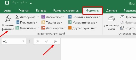
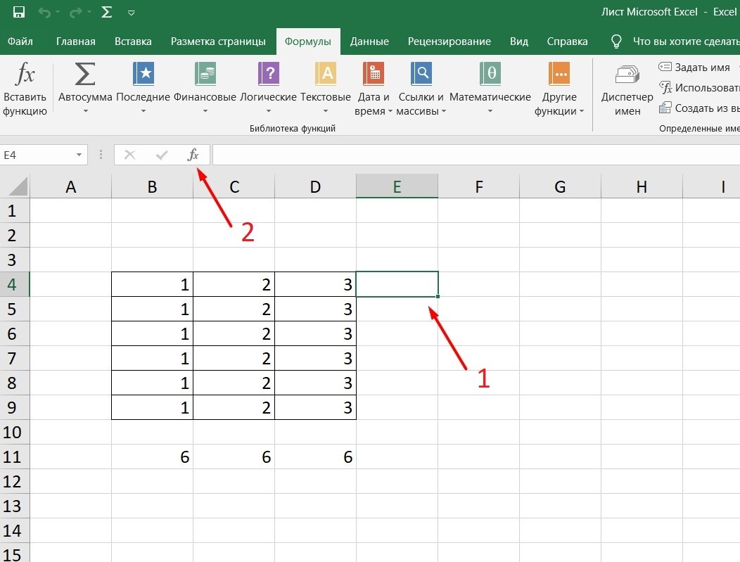
Поиск перечня доступных функций
Перейдите в закладку «Формулы» / «Вставить функцию». Или сразу нажмите на кнопочку «Fx».
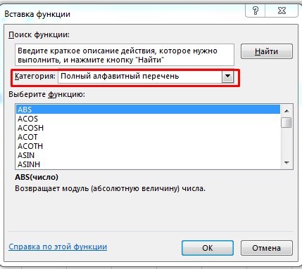
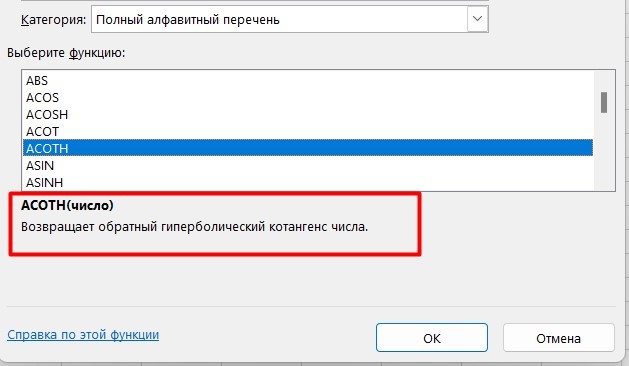
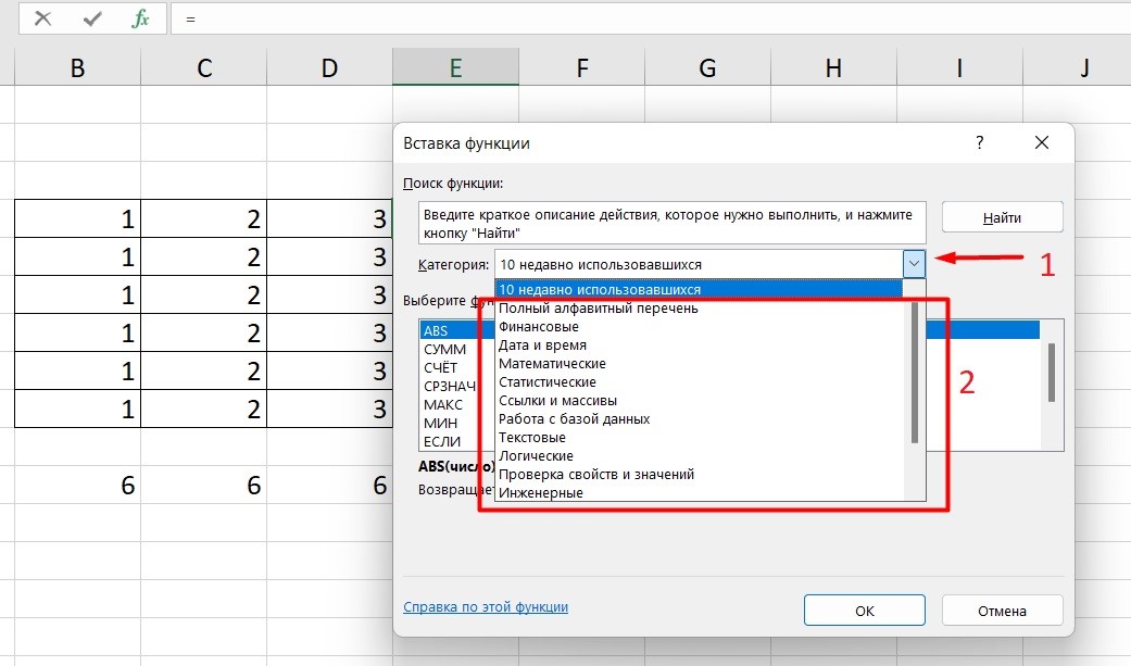
Выберите в категории «Полный алфавитный перечень», после чего в списке отобразятся все доступные эксель-формулы.
Выберите любую формулу и прочитайте ее описание. А если хотите изучить ее более детально, нажмите на «Справку» ниже.
Вставка функции в таблицу
Вы можете сами писать функции в Excel вручную после «=», или использовать меню, описанное выше. Например, выбрав СУММ, появится окошко, где нужно ввести аргументы (кликнуть по клеткам, значения которых собираетесь складывать):
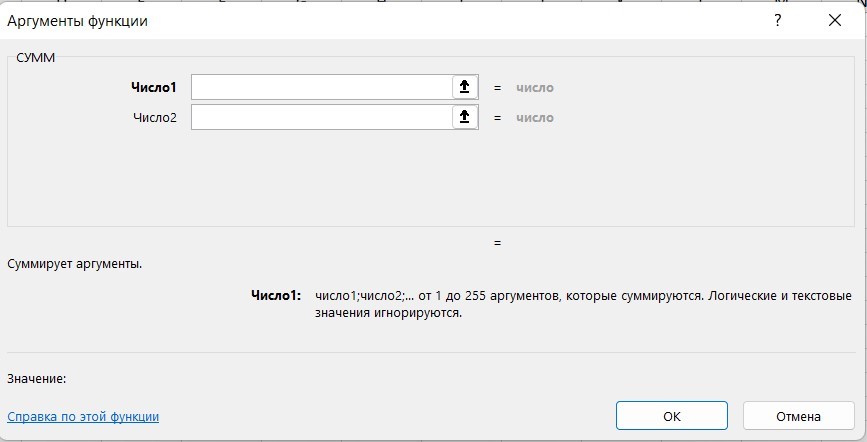
После этого в таблице появится формула в стандартном виде. Ее можно редактировать при необходимости.
Использование математических операций
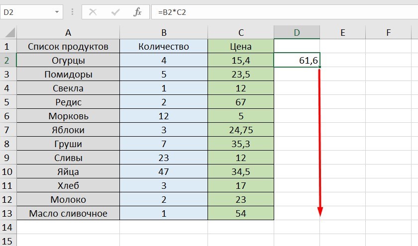
Начинайте с «=» в ячейке и применяйте для вычислений любые стандартные знаки «*», «/», «^» и т.д. Можно написать номер ячейки самостоятельно или кликнуть по ней левой кнопкой мышки. Например: =В2*М2. После нажатия Enter появится произведение двух ячеек.
Растягивание функций и обозначение константы
Введите функцию =В2*C2, получите результат, а затем зажмите правый нижний уголок ячейки и протащите вниз. Формула растянется на весь выбранный диапазон и автоматически посчитает значения для всех строк от B3*C3 до B13*C13.
Чтобы обозначить константу (зафиксировать конкретную ячейку/строку/столбец), нужно поставить «$» перед буквой и цифрой ячейки.
Например: =В2*$С$2. Когда вы растяните функцию, константа или $С$2 так и останется неизменяемой, а вот первый аргумент будет меняться.
Подсказка:
-
$С$2 — не меняются столбец и строка.
-
B$2 — не меняется строка 2.
-
$B2 — константой остается только столбец В.
22 формулы в Эксель, которые облегчат жизнь
Собрали самые полезные формулы, которые наверняка пригодятся в работе.
МАКС
=МАКС (число1; [число2];…)
Показывает наибольшее число в выбранном диапазоне или перечне ячейках.
МИН
=МИН (число1; [число2];…)
Показывает самое маленькое число в выбранном диапазоне или перечне ячеек.
СРЗНАЧ
=СРЗНАЧ (число1; [число2];…)
Считает среднее арифметическое всех чисел в диапазоне или в выбранных ячейках. Все значения суммируются, а сумма делится на их количество.
СУММ
=СУММ (число1; [число2];…)
Одна из наиболее популярных и часто используемых функций в таблицах Эксель. Считает сумму чисел всех указанных ячеек или диапазона.
ЕСЛИ
=ЕСЛИ (лог_выражение; значение_если_истина; [значение_если_ложь])
Сложная формула, которая позволяет сравнивать данные.
Например:
=ЕСЛИ (В1>10;”больше 10″;»меньше или равно 10″)
В1 — ячейка с данными;
>10 — логическое выражение;
больше 10 — правда;
меньше или равно 10 — ложное значение (если его не указывать, появится слово ЛОЖЬ).
СУММЕСЛИ
=СУММЕСЛИ (диапазон; условие; [диапазон_суммирования]).
Формула суммирует числа только, если они отвечают критерию.
Например:
=СУММЕСЛИ (С2: С6;»>20″)
С2: С6 — диапазон ячеек;
>20 —значит, что числа меньше 20 не будут складываться.
СУММЕСЛИМН
=СУММЕСЛИМН (диапазон_суммирования; диапазон_условия1; условие1; [диапазон_условия2; условие2];…)
Суммирование с несколькими условиями. Указываются диапазоны и условия, которым должны отвечать ячейки.
Например:
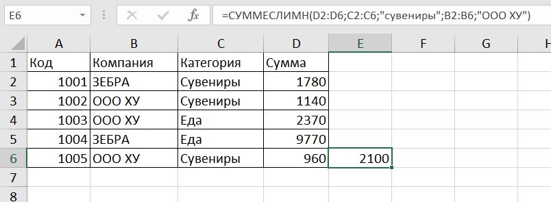
=СУММЕСЛИМН (D2: D6; C2: C6;”сувениры”; B2: B6;”ООО ХУ»)
D2: D6 — диапазон, где суммируются числа;
C2: C6 — диапазон ячеек для категории; сувениры — обязательное условие 1, то есть числа другой категории не учитываются;
B2: B6 — дополнительный диапазон;
ООО XY — условие 2, то есть числа другой компании не учитываются.
Дополнительных диапазонов и условий может быть до 127 штук.
СЧЕТ
=СЧЁТ (значение1; [значение2];…)Формула считает количество выбранных ячеек с числами в заданном диапазоне. Ячейки с датами тоже учитываются.
=СЧЁТ (значение1; [значение2];…)
Формула считает количество выбранных ячеек с числами в заданном диапазоне. Ячейки с датами тоже учитываются.
СЧЕТЕСЛИ и СЧЕТЕСЛИМН
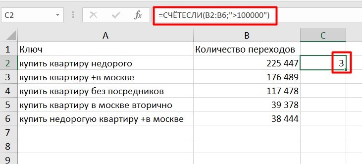
=СЧЕТЕСЛИ (диапазон; критерий)
Функция определяет количество заполненных клеточек, которые подходят под конкретные условия в рамках указанного диапазона.
Например:
=СЧЁТЕСЛИМН (диапазон_условия1; условие1 [диапазон_условия2; условие2];…)
Эта формула позволяет использовать одновременно несколько критериев.
ЕСЛИОШИБКА
=ЕСЛИОШИБКА (значение; значение_если_ошибка)
Функция проверяет ошибочность значения или вычисления, а если ошибка отсутствует, возвращает его.
ДНИ
=ДНИ (конечная дата; начальная дата)
Функция показывает количество дней между двумя датами. В формуле указывают сначала конечную дату, а затем начальную.
КОРРЕЛ
=КОРРЕЛ (диапазон1; диапазон2)
Определяет статистическую взаимосвязь между разными данными: курсами валют, расходами и прибылью и т.д. Мах значение — +1, min — −1.
ВПР
=ВПР (искомое_значение; таблица; номер_столбца;[интервальный_просмотр])
Находит данные в таблице и диапазоне.
Например:
=ВПР (В1; С1: С26;2)
В1 — значение, которое ищем.
С1: Е26— диапазон, в котором ведется поиск.
2 — номер столбца для поиска.
ЛЕВСИМВ
=ЛЕВСИМВ (текст;[число_знаков])
Позволяет выделить нужное количество символов. Например, она поможет определить, поместится ли строка в лимитированное количество знаков или нет.
ПСТР
=ПСТР (текст; начальная_позиция; число_знаков)
Помогает достать определенное число знаков с текста. Например, можно убрать лишние слова в ячейках.
ПРОПИСН
=ПРОПИСН (текст)
Простая функция, которая делает все литеры в заданной строке прописными.
СТРОЧН
Функция, обратная предыдущей. Она делает все литеры строчными.
ПОИСКПОЗ
=ПОИСКПОЗ (искомое_значение; просматриваемый_массив; тип_сопоставления)
Дает возможность найти нужный элемент в заданном блоке ячеек и указывает его позицию.
ДЛСТР
=ДЛСТР (текст)
Данная функция определяет длину заданной строки. Пример использования — определение оптимальной длины описания статьи.
СЦЕПИТЬ
=СЦЕПИТЬ (текст1; текст2; текст3)
Позволяет сделать несколько строчек из одной и записать до 255 элементов (8192 символа).
ПРОПНАЧ
=ПРОПНАЧ (текст)
Позволяет поменять местами прописные и строчные символы.
ПЕЧСИМВ
=ПЕЧСИМВ (текст)
Можно убрать все невидимые знаки из текста.
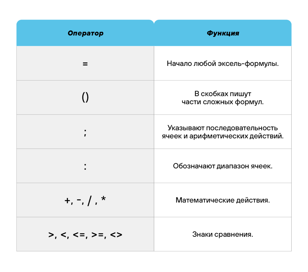
Использование операторов
Операторы в Excel указывают, какие конкретно операции нужно выполнить над элементами формулы. В вычислениях всегда соблюдается математический порядок:
-
скобки;
-
экспоненты;
-
умножение и деление;
-
сложение и вычитание.
Арифметические
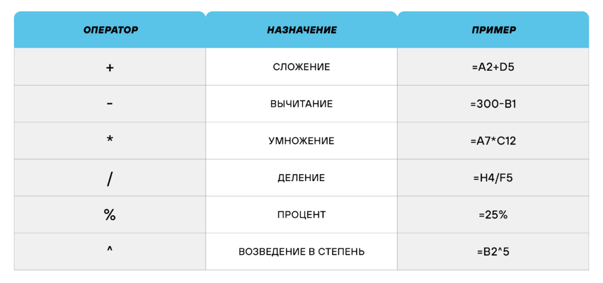
Операторы сравнения
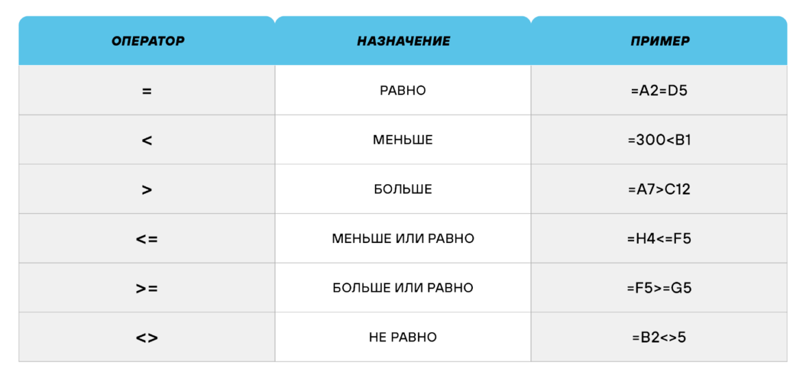
Оператор объединения текста
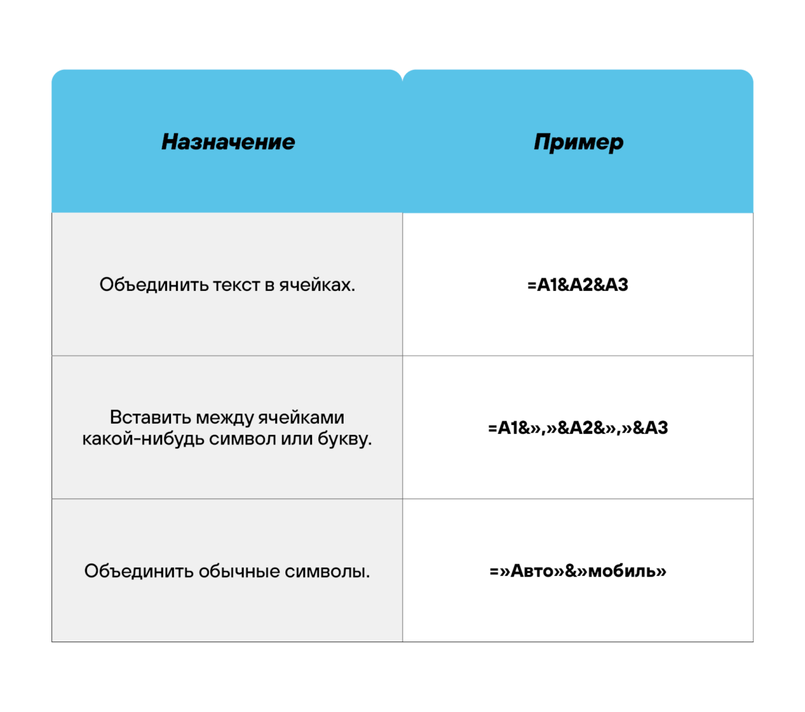
Операторы ссылок
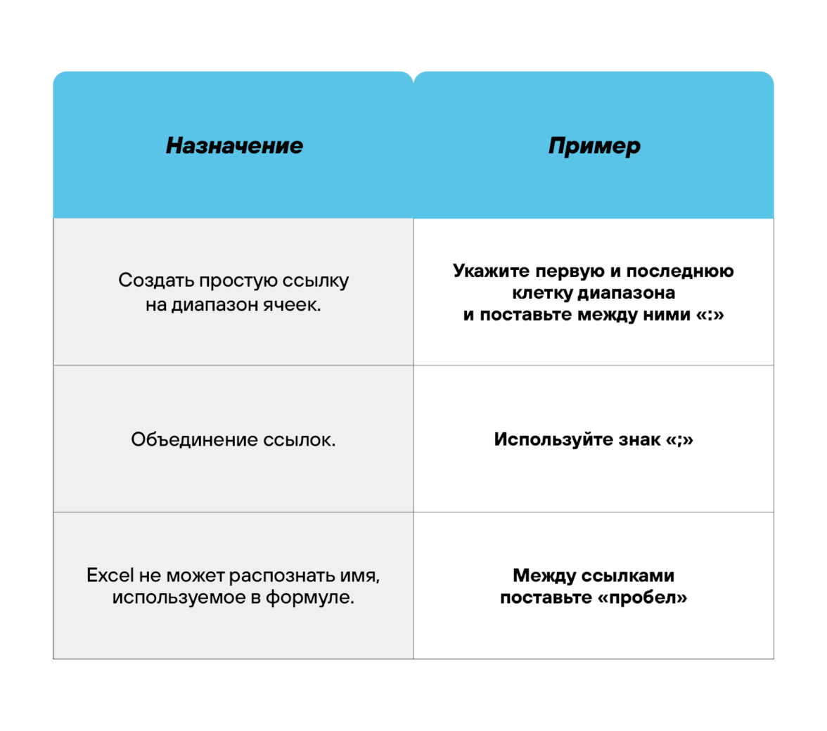
Использование ссылок
Начинающие пользователи обычно работают только с простыми ссылками, но мы расскажем обо всех форматах, даже продвинутых.
Простые ссылки A1
Они используются чаще всего. Буква обозначает столбец, цифра — строку.
Примеры:
-
диапазон ячеек в столбце С с 1 по 23 строку — «С1: С23»;
-
диапазон ячеек в строке 6 с B до Е– «B6: Е6»;
-
все ячейки в строке 11 — «11:11»;
-
все ячейки в столбцах от А до М — «А: М».
Ссылки на другой лист
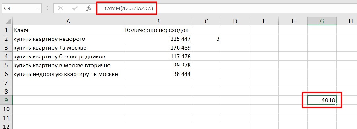
Если необходимы данные с других листов, используется формула: =СУММ (Лист2! A5: C5)
Выглядит это так:
Абсолютные и относительные ссылки
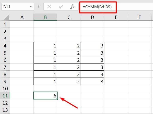
Относительные ссылки
Рассмотрим, как они работают на примере: Напишем формулу для расчета суммы первой колонки. =СУММ (B4: B9)
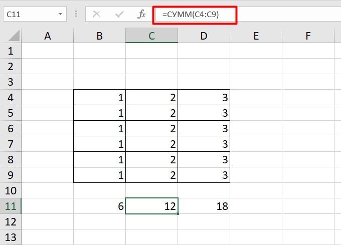
Нажимаем на Ctrl+C. Чтобы перенести формулу на соседнюю клетку, переходим туда и жмем на Ctrl+V. Или можно просто протянуть ячейку с формулой, как мы описывали выше.
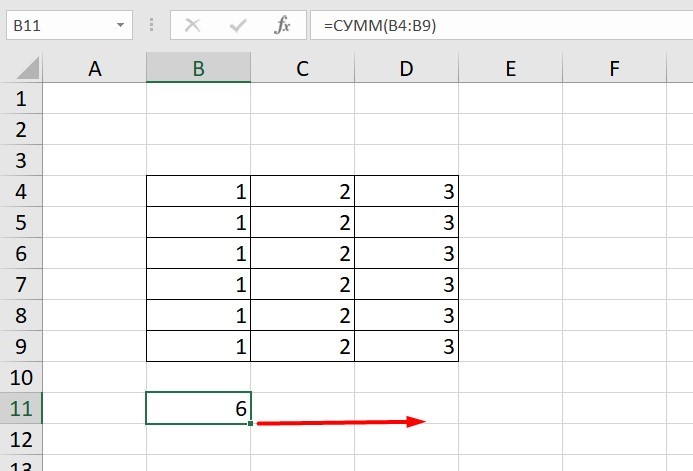
Индекс таблицы изменится автоматически и новые формулы будут выглядеть так:
Абсолютные ссылки
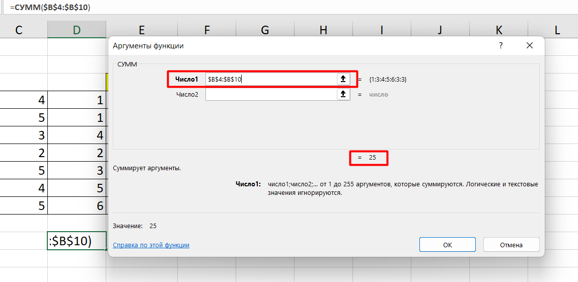
Чтобы при переносе формул ссылки сохранялись неизменными, требуются абсолютные адреса. Их пишут в формате «$B$2».
Например, есть поставить знак доллара в предыдущую формулу, мы получим: =СУММ ($B$4:$B$9)
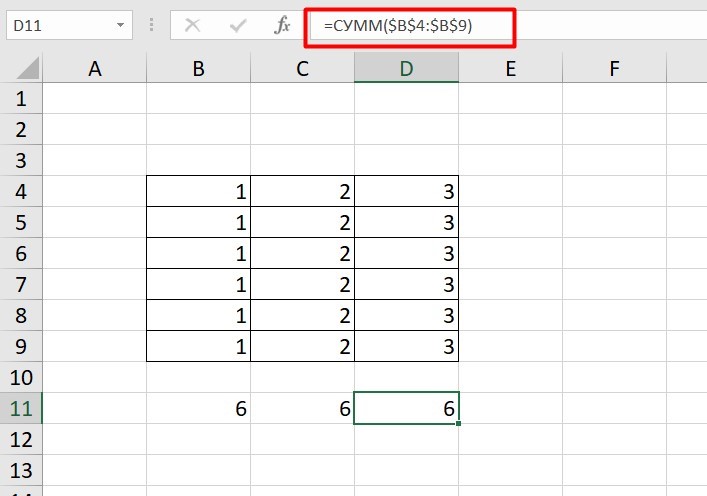
Как видите, никаких изменений не произошло.
Смешанные ссылки
Они используются, когда требуется зафиксировать только столбец или строку:
-
$А1– сохраняются столбцы;
-
А$1 — сохраняются строки.
Смешанные ссылки удобны, когда приходится работать с одной постоянной строкой данных и менять значения в столбцах. Или, когда нужно рассчитать результат в ячейках, не расположенных вдоль линии.
Трёхмерные ссылки
Это те, где указывается диапазон листов.
Формула выглядит примерно так: =СУММ (Лист1: Лист5! A6)
То есть будут суммироваться все ячейки А6 на всех листах с первого по пятый.
Ссылки формата R1C1
Номер здесь задается как по строкам, так и по столбцам.
Например:
-
R9C9 — абсолютная ссылка на клетку, которая расположена на девятой строке девятого столбца;
-
R[-2] — ссылка на строчку, расположенную выше на 2 строки;
-
R[-3]C — ссылка на клетку, которая расположена на 3 ячейки выше;
-
R[4]C[4] — ссылка на ячейку, которая распложена на 4 клетки правее и 4 строки ниже.
Использование имён
Функционал Excel позволяет давать собственные уникальные имена ячейкам, таблицам, константам, выражениям, даже диапазонам ячеек. Эти имена можно использовать для совершения любых арифметических действий, расчета налогов, процентов по кредиту, составления сметы и табелей, расчётов зарплаты, скидок, рабочего стажа и т.д.
Все, что нужно сделать — заранее дать имя ячейкам, с которыми планируете работать. В противном случае программа Эксель ничего не будет о них знать.
Как присвоить имя:
-
Выделите нужную ячейку/столбец.
-
Правой кнопкой мышки вызовите меню и перейдите в закладку «Присвоить имя».
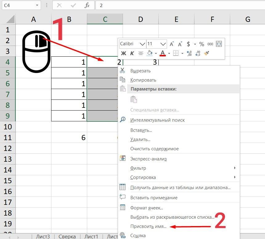
-
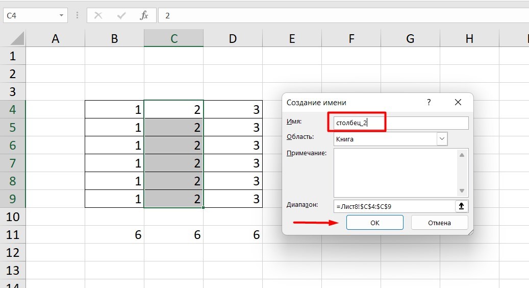
Напишите желаемое имя, которое должно быть уникальным и не повторяться в одной книге.
-
Сохраните, нажав Ок.
Использование функций
Чтобы вставить необходимую функцию в эксель-таблицах, можно использовать три способа: через панель инструментов, с помощью опции Вставки и вручную. Рассмотрим подробно каждый способ.
Ручной ввод
Этот способ подойдет тем, кто хорошо разбирается в теме и умеет создавать формулы прямо в строке. Для начинающих пользователей и новичков такой вариант покажется слишком сложным, поскольку надо все делать руками.
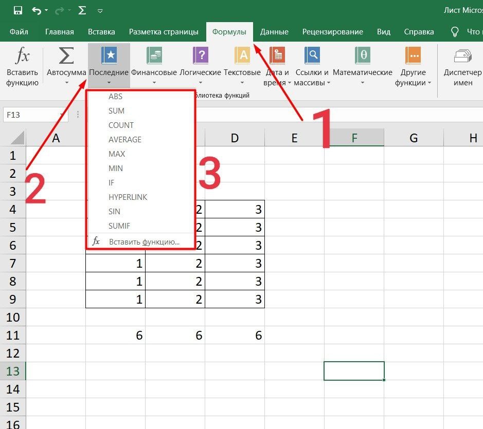
Панель инструментов
Это более упрощенный способ. Достаточно перейти в закладку «Формулы», выбрать подходящую библиотеку — Логические, Финансовые, Текстовые и др. (в закладке «Последние» будут наиболее востребованные формулы). Остается только выбрать из перечня нужную функцию и расставить аргументы.
Мастер подстановки
Кликните по любой ячейке в таблице. Нажмите на иконку «Fx», после чего откроется «Вставка функций».
Выберите из перечня нужную категорию формул, а затем кликните по функции, которую хотите применить и задайте необходимые для расчетов аргументы.
Вставка функции в формулу с помощью мастера
Рассмотрим эту опцию на примере:
-
Вызовите окошко «Вставка функции», как описывалось выше.
-
В перечне доступных функций выберите «Если».
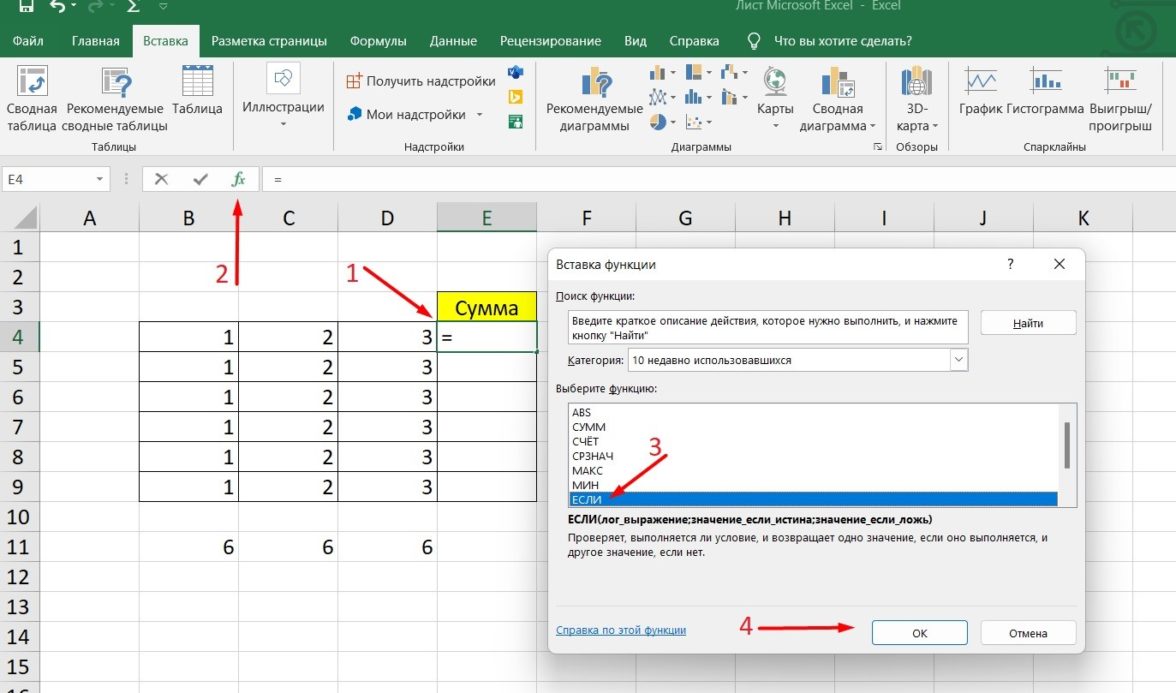
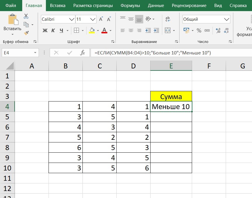
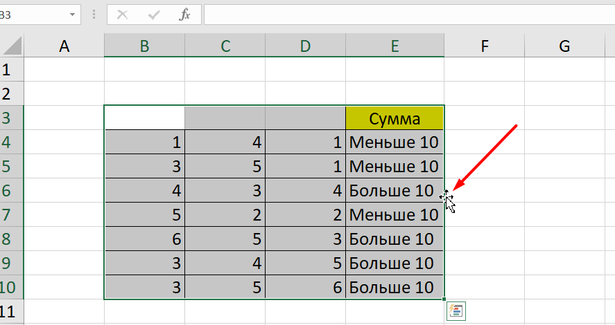
Теперь составим выражение, чтобы проверить, будет ли сумма трех ячеек больше 10. При этом Правда — «Больше 10», а Ложь — «Меньше 10».
=ЕСЛИ (СУММ (B3: D3)>10;”Больше 10″;»Меньше 10″)
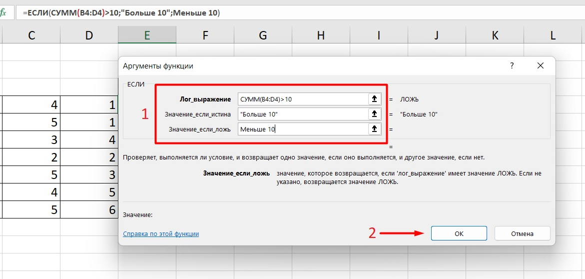
Программа посчитала, что сумма ячеек меньше 10 и выдала нам результат:
Чтобы получить значение в следующих ячейках столбца, нужно растянуть формулу (за правый нижний уголок). Получится следующее:
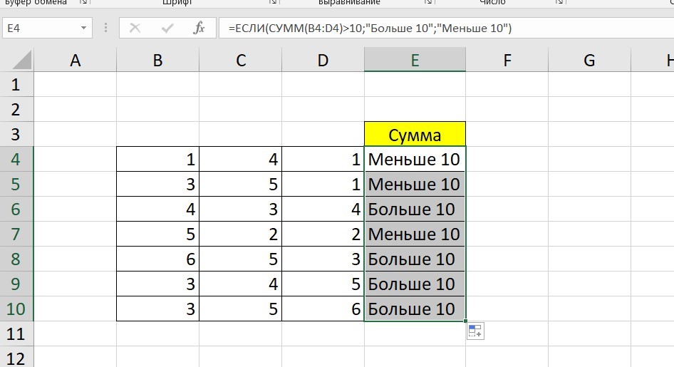
Мы использовали относительные ссылки, поэтому программа пересчитала выражение для всех строк корректно. Если бы нам нужно было зафиксировать адреса в аргументах, тогда мы бы применяли абсолютные ссылки, о которых писали выше.
Редактирование функций с помощью мастера
Чтобы отредактировать функцию, можно использовать два способа:
-
Строка формул. Для этого требуется перейти в специальное поле и вручную ввести необходимые изменения.
-
Специальный мастер. Нажмите на иконку «Fx» и в появившемся окошке измените нужные вам аргументы. И тут же, кстати, сможете узнать результат после редактирования.
Операции с формулами
С формулами можно совершать много операций — копировать, вставлять, перемещать. Как это делать правильно, расскажем ниже.
Копирование/вставка формулы
Чтобы скопировать формулу из одной ячейки в другую, не нужно изобретать велосипед — просто нажмите старую-добрую комбинацию (копировать), а затем кликните по новой ячейке и нажмите (вставить).
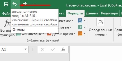
Отмена операций
Здесь вам в помощь стандартная кнопка «Отменить» на панели инструментов. Нажмите на стрелочку возле нее и выберите из контекстного меню те действия. которые хотите отменить.
Повторение действий
Если вы выполнили команду «Отменить», программа сразу активизирует функцию «Вернуть» (возле стрелочки отмены на панели). То есть нажав на нее, вы повторите только что отмененную вами операцию.
Стандартное перетаскивание
Выделенные ячейки переносятся с помощью указателя мышки в другое место листа. Делается это так:
-
Выделите фрагмент ячеек, которые нужно переместить.
-
Поместите указатель мыши над одну из границ фрагмента.
-
Когда указатель мыши станет крестиком с 4-мя стрелками, можете перетаскивать фрагмент в другое место.
Копирование путем перетаскивания
Если вам нужно скопировать выделенный массив ячеек в другое место рабочего листа с сохранением данных, делайте так:
-
Выделите диапазон ячеек, которые нужно скопировать.
-
Зажмите клавишу и поместите указатель мыши на границу выбранного диапазона.
-
Он станет похожим на крестик +. Это говорит о том, что будет выполняться копирование, а не перетаскивание.
-
Перетащите фрагмент в нужное место и отпустите мышку. Excel задаст вопрос — хотите вы заменить содержимое ячеек. Выберите «Отмена» или ОК.
Особенности вставки при перетаскивании
Если содержимое ячеек перемещается в другое место, оно полностью замещает собой существовавшие ранее записи. Если вы не хотите замещать прежние данные, удерживайте клавишу в процессе перетаскивания и копирования.
Автозаполнение формулами
Если необходимо скопировать одну формулу в массив соседних ячеек и выполнить массовые вычисления, используется функция автозаполнения.
Чтобы выполнить автозаполнение формулами, нужно вызвать специальный маркер заполнения. Для этого наведите курсор на нижний правый угол, чтобы появился черный крестик. Это и есть маркер заполнения. Его нужно зажать левой кнопкой мыши и протянуть вдоль всех ячеек, в которых вы хотите получить результат вычислений.
Как в формуле указать постоянную ячейку
Когда вам нужно протянуть формулу таким образом, чтобы ссылка на ячейку оставалась неизменной, делайте следующее:
-
Кликните на клетку, где находится формула.
-
Наведите курсор в нужную вам ячейку и нажмите F4.
-
В формуле аргумент с номером ячейки станет выглядеть так: $A$1 (абсолютная ссылка).
-
Когда вы протяните формулу, ссылка на ячейку $A$1 останется фиксированной и не будет меняться.
Как поставить «плюс», «равно» без формулы
Когда нужно указать отрицательное значение, поставить = или написать температуру воздуха, например, +22 °С, делайте так:
-
Кликаете правой кнопкой по ячейке и выбираете «Формат ячеек».
-
Отмечаете «Текстовый».
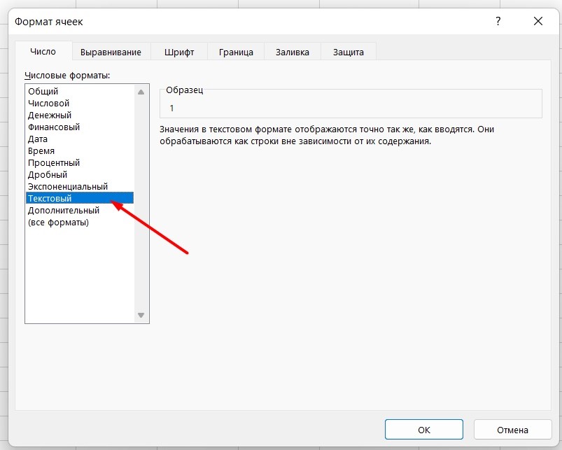
Теперь можно ставить = или +, а затем нужное число.
Самые распространенные ошибки при составлении формул в редакторе Excel
Новички, которые работают в редакторе Эксель совсем недавно, часто совершают элементарные ошибки. Поэтому рекомендуем ознакомиться с перечнем наиболее распространенных, чтобы больше не ошибаться.
-
Слишком много вложений в выражении. Лимит 64 штуки.
-
Пути к внешним книгам указаны не полностью. Проверяйте адреса более тщательно.
-
Неверно расставленные скобочки. В редакторе они обозначены разными цветами для удобства.
-
Указывая имена книг и листов, пользователи забывают брать их в кавычки.
-
Числа в неверном формате. Например, символ $ в Эксель — это не знак доллара, а формат абсолютных ссылок.
-
Неправильно введенные диапазоны ячеек. Не забывайте ставить «:».
Коды ошибок при работе с формулами
Если вы сделаете ошибку в записи формулы, программа укажет на нее специальным кодом. Вот самые распространенные:
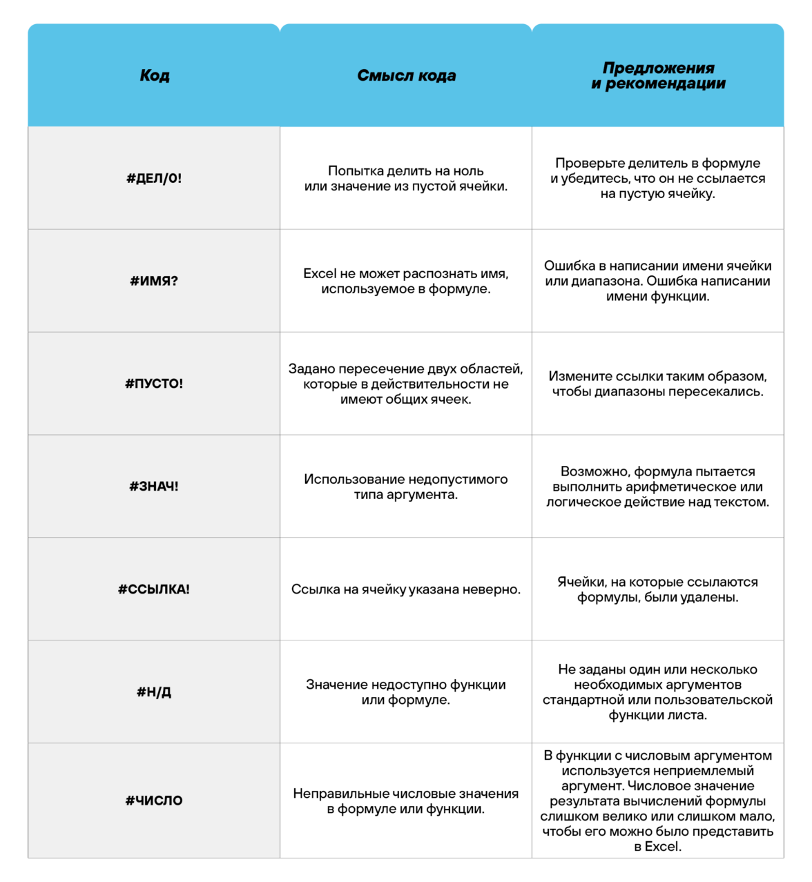
Отличие в версиях MS Excel
Всё, что написано в этом гайде, касается более современных версий программы 2007, 2010, 2013 и 2016 года. Устаревший Эксель заметно уступает в функционале и количестве доступных инструментов. Например, функция СЦЕП появилась только в 2016 году.
Во всем остальном старые и новые версии Excel не отличаются — операции и расчеты проводятся по одинаковым алгоритмам.
Заключение
Мы написали этот гайд, чтобы вам было легче освоить Excel. Доступным языком рассказали о формулах и о тех операциях, которые можно с ними проводить.
Надеемся, наша шпаргалка станет полезной для вас. Не забудьте сохранить ее в закладки и поделиться с коллегами.
List of Top 10 Advanced Excel Formulas & Functions
You can download this Advanced Excel Formulas Template here – Advanced Excel Formulas Template
Table of contents
- List of Top 10 Advanced Excel Formulas & Functions
- #1 – VLOOKUP Formula in Excel
- #2 – INDEX Formula in Excel
- #3 – MATCH Formula in Excel
- #4 – IF AND Formula in Excel
- #5 – IF OR Formula in Excel
- #6 – SUMIF Formula in Excel
- #7 – CONCATENATE Formula in Excel
- #8 – LEFT, MID, and RIGHT Formula in Excel
- #9 – OFFSET Formula in Excel
- #10 – TRIM Formula in Excel
- Recommended Articles
#1 – VLOOKUP Formula in Excel
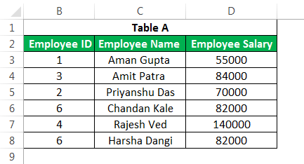
This advanced Excel function is one of the most used formulae in Excel. It is mainly due to the simplicity of this formula and its application in looking up a certain value from other tables, which has one standard variable across these tables. For example, suppose you have two tables detailing a company’s employee salary and name, with “Employee ID” being a primary column. You want to get the salary from Table B in Table A.
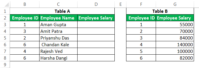
You can use VLOOKUPThe VLOOKUP excel function searches for a particular value and returns a corresponding match based on a unique identifier. A unique identifier is uniquely associated with all the records of the database. For instance, employee ID, student roll number, customer contact number, seller email address, etc., are unique identifiers.
read more as below.

It will result in the table below when we apply this advanced Excel formula in other cells of the “Employee Salary” column.

Drag the formula to the rest of the cells.
There are three major delimitations of VLOOKUP:
- You cannot have a primary column on the right of the column for which you want to populate the value from another table. The “Employee Salary” column cannot be before the “Employee ID.”
- In the duplicated values in the primary column in Table B, the first value will get populated in the cell.
- If you insert a new column in the database (e.g., insert a new column before “Employee Salary” in Table B), the output of the formula could be different based on the position that you have mentioned in the formula (in the above case, the result would be blank).
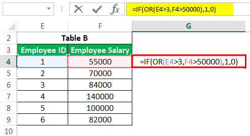
#2 – INDEX Formula in Excel
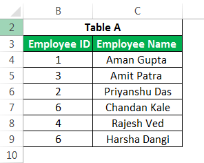
This advanced Excel formula is used to get the value of a cell in a given table by specifying the number of rows, columns, or both. E.g., to get an employee’s name at the 5th observation. Below is the data.
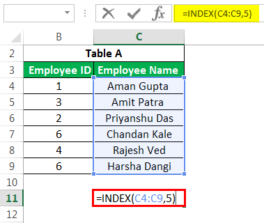
We can use the advanced Excel formula below:
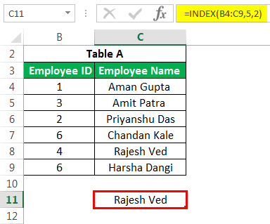
We can use the same INDEX formula in getting values along the row. So, for example, when using both row and column numbers, the syntax would look like this:

The above formula would return as “Rajesh Ved.”
Note: If you insert another row into the 5th row, the formula will return as “Chandan Kale.” Hence, the output would depend on any changes in the data table over time.

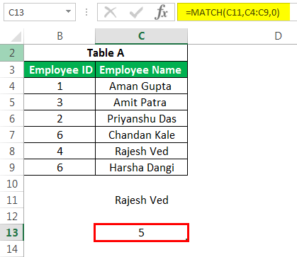
#3 – MATCH Formula in Excel
This Excel advanced formula returns the row or column number when a specific string or number is in the given range. In the below example, we are trying to find “Rajesh Ved” in the “Employee Name” column.
The formula would be as given below:

The MATCH functionThe MATCH function looks for a specific value and returns its relative position in a given range of cells. The output is the first position found for the given value. Being a lookup and reference function, it works for both an exact and approximate match. For example, if the range A11:A15 consists of the numbers 2, 9, 8, 14, 32, the formula “MATCH(8,A11:A15,0)” returns 3. This is because the number 8 is at the third position.
read more would return 5 as the value.
The 3rd argument is used for the exact match. You can also use +1 and -1 based on your requirements.
Note: One can combine INDEX and MATCH to overcome the limitation of VLOOKUP.
#4 – IF AND Formula in Excel
There are many instances when one needs to create flags based on some constraints. We all are familiar with the basic syntax of IF. We use this advanced excel IF functionIF function in Excel evaluates whether a given condition is met and returns a value depending on whether the result is “true” or “false”. It is a conditional function of Excel, which returns the result based on the fulfillment or non-fulfillment of the given criteria.
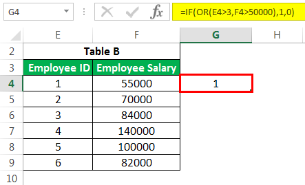
read more to create a new field based on some existing field constraints. But what if we need to consider multiple columns while creating a flag? E.g., in the below case, we want to flag all the employees whose salary is greater than 50,000. But “Employee ID” is greater than 3.
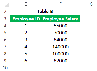
We would use the IF AND formula in such cases. Please find below the screenshot for the same.
It would return the result as 0.

We can have many conditions or constraints to create a flag based on multiple columns using AND.
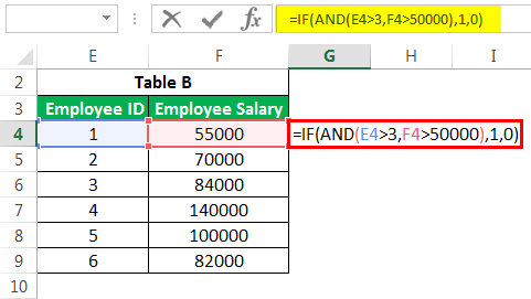
#5 – IF OR Formula in Excel
Similarly, we can use the OR function in ExcelThe OR function in Excel is used to test various conditions, allowing you to compare two values or statements in Excel. If at least one of the arguments or conditions evaluates to TRUE, it will return TRUE. Similarly, if all of the arguments or conditions are FALSE, it will return FASLE.read more instead of AND if we need to satisfy one of the many conditions.
If any condition is satisfied in the above cases, we will have the cell populated as 1, else 0. We can substitute 1 or 0 with some substrings with double quotes (“”).
#6 – SUMIF Formula in Excel
In some analyses, you might need to filter observations when applying the sum or count function. In such cases, this advanced Excel SUMIF function in excelThe SUMIF Excel function calculates the sum of a range of cells based on given criteria. The criteria can include dates, numbers, and text. For example, the formula “=SUMIF(B1:B5, “<=12”)” adds the values in the cell range B1:B5, which are less than or equal to 12.
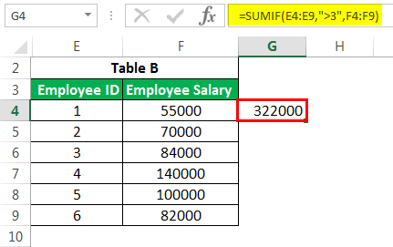
read more is at our rescue. It filters all the observations based on certain conditions in this advanced excel formula and sums up them. E.g., What if we want to know the sum of salaries of only those employees with employee IDs greater than 3?
By applying the SUMIFS formulaSUMIFS is an enhanced version of the SUMIF formula in Excel that enables you to sum any range of data by matching several criteria. read more:
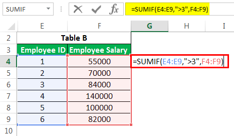
The formula returns the results as 322000.
We can also count the number of employees in the organization having an employee ID greater than 3 using COUNTIF instead of SUMIF.
#7 – CONCATENATE Formula in Excel
This Excel advanced function is one of the formulas used with multiple variants. This advanced Excel formula helps us join several text strings into one text string. For example, if we want to show “Employee ID” and “Employee Name” in a single column.
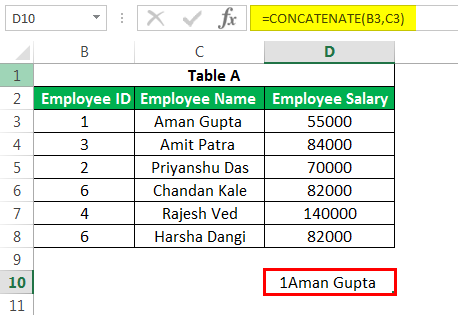
We can use this CONCATENATE formula here.
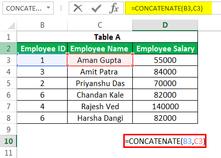
The above formula will result in “1Aman Gupta”.
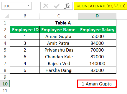
We can have one more variant by putting a single hyphen between ID and NAME. E.g., CONCATENATE(B3,”-“,C3) will result in “1-Aman Gupta”. We can also use this in VLOOKUP when LOOKUP in ExcelThe LOOKUP excel function searches a value in a range (single row or single column) and returns a corresponding match from the same position of another range (single row or single column). The corresponding match is a piece of information associated with the value being searched.
read more value is a mixture of more than one variable.
#8 – LEFT, MID, and RIGHT Formula in Excel
We can use this advanced Excel formula to extract a specific substring from a given string. One could use it based on our requirements. E.g., If we want to remove the first 5 characters from “Employee Name,” we can use the LEFT formula in ExcelThe left function returns the number of characters from the start of the string. For example, if we use this function as =LEFT ( «ANAND»,2), the result will be AN.read more with the column name and second parameter as 5.
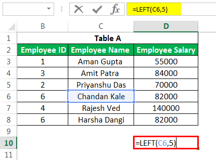
The output is given below:

The application of the RIGHT formula in ExcelRight function is a text function which gives the number of characters from the end from the string which is from right to left. For example, if we use this function as =RIGHT ( “ANAND”,2) this will give us ND as the result.read more is also the same. It is just that we would be looking at the character from the right of the string. However, in the case of a MID function in excelThe mid function in Excel is a text function that finds strings and returns them from any mid-part of the spreadsheet. read more, we must give the required text string’s starting position and the string’s length.
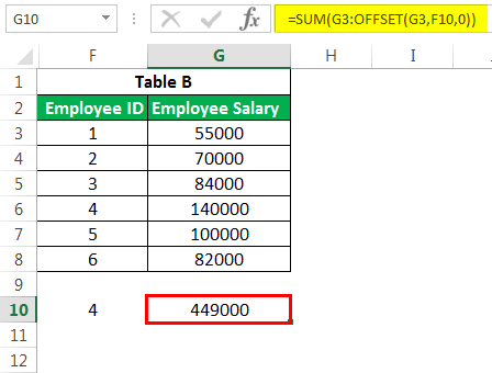
#9 – OFFSET Formula in Excel
This advanced Excel function, combined with SUM or AVERAGE, could give a dynamic touch to the calculations. It is best used when we insert continuous rows into an existing database. OFFSET ExcelThe OFFSET function in excel returns the value of a cell or a range (of adjacent cells) which is a particular number of rows and columns from the reference point. read more provides a range where we need to mention reference cells, number of rows, and columns. E.g., If we want to calculate the average of the first 5 employees in the company where we have the salary of employees sorted by employee ID, we can do the following. The calculation below will always give us a salary.

- It will give us the sum of salaries of the first 5 employees.
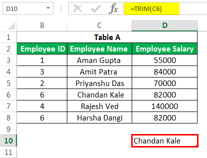
#10 – TRIM Formula in Excel
This advanced Excel formula is used to clean up the unimportant spaces in the text. E.g., if we want to remove spaces at the beginning of some name, we can use it by using the TRIM function in ExcelThe Trim function in Excel does exactly what its name implies: it trims some part of any string. The function of this formula is to remove any space in a given string. It does not remove a single space between two words, but it does remove any other unwanted spaces.read more as below:
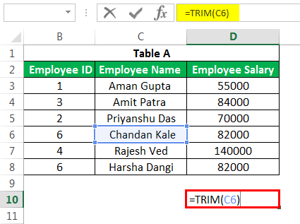
The resultant output would be “Chandan Kale” without space before Chandan.
Recommended Articles
This article is a guide to Advanced Formulas in Excel. We discuss the top 10 Advanced Excel formulas and Advanced Excel functions with a downloadable template. You may learn more about Excel from the following articles: –
- Basic Excel Formulas
- VBA MID Function
- Match in Excel
- VLookup with IF
You may be familiar with Microsoft Excel. This application made by Microsoft Corporation is the application with the most users in the world in 140+ countries. This application has a myriad of Excel formulas that can accurately present numbers and data.
The primary function of Microsoft Excel is calculation, which is why it has been used by many users, both students and office workers. Despite other spreadsheet programs (competitors), Excel maintained its dominance and even became an industry standard.
Apparently, Excel seems too good to be true. All you have to do is enter an Excel formula, and almost everything you need to do manually can be done automatically. Use the best accounting software to do the cash flow forecast appropriately and analyze financial statements more optimally.
If you need to combine two sheets with the same data, Excel can do this. Do you need help with mathematics? Excel can do this. Are you using data from multiple cells? Excel can do this too.
In this article, you will understand the function of Excel in different professional fields. Then you’ll understand what formulas you need to know. Later, you will be able to apply automatic calculations to be used according to your needs.
Table Of Content
- The Uses of Excel in Professional Fields
- Complete Excel Formulas with Their Functions
- Conclusion
Also Read: 5 Common Bookkeeping Mistakes on Small Businesses
The Uses of Excel in Professional Fields
Many job openings require candidates to master Excel. Not surprisingly, excel is needed by a wide variety of fields of work that require data collection.
To that end, we will present the following professions, which can benefit from the use of Excel, among others:
Accountancy
It is widespread for accountants to be able to use Excel. The field of accounting benefits from using Microsoft Excel in several ways, including making it easier to calculate corporate profit and loss, identify large profits over a period, calculate employee salaries, and more.
An accountant can facilitate his work by using the accounting system as a tool he worked. The system can provide convenience in managing the company’s financial circulation and calculating it optimally and accurately.
Also Read: Salary Slip: Understanding, Benefits, Format, Example
Mathematical calculations
The next advantage of using Microsoft Excel is mathematical calculations. Use calculations to find data from numbers, subtractions, multiplications, and divisions, as well as various other variations such as calculating the slope.
Data processing
In data management, there are helpful excel formulas, including managing statistical databases, calculating data, searching for median values, and averages, and searching for the maximum and minimum values of data sets.
Graphic creation
Excel allows you to create graphics. Such as graphing population development data for one year, the graph of student library visits for one year, the student graduation graph for six years, the graph of student number development for three years, and others.
Table operations
The last application is to be able to operate the table. With a total of 1,084,576 rows and 16,384 columns in Microsoft Excel, it will make it easier for you to enter data that requires a large number of columns and rows.
Complete Excel Formulas with Their Functions
In addition to the functionality and use of Microsoft Excel mentioned earlier, operating this Excel program requires Excel formulas. Each formula has a different function that you can use for a specific need.
Here are the Excel formulas you need to know, among others:
| Formulas | Functional Description |
| SUM | Summing |
| AVERAGE | Looking for Average Values |
| AND | Finding Value by comparison and |
| NOT | Finding Value with Exceptions |
| OR | Finding Value by Comparison or |
| SINGLE IF | Looking for Values If Conditions ARE RIGHT/WRONG |
| MULTI IF | Finding Values If Conditions ARE RIGHT/WRONG With Many Comparisons |
| AREAS | View The Number of Areas (Range or Cells) |
| CHOOSE | View Selection Results Based on Index Numbers |
| HLOOKUP | Search for Data from a table organized in a horizontal format |
| VLOOKUP | Search for Data from a table arranged in an upright format |
| MATCH | Displays the position of a specific cell address |
| COUNTIF | Counting the Number of Cells in a Range with specific criteria |
| COUNTA | Counting the Number of Filled Cells |
| CEILING | Round the number up |
| FLOOR | Rounds numbers down |
| DAY | Looking for The Value of the Day |
| MONTH | Searching for the Value of the Moon |
| YEAR | Looking for Year Value |
| DATE | Get a Date Value |
| LOWER | Change text letters to lowercase |
| UPPER | Change Text Letters to UpperCase |
| PROPER | Change the Initial Character of the Text To UpperCase |
For more information about how to use the excel function formulas mentioned above, here is a detailed description, along with examples:
SUM
This Excel summation formula has the primary function of summing numbers in specific cells. However, it is also often used to complete a job or task quickly.
To use SUM, first create a summation table and enter the summation formula below. For example, =SUM(G8:H8), or as shown in the image below:
Then, if the SUM formula has been entered, press enters to specify the amount. As shown in the picture below:
AVERAGE
The primary function of the AVERAGE formula or the average formula in Excel is to find the average value of a variable. The trick is to create a table for grades and then enter the AVERAGE formula to determine the student’s grade point average. For example, =AVERAGE(D2:F2), as in the following image:
If you enter the AVERAGE formula, press enters to see the result, shown in the image below.
AND
The AND formula function generates a TRUE value if all previously tested arguments are correct or can return a FALSE value if all arguments or answers are incorrect.
To determine TRUE or FALSE, you must create a table and enter THE FORMULA AND. For example, =AND(G7>I7).
This technique is usually used to help fill out questionnaires or answer question columns to speed up the value-setting process.
NOT
The NOT formula has the opposite function of the AND formula because it produces TRUE if the condition tested is FALSE and FALSE if the condition tested is TRUE.
The first step is to create a table and enter the FORMULA NOT to find out the results. For example, as shown in the diagram below, =NOT(G7>J7).
OR
The OR is the following excel formula that will produce TRUE data if some given argument is correct. If all of the arguments presented are incorrect, the answer is FALSE.
A student’s average test score result is an example of how OR can use it in Excel. If it is less than 70, he must repeat the course; if it is greater than 70, the student graduates.
SINGLE IF
The IF function is to return a value that, when examined, is TRUE and another value that is visible as FALSE.
Not much different from the technique of using formulas in OR. It just seems more straightforward.
For example, when a student’s average grade is less than 75, that student does not graduate, and vice versa. How to create an IF formula is =IF(J8<75;” NOT GRADUATING”;” PASS”). To be clear, take a look at the following image:
After entering the formula, press enters, and the result will match what you ordered.
MULTI IF
This formula is a further lesson from SINGLE IF, but if SINGLE IF only uses only one condition with two options, The MULTI IF uses two terms and three options.
A Double/Multi FORMULA is a type of logic-IF formula consisting of 2 or more IF in formula writing. If a single IF only needs 1 IF, for example, =IF(B2=>=70;” Graduated”;” Failed”) then Double IF requires more than 1 IF, for example, =IF(B2>=70;” Good”;IF(B2>=50;” Enough”;” Less”)).
So that the full Excel formula will provide Syntax on Double / Multi IF, among others:
=IF(Logical_Test; Value_If_True;IF(Logical_Test; Value_If_True; Value_If_False))
AREAS
You can use the usability of AREAS if you want to calculate the number of areas you want to select. The AREAS formula can use the formula =AREAS(G6:K8).
The result is one area. The results are based on the example in the image of selecting only one range of cells.
CHOOSE
The primary function of a CHOOSE formula is to display selection results based on index numbers or sequences in reference (VALUE) that contain text, numeric, formula, or range names. The image below shows an example of how to write the CHOOSE formula.
Meanwhile, the results of the CHOOSE formula are shown in the image below.
HLOOKUP
The HLOOKUP function displays data from tables arranged horizontally. However, The arrangement of tables or data in the first row should be based on small to large sequences or raising them.
For example, the number 1,2,3,4… Or the letter A-Z. Sort by ascending the menu if you previously typed randomly. Cases like the ones listed below are examples.
=HLOOKUP(Cells that contain packet types; Range cell table details costs; The location of the data column you want to retrieve;0).
VLOOKUP
The primary function of the VLOOKUP formula is almost identical to the HLOOKUP formula; The difference is that the VLOOKUP formula displays data from tables arranged in an upright or vertical format. The requirement is that the first row of the data table is prepared in small to large order or up.
For example 1,2,3,4… Or the letter A-Z. For example 1,2,3,4… Or the letter A-Z. Sort through the Ascending menu if you previously typed randomly.
MATCH
The MATCH function is one of the components of an Excel formula that you can use to perform lookups or reference data searches.
The MATCH function works by finding the relative position of a value in a range or array and generating a number that is the index of the cell’s relative position that contains the value it is looking for.
The use of the Excel MATCH function must follow the syntax rules, namely MATCH(lookup_value, lookup_array, [match_type])
To better understand, understand the image below:
COUNTIF
COUNTIF is a helpful formula for counting the number of cells that have the same criteria. As a result, you no longer have to struggle with data sorting.
Assume you’re doing a survey. You want to know how many civil servants there are out of 20 respondents. As a result, you can use the following formulas:
To get started, all you need to do is enter the range of cells you want to identify into the COUNTIF formula (B2:B21)
Then, enter the cell calculation criteria, namely “PNS” (must be in quotation marks).
This formula produces a result of 7. So, out of 20 respondents, seven were civil servants.
COUNTA
COUNTA has the function of counting the number of cells that contain numbers and the number of cells that contain anything. As a result, you can determine the number of cells that are not empty.
Assume that cells A1 through D1 are words and cells G1 through I1 number. Therefore the use of the formula is =COUNTA(A1:I1)
That results in 7 because the empty cells are only E1 and F1.
CEILING
The CEILING formula can round the number UP at the multiple values of a specific number. The formula is CEILING (CELLS number; Multiples).
Misalnya, CEILING(G9;100). Then the number on Cells G9 will be rounded up with a multiple of 100.
FLOOR
If the previous use of the formula is to round to the nearest integer and above, the FLOOR formula is used to round to the nearest integer. The formula is almost identical to the one for CEILING, but with the addition of FLOOR.
The FLOOR formula is FLOOR (Number cell; Multiples).
DAY
The DAY formula is used to find the date type data’s day (in the numbers 1-31). Consider the DAY function (column B). The date data in column A will be extracted and converted into numbers 1-31, following the explanation through the image:
After entering the formula =DAY(NUMBER), press enters and see the results below:
MONTH
Almost similar to the DAY formula, the use of the MONTH formula to search for months (in numbers 1-12) from date type data. For example, the use of the MONTH function (column K) of a column I date data, after extracting it, produces the numbers 1-12 as in the figure below:
YEAR
Meanwhile, there is a YEAR formula. The way you use this formula is similar to the way the previous two formulas were. The use of the YEAR formula takes years (in the range of 1900-9999) from date-type data.
DATE
The DATE formula has a function that allows you to get date data types by entering years, months, and days. The DATE function is the opposite of the DAY, MONTH, and YEAR functions, which describe month and year-type data from their respective dates.
Year, month, and day data in the form of numbers combined with the DATE function generate data with data types, as shown in the figure below. Date formula writing image, namely:
LOWER
The lower formula function converts all uppercase letters in the text to lowercase. To use the formula, type the LOWER command, and texts will convert the desired writing to lowercase.
For example, when implementing the LOWER formula with the formula =LOWER (Don’t Forget to Use HashMicro Software), the result is “don’t forget to use has micro software.”
UPPER
In addition to lower formulas, Microsoft Excel includes upper formulas. The use of UPPER is to convert all text containing lowercase letters into uppercase, the opposite of the LOWER function.
For example, if you type UPPER (hashmicro), your writing will be entirely in capital letters.
PROPER
Sometimes you forget to write sentences in all lowercase letters and no capital letters. So with the PROPER formula, you can capitalize on the first character in each word while keeping the rest. The formula is APPROPRIATE (text).
Conclusion
Although understanding Excel entirely takes time, you will be familiar with all the correct formulas and applications.
In a company, the use of Excel is overwhelming, especially in presenting data, statistics, and company finances such as salaries. The digital world is bringing corporate transformation to provide information and payroll more easily with automated systems. You can use HashMicro accounting software as a tool to calculate financial circulation optimally and accurately.
Moreover, HashMicro has a system that helps with all your human resource and employee administration tasks. With HashMicro’s HRM Software, calculates salaries, and manages leave and attendance lists, reimbursement processes, timesheets, and other operational activities in just seconds.
Produce reports accurately and comprehensively like thousands of large companies that have joined HashMicro. To check out more, click here.
Эти простые, но полезные функции могут пригодиться для самых разных задач.

Чтобы применить любую из перечисленных функций, поставьте знак равенства в ячейке, в которой вы хотите видеть результат. Затем введите название формулы (например, МИН или МАКС), откройте круглые скобки и добавьте необходимые аргументы. Excel подскажет синтаксис, чтобы вы не допустили ошибку.
Аргументами называют данные, с которыми работает функция. Чтобы добавить их, нужно выделить соответствующие ячейки или ввести необходимые значения в скобках вручную.
Есть и альтернативный способ указать аргументы. Если после названия функции добавить пустые скобки и нажать на кнопку «Вставить функцию» (fx), появится окно ввода с дополнительными подсказками. Можете использовать его, если вам так удобнее.
1. МАКС
- Синтаксис: =МАКС(число1; [число2]; …).
Формула «МАКС» отображает наибольшее из чисел в выбранных ячейках. Аргументами функции могут выступать как отдельные ячейки, так и диапазоны. Обязательно вводить только первый аргумент.
2. МИН
- Синтаксис: =МИН(число1; [число2]; …).
Функция «МИН» противоположна предыдущей: отображает наименьшее число в выбранных ячейках. В остальном принцип действия такой же.
3. СРЗНАЧ
- Синтаксис: =СРЗНАЧ(число1; [число2]; …).
«СРЗНАЧ» отображает среднее арифметическое всех чисел в выбранных ячейках. Другими словами, функция складывает указанные пользователем значения, делит получившуюся сумму на их количество и выдаёт результат. Аргументами могут быть отдельные ячейки и диапазоны. Для работы функции нужно добавить хотя бы один аргумент.
4. СУММ
- Синтаксис: =СУММ(число1; [число2]; …).
Эта простая, но очень востребованная функция подсчитывает сумму чисел в выбранных ячейках. Вы можете складывать как отдельные значения, так и диапазоны ячеек. Обязательным в формуле является лишь первый аргумент.
5. ЕСЛИ
- Синтаксис: =ЕСЛИ(лог_выражение; значение_если_истина; [значение_если_ложь]).
Формула «ЕСЛИ» проверяет, выполняется ли заданное условие, и в зависимости от результата отображает одно из двух указанных пользователем значений. С её помощью удобно сравнивать данные.
В качестве первого аргумента функции можно использовать любое логическое выражение. Вторым вносят значение, которое таблица отобразит, если это выражение окажется истинным. И третий (необязательный) аргумент — значение, которое появляется при ложном результате. Если его не указать, отобразится слово «ложь».
6. СУММЕСЛИ
- Синтаксис: =СУММЕСЛИ(диапазон; условие; [диапазон_суммирования]).
Усовершенствованная функция «СУММ», складывающая только те числа в выбранных ячейках, что соответствуют заданному критерию. С её помощью можно прибавлять цифры, которые, к примеру, больше или меньше определённого значения. Первым аргументом является диапазон ячеек, вторым — условие, при котором из них будут отбираться элементы для сложения.
Если вам нужно посчитать сумму чисел не в диапазоне, выбранном для проверки, а в соседнем столбце, выделите этот столбец в качестве третьего аргумента. В таком случае функция сложит цифры, расположенные рядом с каждой ячейкой, которая пройдёт проверку.
7. СЧЁТ
- Синтаксис: =СЧЁТ(значение1; [значение2]; …).
Эта функция подсчитывает количество выбранных ячеек, которые содержат числа. Аргументами могут выступать отдельные клетки и диапазоны. Для работы функции необходим как минимум один аргумент. Будьте внимательны: «СЧЁТ» учитывает ячейки с датами.
8. ДНИ
- Синтаксис: =ДНИ(конечная дата; начальная дата).
Всё просто: функция «ДНИ» отображает количество дней между двумя датами. В аргументы сначала добавляют конечную, а затем начальную дату — если их перепутать, результат получится отрицательным.
9. КОРРЕЛ
- Синтаксис: =КОРРЕЛ(диапазон1; диапазон2).
«КОРРЕЛ» определяет коэффициент корреляции между двумя диапазонами ячеек. Иными словами, функция подсчитывает статистическую взаимосвязь между разными данными: курсами доллара и рубля, расходами и прибылью и так далее. Чем больше изменения в одном диапазоне совпадают с изменениями в другом, тем корреляция выше. Максимальное возможное значение — +1, минимальное — −1.
10. СЦЕП
- Синтаксис: =СЦЕП(текст1; [текст2]; …).
Эта функция объединяет текст из выбранных ячеек. Аргументами могут быть как отдельные клетки, так и диапазоны. Порядок текста в ячейке с результатом зависит от порядка аргументов. Если хотите, чтобы функция расставляла между текстовыми фрагментами пробелы, добавьте их в качестве аргументов, как на скриншоте выше.
Читайте также 📊📈
- 10 быстрых трюков с Excel
- 4 техники анализа данных в Microsoft Excel
- 12 простых приёмов для ускоренной работы в Excel
- Как восстановить файлы в Excel, если вы забыли их сохранить
- 3 возможности «Google Таблиц», которых точно нет в Excel