More columns in excel - Word и Excel - помощь в работе с программами

Insert or delete rows and columns

Insert and delete rows and columns to organize your worksheet better.

Note: Microsoft Excel has the following column and row limits: 16,384 columns wide by 1,048,576 rows tall.

Insert or delete a column

Select any cell within the column, then go to Home > Insert > Insert Sheet Columns or Delete Sheet Columns.
Alternatively, right-click the top of the column, and then select Insert or Delete.

Insert or delete a row

Select any cell within the row, then go to Home > Insert > Insert Sheet Rows or Delete Sheet Rows.
Alternatively, right-click the row number, and then select Insert or Delete.

Formatting options

When you select a row or column that has formatting applied, that formatting will be transferred to a new row or column that you insert. If you don’t want the formatting to be applied, you can select the Insert Options button after you insert, and choose from one of the options as follows:

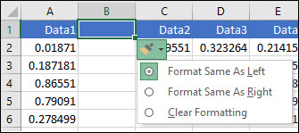
If the Insert Options button isn’t visible, then go to File > Options > Advanced > in the Cut, copy and paste group, check the Show Insert Options buttons option.

Insert rows

To insert a single row: Right-click the whole row above which you want to insert the new row, and then select Insert Rows.

To insert multiple rows: Select the same number of rows above which you want to add new ones. Right-click the selection, and then select Insert Rows.

Insert columns

To insert a single column: Right-click the whole column to the right of where you want to add the new column, and then select Insert Columns.

To insert multiple columns: Select the same number of columns to the right of where you want to add new ones. Right-click the selection, and then select Insert Columns.

Delete cells, rows, or columns

If you don’t need any of the existing cells, rows or columns, here’s how to delete them:

Select the cells, rows, or columns that you want to delete.
Right-click, and then select the appropriate delete option, for example, Delete Cells & Shift Up, Delete Cells & Shift Left, Delete Rows, or Delete Columns.

When you delete rows or columns, other rows or columns automatically shift up or to the left.

Tip: If you change your mind right after you deleted a cell, row, or column, just press Ctrl+Z to restore it.

Insert cells

To insert a single cell:

Right-click the cell above which you want to insert a new cell.
Select Insert, and then select Cells & Shift Down.

To insert multiple cells:

Select the same number of cells above which you want to add the new ones.
Right-click the selection, and then select Insert > Cells & Shift Down.

Need more help?

You can always ask an expert in the Excel Tech Community or get support in the Answers community.

How to Add a Column & Resize (Extend) a Table in Excel

This tutorial demonstrates how to extend a table by adding a column in Excel.

When working with tables in Excel, you can resize them by using Resize Table in the Table Design tab or by simply inserting a column.

Add Column in Table Design

Say you have the data table shown below with columns for SKU, Product, Month, and Sales Amount.

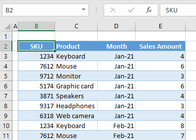
If you want to add Price and Total Sales to the table, you’ll need to add two columns to the right.

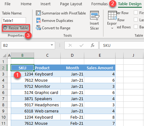
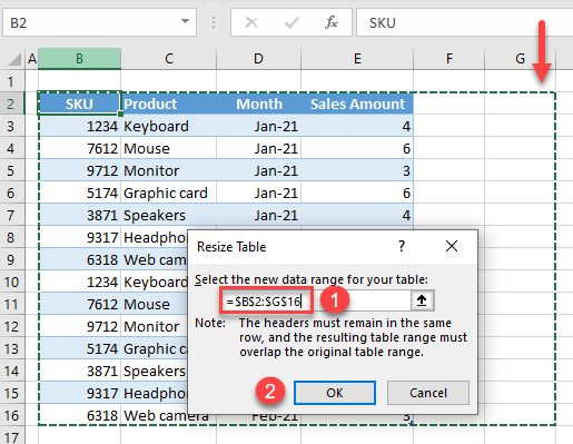
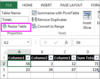
First, select the table by clicking on any cell in it. Then, in the Ribbon, go to the Table Design tab. In the Properties group, click Resize Table.

In the pop-up screen, change the range for the table and click OK.
Since you want to add two more columns to the right, expand the range for Columns F and G, and the new range is B2:G16. As you can see, when you enter a new range, the dashed line shows the table size.

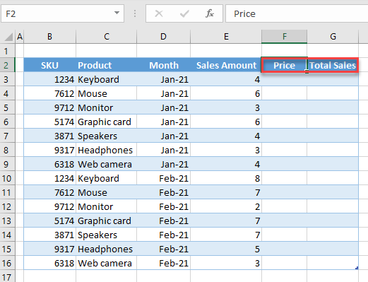
As a result, the table has two new columns (F and G) named Column1 and Column2.

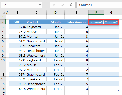
Finally, rename the columns. To rename Column1, enter Price in cell F2; and to rename Column2, enter Total Sales in G2.

Now you’ve resized the table and added the columns Price and Total Sales.

Insert Column

Another way to extend a table is to simply insert a new column.

Right-click the Sales Amount column, then go to Insert, and click on Table Column to the Right.

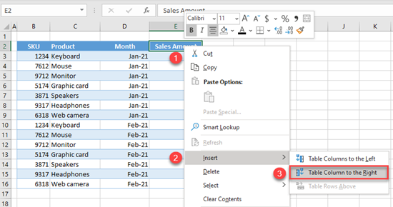
As a result, a new column (named Column1) is inserted to the right of the selected column (Sales Amount).

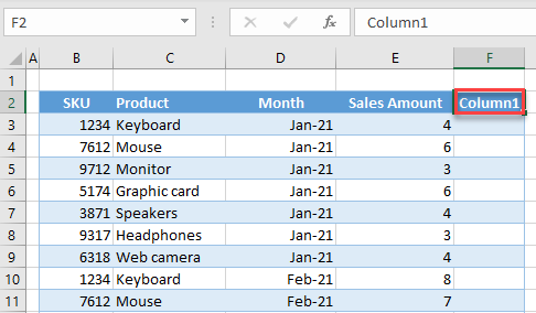
Then add one more column to the right in the same way.
If you rename these two columns Price and Total Sales, you arrive at the same result as with Resize Table.

Источник

Insert or delete rows, and columns

Insert and delete rows and columns to organize your worksheet better.

Note: Microsoft Excel has the following column and row limits: 16,384 columns wide by 1,048,576 rows tall.

Insert or delete a column

Select any cell within the column, then go to Home > Insert > Insert Sheet Columns or Delete Sheet Columns.

Alternatively, right-click the top of the column, and then select Insert or Delete.

Insert or delete a row

Select any cell within the row, then go to Home > Insert > Insert Sheet Rows or Delete Sheet Rows.

Alternatively, right-click the row number, and then select Insert or Delete.

Formatting options

When you select a row or column that has formatting applied, that formatting will be transferred to a new row or column that you insert. If you don’t want the formatting to be applied, you can select the Insert Options button after you insert, and choose from one of the options as follows:

If the Insert Options button isn’t visible, then go to File > Options > Advanced > in the Cut, copy and paste group, check the Show Insert Options buttons option.

Insert rows

To insert a single row: Right-click the whole row above which you want to insert the new row, and then select Insert Rows.

To insert multiple rows: Select the same number of rows above which you want to add new ones. Right-click the selection, and then select Insert Rows.

Insert columns

To insert a single column: Right-click the whole column to the right of where you want to add the new column, and then select Insert Columns.

To insert multiple columns: Select the same number of columns to the right of where you want to add new ones. Right-click the selection, and then select Insert Columns.

Delete cells, rows, or columns

If you don’t need any of the existing cells, rows or columns, here’s how to delete them:

Select the cells, rows, or columns that you want to delete.

Right-click, and then select the appropriate delete option, for example, Delete Cells & Shift Up, Delete Cells & Shift Left, Delete Rows, or Delete Columns.

When you delete rows or columns, other rows or columns automatically shift up or to the left.

Tip: If you change your mind right after you deleted a cell, row, or column, just press Ctrl+ Z to restore it.

Insert cells

To insert a single cell:

Right-click the cell above which you want to insert a new cell.

Select Insert, and then select Cells & Shift Down.

To insert multiple cells:

Select the same number of cells above which you want to add the new ones.

Right-click the selection, and then select Insert > Cells & Shift Down.

Need more help?

You can always ask an expert in the Excel Tech Community or get support in the Answers community.

Источник

Insert one or more rows, columns, or cells in Excel for Mac

You can insert rows above a selected row and columns to the left of a selected column. Similarly, you can insert blank cells above or to the left of the active cell on a worksheet. Cell references automatically adjust to match the location of the shifted cells.

Insert rows

Select the heading of the row above where you want to insert additional rows.

Tip: Select the same number of rows as you want to insert. For example, to insert five blank rows, select five rows. It’s okay if the rows contain data, because it will insert the rows above these rows.

Hold down CONTROL, click the selected rows, and then on the pop-up menu, click Insert.

Tip: To insert rows that contain data, see Copy and paste specific cell contents.

Insert columns

Select the heading of the column to the right of which you want to insert additional columns.

Tip: Select the same number of columns as you want to insert. For example, to insert five blank columns, select five columns. It’s okay if the columns contain data, because it will insert the columns to the left of these rows.

Hold down CONTROL, click the selected columns, and then on the pop-up menu, click Insert.

Tip: To insert columns that contain data, see Copy and paste specific cell contents.

Insert cells

When you insert blank cells, you can choose whether to shift other cells down or to the right to accommodate the new cells. Cell references automatically adjust to match the location of the shifted cells.

Select the cell, or the range of cells, to the right or above where you want to insert additional cells.

Tip: Select the same number of cells as you want to insert. For example, to insert five blank cells, select five cells.

Hold down CONTROL, click the selected cells, then on the pop-up menu, click Insert.

On the Insert menu, select whether to shift the selected cells down or to the right of the newly inserted cells.

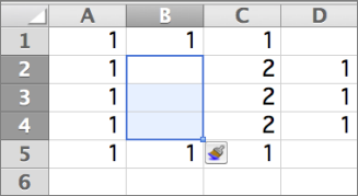
Here’s what happens when you shift cells left:

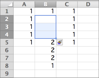
Here’s what happens when you shift cells down:

Tip: To insert cells that contain data, see Copy and paste specific cell contents.

Источник

Resize a table by adding or removing rows and columns

After you create an Excel table in your worksheet, you can easily add or remove table rows and columns.

You can use the Resize command in Excel to add rows and columns to a table:

Click anywhere in the table, and the Table Tools option appears.

Click Design > Resize Table.

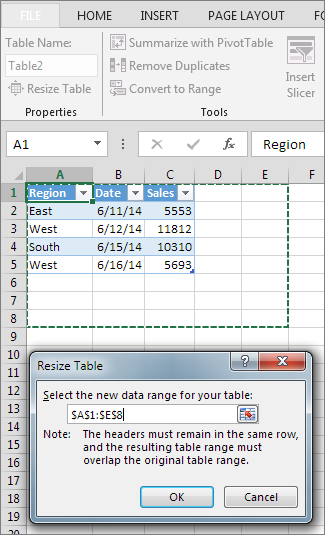
Select the entire range of cells you want your table to include, starting with the upper-leftmost cell.

In the example shown below, the original table covers the range A1:C5. After resizing to add two columns and three rows, the table will cover the range A1:E8.

Tip: You can also click Collapse Dialog to temporarily hide the Resize Table dialog box, select the range on the worksheet, and then click Expand dialog .

When you’ve selected the range you want for your table, press OK.

Add a row or column to a table by typing in a cell just below the last row or to the right of the last column, by pasting data into a cell, or by inserting rows or columns between existing rows or columns.

To add a row at the bottom of the table, start typing in a cell below the last table row. The table expands to include the new row. To add a column to the right of the table, start typing in a cell next to the last table column.

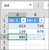
In the example shown below for a row, typing a value in cell A4 expands the table to include that cell in the table along with the adjacent cell in column B.

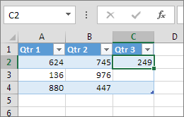
In the example shown below for a column, typing a value in cell C2 expands the table to include column C, naming the table column Qtr 3 because Excel sensed a naming pattern from Qtr 1 and Qtr 2.

To add a row by pasting, paste your data in the leftmost cell below the last table row. To add a column by pasting, paste your data to the right of the table’s rightmost column.

If the data you paste in a new row has as many or fewer columns than the table, the table expands to include all the cells in the range you pasted. If the data you paste has more columns than the table, the extra columns don’t become part of the table—you need to use the Resize command to expand the table to include them.

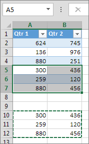
In the example shown below for rows, pasting the values from A10:B12 in the first row below the table (row 5) expands the table to include the pasted data.

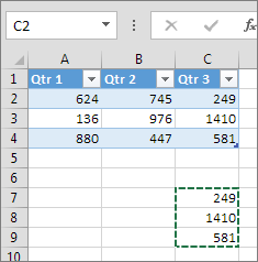
In the example shown below for columns, pasting the values from C7:C9 in the first column to right of the table (column C) expands the table to include the pasted data, adding a heading, Qtr 3.

Use Insert to add a row

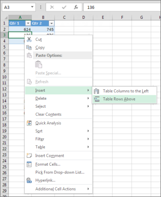
To insert a row, pick a cell or row that’s not the header row, and right-click. To insert a column, pick any cell in the table and right-click.

Point to Insert, and pick Table Rows Above to insert a new row, or Table Columns to the Left to insert a new column.

If you’re in the last row, you can pick Table Rows Above or Table Rows Below.

In the example shown below for rows, a row will be inserted above row 3.

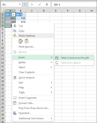
For columns, if you have a cell selected in the table’s rightmost column, you can choose between inserting Table Columns to the Left or Table Columns to the Right.

In the example shown below for columns, a column will be inserted to the left of column 1.

Select one or more table rows or table columns that you want to delete.

You can also just select one or more cells in the table rows or table columns that you want to delete.

On the Home tab, in the Cells group, click the arrow next to Delete, and then click Delete Table Rows or Delete Table Columns.

You can also right-click one or more rows or columns, point to Delete on the shortcut menu, and then click Table Columns or Table Rows. Or you can right-click one or more cells in a table row or table column, point to Delete, and then click Table Rows or Table Columns.

Just as you can remove duplicates from any selected data in Excel, you can easily remove duplicates from a table.

Click anywhere in the table.

This displays the Table Tools, adding the Design tab.

On the Design tab, in the Tools group, click Remove Duplicates.

In the Remove Duplicates dialog box, under Columns, select the columns that contain duplicates that you want to remove.

You can also click Unselect All and then select the columns that you want or click Select All to select all of the columns.

Note: Duplicates that you remove are deleted from the worksheet. If you inadvertently delete data that you meant to keep, you can use Ctrl+Z or click Undo on the Quick Access Toolbar to restore the deleted data. You may also want to use conditional formats to highlight duplicate values before you remove them. For more information, see Add, change, or clear conditional formats.

Make sure that the active cell is in a table column.

Click the arrow in the column header.

To filter for blanks, in the AutoFilter menu at the top of the list of values, clear (Select All), and then at the bottom of the list of values, select (Blanks).

Note: The (Blanks) check box is available only if the range of cells or table column contains at least one blank cell.

Select the blank rows in the table, and then press CTRL+- (hyphen).

You can use a similar procedure for filtering and removing blank worksheet rows. For more information about how to filter for blank rows in a worksheet, see Filter data in a range or table.

Select the table, then select Table Design > Resize Table.

Adjust the range of cells the table contains as needed, then select OK.

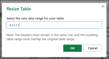
Important: Table headers can’t move to a different row, and the new range must overlap the original range.

Need more help?

You can always ask an expert in the Excel Tech Community or get support in the Answers community.

Источник

Download Article

Add values for an entire column or range

Download Article

Using AutoSum for One Column

Using SUM for One Column

Using SUM for Multiple Columns

Using SUMIF

Using the Status Bar

Using a Table

Tips

Warnings

This wikiHow will show you how to sum columns in Microsoft Excel for Windows or Mac. Use the AutoSum feature to quickly and easily find the total sum of a column’s values. You can also make your own formula using the SUM function! We’ll cover how to add the values of individual columns and entire cell ranges.

Things You Should Know

Go to Formulas > AutoSum to automatically add up a column.
Use the SUM function to add individual or multiple columns.
To add multiple columns, select the cell range containing each column you want to sum.

1
Click the cell directly below the values you want to sum. For example, if you have values in cells A1 through A5, you would click A6.^[1]
- If you’re just getting started with Excel, check out our intro guides for making a spreadsheet and formatting a spreadsheet.
2

Click the Formulas tab. This will display various formula options in the top bar.

Advertisement
3

Click AutoSum. This will open a drop down menu with AutoSum options.
4

Click Sum. This will automatically create a SUM function that adds the values of the column. You’ll see the values that are going to be summed in a highlighted selection box.
5

Press ↵ Enter or ⏎ Return on your keyboard. This will confirm the SUM formula and show you the sum total in the cell you selected.

1
Click a cell below the column you want to add up. Doing so will place your cursor in the cell. This method uses the SUM function, which adds all of the values in a given cell range.
- If you’re looking for subtraction information, check out our guide to subtracting in Excel.
2

Enter the «SUM» function. Type =SUM() into the cell.
3
Enter the column’s range. Type the top cell in the column, a colon, and the bottom cell in the column into the parentheses.
- For example, if you’re adding values in the A column and you have data in cells A2 through A10, you would type in the following: =SUM(A2:A10)
- If your dataset has a header row, don’t include the header in the SUM formula.
4

Press ↵ Enter or ⏎ Return. This will display the sum of the column in your selected cell.
5
Create the sums of the other columns you want to add. You can create SUM formulas for each column, or copy the first formula:
- To quickly sum other columns of the same length, you can press Ctrl+c (Windows) to copy the cell with the SUM formula, then press Ctrl+v (Windows) to paste it under the other columns.
  - On Mac, these shortcuts are ⌘ Cmd+c and ⌘ Cmd+v respectively.
  - Pasting the formula will automatically change the cell references to the column that corresponds with where you pasted the formula.

1
Determine which of your columns is the longest. This method adds up multiple columns in one formula. In order to include all of the cells in the longest column, you’ll need to know to which row the column extends.
- For example, if you have three columns and the longest one has values from row 1 through row 20, your formula will need to include rows 1 through 20 for each column you want to add even if this includes blank cells.
2

Determine your beginning and ending columns. If you’re adding the A column and the B column, for example, your beginning column is the A column and your ending column is the B column.
3

Select a blank cell. Click the cell in which you want to display the sum of your columns.
4

Enter the «SUM» command. Type =SUM() into the cell.
5
Enter the cell range. For a range of cells, the left cell in the range is the top-left cell, and the right cell is the bottom-right cell. These two cells define the range.
- In other words, type the first column letter, the first row number, a colon, the last column letter, and the last row number.
- For example, if you’re adding columns A, B, and C, and your longest column stretches to row 20, you would enter the following: =SUM(A1:C20)
6

Press ↵ Enter or ⏎ Return. Doing so will display the sum of all of the columns in your selected cell.

1

Click a cell below the column you want to add up. Doing so will place your cursor in the cell. This method uses the SUMIF function, which allows you to add values in a data range if they meet a certain criteria.^[2]
2
Enter the «SUMIF» function. Type =SUMIF() into the cell.
- SUMIF has three arguments: range, criteria, [sum_range]. The [sum_range] argument is optional and used to specify a different range to sum values in. The criteria argument will check the range specified in the first argument.
3
Enter the column’s range and a comma. Type the top cell in the column, a colon, and the bottom cell in the column into the parentheses.
- For example, if you’re checking the values in the A column and you have data in cells A2 through A10, you would type in the following: =SUMIF(A2:A10,)
- If your dataset has a header row, don’t include the header in the SUM formula.
4
Enter the criteria you want to check. Place the criteria as the second argument after the comma. This can be a cell reference, text, number, expression, or function. Each cell in the specified range will be checked using this criteria. If the criteria is met, it will be added to the total sum. Here are a few examples:
- =SUMIF(A2:A10, 7) would check whether a value equals 7.
- =SUMIF(A2:A10, "<10") would check whether a value is less than 10. Note that logical criteria needs quotation marks.
- =SUMIF(A2:A10, "cat") would check whether the value is the word «cat».
5
Enter a comma and a sum range (optional). Place a comma after the criteria argument, then type a sum range. The sum range needs to be the same shape and size as the range in the first argument. SUMIF will check the criteria in the range and add the corresponding value in the sum range.
- For example, if you had 9 purchases in A2:A10 and their corresponding prices in B2:B10, you could sum the prices of purchase called «food» using this formula:
- =SUMIF(A2:A10, "food", B2:B10)
6

Press ↵ Enter or ⏎ Return. This will display the sum in your selected cell.

1

Click a column letter to see the sum of its values. This is the letter header located above the spreadsheet cells. The entire column will be highlighted.
2

Look at the status bar to see the sum. At the bottom of Excel is the status bar. The sum total of the values in the column will be displayed next to «sum:».

1

Select your dataset. Click and drag from the top left to the bottom right of your dataset to select it. This method changes the dataset into a table, to which you can add a total row.^[3]
2

Click the Home tab. It’s at the top of the Excel window.
3

Click Format as Table. A drop down menu will appear with table options.
4

Select a table style. You can select from a variety of colors and formats. A small window titled «Create table» will appear after selecting a style.
5

Check the box next to «My table has headers» (if needed). If your dataset has a header row, select this option to format the table correctly. Otherwise, uncheck the box.
6

Click OK. This will change the dataset into a table.
7

Click the Table Design tab. It’s at the top of the Excel window.
8

Check the box next to «Total Row». This is an option in the «Table Style Options» section of the Table Design tab.^[4]
9

Click the cell in the total row in the column you want to sum. A drop down arrow will appear next to the cell. For example, if your data is in A2:A10 and the total row is in row 11, you would click A11.
10

Click the drop down arrow ▼. This will display a down down menu with total options.
11

Select Sum. This is an option in the total drop down menu. A sum total for that column will appear in the cell. You’re done!

Add New Question

Question

How do I copy a formula?

Right click on the cell with the formula, select «Copy,» and then paste the formula into the desired cell. Keep in mind you may have to manipulate the formula in the new cell if the columns are not the same length.
Question

How do I multiply two cells?

To multiply two cells use the * key to multiply by pressing shift 8, and type it in the cell you want, e.g. A1*B5.

Ask a Question

200 characters left

Include your email address to get a message when this question is answered.

Submit

To total up a single column, you can enter the column’s first value, a colon, and the last value into the SUM command. For example, to add cells A1, A2, A3, A4, and A5 together, you would type =SUM(A1:A5) into an empty cell.
For an advanced Excel function, check out our guide on using VLOOKUP.

Thanks for submitting a tip for review!

Changing a column cell’s contents will cause the cell in which you’re displaying the columns’ total to change its value as well.

About This Article

Thanks to all authors for creating a page that has been read 157,984 times.

Is this article up to date?

Источник

Adding a column in Excel means inserting a new column to the existing dataset. Besides inserting, one may need to delete, hide, unhide, and move rows or columns. Such modifications help in structuring and organizing the dataset. As a result, it is essential to be aware of the techniques related to these alterations.

For example, while preparing a consolidated balance sheet, Mr. X realizes that the data related to the previous year is missing. To include this data, he wants to insert a new column. Here, the method of inserting a column comes into use.

Excel provides different ways of performing actions on a dataset. This article discusses the most appropriate and effective methods of working with data. It covers the following aspects: –

Insert Excel columns (alternate methods and shortcuts)
Delete columns and rows
Hide and unhide rows or columns
Move rows or columns

Apart from inserting columns in Excel, the remaining topics have been covered in brief.

How to Add/Insert Columns in Excel?
- Example #1–Add Columns in Excel
- Example #2–Alternate Method to Insert Rows and Columns in Excel
- Example #3–Hide and Unhide Columns & Rows in Excel
- Example #4–Move Rows or Columns in Excel
Shortcuts to Insert Columns in Excel
Frequently Asked Questions
Recommended Articles

How to Add/Insert Columns in Excel?

Below are some examples through which you may learn how to add and insert columns in Excel.

Example #1–Add Columns in Excel

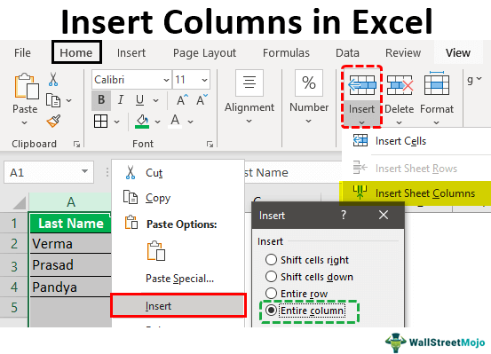
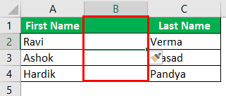
The following table shows the first and the last names in columns A and B, respectively. We want to insert a new column (column B) between these names, which will display the middle name.

The steps to insert a new column (column B) between two existing columns (columns A and B) are listed as follows:

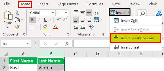
Step 1: Select any cell of column B. Alternatively, one can also select column B, as shown in the following image. Further, click the “Insert” drop-down from the “Home” tab of the Excel ribbonThe ribbon is an element of the UI (User Interface) which is seen as a strip that consists of buttons or tabs; it is available at the top of the excel sheet. This option was first introduced in the Microsoft Excel 2007.read more. Finally, select “Insert Sheet Columns.”

Note: To select a column, click its label or header on top.

Step 2: A new column (column B) is inserted between the columns containing the first and the last names. As a result, the data (last name) of the previous column B (shown in step 1) now shifts to column C.

Note: Excel inserts a column immediately preceding the column of the selected cell. Hence, one must always choose a cell accordingly. If a column is selected, Excel inserts a column preceding it.

Example #2–Alternate Method to Insert Rows and Columns in Excel

Working on the data of example #1, we need to insert a middle name column using the following methods:

a) Select and right-click a cell

b) Select and right-click a column

a) The steps for inserting a column after selecting and right-clicking a cell are listed as follows:

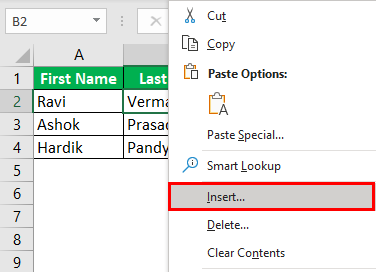
Step 1: Select any cell of column B. This is because a column preceding column B is to be inserted. Right-click the selection and choose “insert,” as shown in the following image.

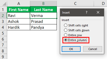
Step 2: The “Insert” dialog box appears. Select “Entire column” to insert a new column.

Note: For inserting a new row, select “Entire row.”

Step 3: A new column (column B) for typing middle names has been inserted.

b) The steps for inserting a column after selecting and right-clicking a column are listed as follows:

Step 1: Select the entire column B. That is because a column preceding column B is to be inserted. Right-click the selection and choose “Insert,” as shown in the following image.

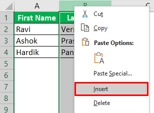
Step 2: A new column B is inserted. The same has been shown under step 3 of method a.

Note: Select the entire row preceding which a new row is inserted for inserting rows. Right-click the selection and choose “Insert.” The same is shown in the following image.

Example #3–Hide and Unhide Columns & Rows in Excel

Working on the data of example #1, we want to perform the following tasks:

a) Hide columns A and B or rows 3 and 4 by right-clicking

b) Hide column A by using the “format” drop-down

c) Unhide columns B and C by right-clicking

a) The steps to hide the columns A and B or rows 3 and 4 by right-clicking are listed as follows:

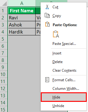
Step 1: Select columns A and B. Right-click the selection and choose “hide,” as shown in the next image.

Note 1: To select a row or column, click the row number (to the left) or the column label (on top).

Note 2: Multiple adjacent rows or columns can be selected by dragging across the row and column headings. Alternatively, hold the “Shift” key while selecting the rows or columns.

Note 3: We can select non-adjacent rows or columns by holding the “Ctrl” key while making the selections.

Step 2: Columns A and B will be hidden. Likewise, select rows 3 and 4. Right-click the selection and choose the “Hide” option from the context menu. The same is shown in the following image.

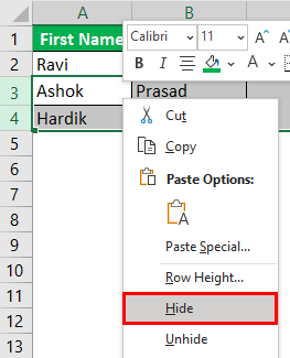
It will hide rows 3 and 4.

b) The steps to hide column A by using the “format” drop-down are listed as follows:

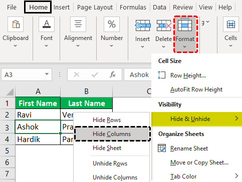
Step 1: Select any cell of column A. Click the “Format” drop-down under the “Home” tab of the Excel ribbon. Next, select “Hide Columns” under the “Hide & Unhide” option.

The same is shown in the following image.

Note: Alternatively, select the relevant column to be hidden. Click “Hide columns” under the “Hide & Unhide” option.

Step 2: We will hide the column of the selected cell, column A. Likewise, to hide rows, select the relevant row. Then, choose “Hide Rows” from the “Hide & Unhide” option of the “Format” drop-down.

c) The steps to unhide columns B and C by right-clicking are listed as follows:

Step 1: Select the unhidden columns (A and D) immediately before and after the hidden columns (B and C). Right-click the selection and choose “Unhide.”

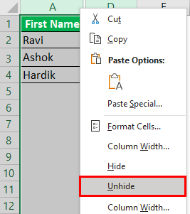
Step 2: The columns B and C will be unhidden. The dataset appears as shown in step 1 of task b.

Likewise, unhide rows by selecting the “Unhide rows” (immediately before and after the hidden rows) and clicking “Unhide” from the context menu.

Example #4–Move Rows or Columns in Excel

Working on the data of example #1, we want to move column B (last name) to precede column A (first name).

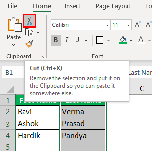
The steps to move column B are listed as follows:

Step 1: Select column B, which is to be moved. Cut it in either of the following ways:

Press “Ctrl+X.”
Click the scissors icon from the “Clipboard” group of the “Home” tab.

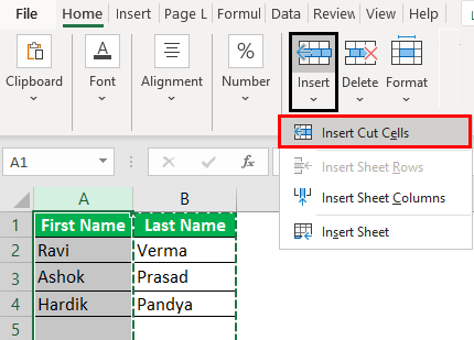
Step 2: Select column A, where the data of column B is to be pasted. Right-click the selection and choose “Insert Cut Cells.”

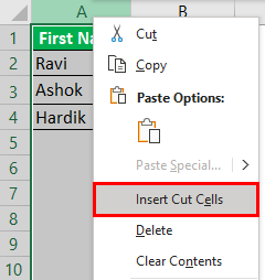
Alternatively, select “Insert Cut Cells” from the “Insert” drop-down of the “Home” tab. The same is shown in the following image.

Note: The “Insert Cut Cells” option will be visible once the selected cells have been cut.

Step 3: The data of column B is pasted into column A. Hence, the first column (column A) now contains the last names. The data of the initial column A (first name) automatically shifts to column B.

The same is shown in the following image.

Note: A row can be selected, cut, and pasted to the desired location. Select the “Insert Cut Cells” option from the “Insert” drop-down of the “Home” tab for pasting.

Shortcuts to Insert Columns in Excel

Let us go through the two shortcuts for inserting columns and rows.

a) Shortcut for inserting with the “Insert” drop-down of the “Home” tab

The excel shortcutAn Excel shortcut is a technique of performing a manual task in a quicker way.read more for inserting a row or column with the “Insert” drop-down works as follows:

Select a cell preceding which a row or column is inserted.
Click the “Insert” drop-down from the “Cells” group of the “Home” tab.
Press “R” to insert a row or “C” to insert a column

A new row or column is inserted depending on the third pointer’s key.

Note: Under the “Insert” drop-down, the “R” of “insert sheet rows” and the “C” of “insert sheet columns” are underlined. Hence, these keys work as shortcuts for inserting rows and columns.

b) Shortcut for inserting with right-click

The shortcut for inserting a row or column with right-click works as follows:
Select a cell preceding which a row or column is inserted.
Right-click the selection and press “I.” The “Insert” dialog box opens.
Press “R” to insert a row or “C” to insert a column.
Press the “Enter” key.

A new row or column is inserted depending on the third pointer’s key.

Note: If the “Insert” dialog box does not open in step 2, press the “Enter” key after pressing “I.” It opens the “Insert” dialog box.

Frequently Asked Questions

1. What does it mean to insert a column? How is it done in Excel?

Inserting a column refers to adding a new column to an existing dataset. This new column may contain additional data that can be important for the end-user.

Additionally, there is a possibility that a column has been omitted by mistake. In such cases, inserting a column will be helpful.

The steps to insert a column in Excel are listed as follows:

a. Select the column preceding which a new column is to be inserted.
b. Right-click the selection and choose “Insert” from the context menu.

It will insert the new column immediately before the selected column.

Note: To select a column, click its header (label) on top.

2. How to insert a column in Excel by using a shortcut?

Let us insert a new column E in Excel. The steps to insert a column (column E) by using a shortcut are listed as follows:

a. Select the existing column E.
b. Press the keys “Ctrl+Shift+plus sign(+)” together to insert a column.

It will insert the new column E. The data of the initial column E now shifts to column F.

Note 1: One must select a column carefully. That is because Excel inserts a column preceding the selected column.

Note 2: As an alternative to step a, one can select any cell of column E. After that, press “Ctrl+space” to select the entire column E.

3. How to insert multiple adjacent columns in Excel?

Let us insert columns D, E, and F in Excel. The steps to insert multiple columns (D, E, and F) are listed as follows:

a. Select as many columns in the existing dataset as the number of the new columns to be inserted. So, select the current columns D, E, and F.
b. Press the keys “Ctrl+Shift+plus sign(+)” together.

It will insert the blank columns D, E, and F. The initial columns D, E, and F data shift to columns G, H, and I.

Note 1: Alternative to step a: select adjacent cells of columns D, E, and F. These cells should be in one row. Further, press “Ctrl+space.” As a result, columns D, E, and F will be selected.

Note 2: To select multiple adjacent columns (in step a), drag across the column headings. Alternatively, hold the “Shift” key while selecting the columns.

Note 3: Alternative to step b: right-click the selection and choose “Insert.”

Insert New Columns in Excel

In this tutorial, I will cover the following methods/scenarios to insert new columns in Excel:

Insert one new column (using keyboard shortcut or options in the ribbon)
Add multiple new columns
Add non-adjacent columns at one go
Insert new columns after every other column
Insert a New Column in an Excel Table

Insert a New Column (Keyboard Shortcut)

Suppose you have a dataset as shown below and you want to add a new column to the left of column B.

Below is the keyboard shortcut to insert a column in Excel:

Control Shift + (hold the Control and Shift keys and press the plus key)

Command + I if you’re using Mac

Below are the steps to use this keyboard shortcut to add a column to the left of the selected column:

Select a cell in the column to the left of which you want to add a new column
Use the keyboard shortcut Control Shift +
In the Insert dialog box that opens, click the Entire Column option (or hit the C key)
Click OK (or hit the Enter key).

The above steps would instantly add a new column to the left of the selected column.

Another way to add a new column is to first select an entire column and then use the above steps. When you select an entire column, using the Control Shift + shortcut will not show the insert dialog box.

It will just add the new column right away.

Below is the keyboard shortcut to select the entire column (once you select a cell in the column):

Control + Spacebar (hold the Control key and press the space bar key)

Once you have the column selected, you can use Control Shift + to add a new column.

If you’re not a fan of keyboard shortcuts, you can also use the right-click method to insert a new column. Simply right-click on any cell in a column, right-click and then click on Insert. This will open the Insert dialog box where you can select ‘Entire Column’.

This would insert a column to the left of the column where you selected the cell.

Add Multiple New Columns (Adjacent)

In case you need to insert multiple adjacent columns, you can either insert one column and time and just repeat the same process (you can use the F4 key to repeat the last action), or you can insert all these columns at one go.

Suppose you have a dataset as shown below and you want to add two columns to the left of column B.

Below are the steps to do this:

Select two columns (starting with the one on the left of which you want to insert the columns)
Right-click anywhere in the selection
Click on Insert

The above steps would instantly insert two columns to the left of Column B.

In case you want to insert any other number of columns (say 3 or 4 or 5 columns), you select that many to begin with.

Add Multiple New Columns (Non-Adjacent)

The above example is quick and fast when you want to add new adjacent columns (i.e., a block of 3 adjacent columns as shown above).

But what if you want to insert columns but these are non-adjacent.

For example, suppose you have a dataset as shown below, and you want to insert one column before Column B and one before Column D.

While you can choose to do this one by one, there is a better way.

Below are the steps to add multiple non-adjacent columns in Excel:

Select the columns where you want to insert a new column.
Right-click anywhere in the selection
Click on Insert.

The above steps would instantly insert a column to the left of the selected columns.

Insert New Columns After Every Other Column (Using VBA)

Sometimes, you may want to add a new column after every other column in your existing dataset.

While you can do this manually, if you’re working with a large dataset, this can take some time.

The faster way of doing this would be to use a simple VBA code to simply insert a column after every column in your dataset.

Sub InsertColumn()
'Code created by Sumit Bansal from trumpexcel.com

Dim ColCount As Integer
Dim i As Integer

StartCol = Selection.Columns.Count + Selection.Columns(1).Column
EndCol = Selection.Columns(1).Column

For i = StartCol To EndCol Step -1
    Cells(1, i).EntireColumn.Insert
Next i

End Sub

The above code will go through each column in the selection and insert a column to the right of the selected columns.

You can add this code to a regular module and then run this macro from there.

Or, if you have to use this functionality regularly, you can also consider adding it to Personal Macro Workbook and then adding it to the Quick Access Toolbar. This way, you will always have access to this code and can run it with a single click.

Note: The above code also works when you have the data formatted as an Excel table.

Add a Column in an Excel Table

When you convert a dataset into an Excel Table, you lose some of the flexibility that you have with regular data when it comes to inserting columns.

For example, you can not select non-contiguous columns and insert columns next to it at one go. You will have to do this one by one.

Suppose you have an Excel Table as shown below.

To insert a column to the left of column B, select any cell in the column, right-click, go to the Insert option and click on ‘Table Columns to the left’.

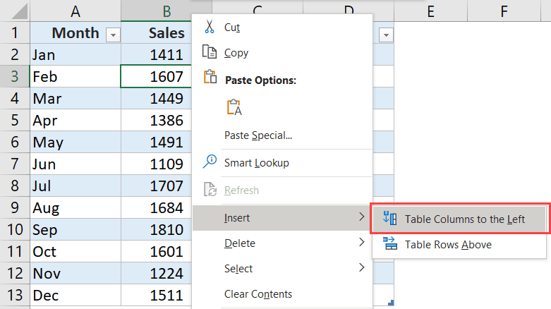
This will insert a column to the left of the selected cell.

In case you select a cell in Column B and one in Column D, you will notice that the ‘Table Columns to the left’ option is grayed out. In this case, you will have to insert columns one by one only.

What’s surprising is that this works when you select non-contiguous rows, but not with columns.

So these are some of the methods you can use to insert new columns in Excel. All the methods covered in this tutorial will also work if you want to insert new rows (the VBA code would need some modification though).

Hope you found this tutorial useful!

You may also like the following Excel tutorials:

How to Sum a Column in Excel
How to Unhide COLUMNS in Excel
How to Move Rows and Columns in Excel
How to Compare Two Columns in Excel (for matches & differences)
How to Freeze Multiple Columns in Excel?

Источник

Insert or delete a column

Insert or delete a row

Formatting options

Insert rows

Insert columns

Delete cells, rows, or columns

Insert cells

Need more help?

See Also

Need more help?

How to Add a Column & Resize (Extend) a Table in Excel

Add Column in Table Design

Insert Column

Insert or delete rows, and columns

Insert or delete a column

Insert or delete a row

Formatting options

Insert rows

Insert columns

Delete cells, rows, or columns

Insert cells

Need more help?

Insert one or more rows, columns, or cells in Excel for Mac

Insert rows

Insert columns

Insert cells

Resize a table by adding or removing rows and columns

Need more help?

Things You Should Know

About This Article

Is this article up to date?

Table of contents

How to Add/Insert Columns in Excel?

Example #1–Add Columns in Excel

Example #2–Alternate Method to Insert Rows and Columns in Excel

Example #3–Hide and Unhide Columns & Rows in Excel

Example #4–Move Rows or Columns in Excel

Shortcuts to Insert Columns in Excel

Frequently Asked Questions

Recommended Articles

Insert New Columns in Excel

Insert a New Column (Keyboard Shortcut)

Add Multiple New Columns (Adjacent)

Add Multiple New Columns (Non-Adjacent)

Insert New Columns After Every Other Column (Using VBA)

Add a Column in an Excel Table