
Используйте Excel Power Query (Получить & Transform( Power Query) для подключения к серверу базы данных SQL Server Analysis Services (OLAP ).
-
На вкладке Данные нажмите кнопку Получить данные > из базы > из базы SQL Server служб Analysis Services (Импорт). Если вы не видите кнопку Получить данные, нажмите кнопку Новый запрос > из базы данных > из базы данных analysis Services SQL Server.
-
Ввести имя сервера и нажмите кнопку ОК.
Примечание: Вы можете ввести имя конкретной базы данных, а также добавить запрос многоязовой или DAX.
-
В области Навигатор выберите базу данных, а затем куб или таблицы, которые вы хотите соединить.
-
Нажмите кнопку Загрузить, чтобы загрузить выбранную таблицу, или изменить, чтобы выполнить дополнительные фильтры и преобразования данных перед загрузкой.
В Excel 2010 и 2013 года существует два способа создания подключения к базе данных SQL Server analysis Services (OLAP). Рекомендуемый способ — использовать Power Query, который доступен при скачии надстройки Power Query. Если вы не можете скачать Power Query, воспользуйтесь мастером подключения к данным.
Power Query
-
На ленте Power Query щелкните Из базы > Из SQL Server служб Analysis Services.
-
Ввести имя сервера и нажмите кнопку ОК.
Примечание: Вы можете ввести имя конкретной базы данных, а также добавить запрос многоязовой или DAX.
-
В области Навигатор выберите базу данных, а затем куб или таблицы, которые вы хотите соединить.
-
Нажмите кнопку Загрузить, чтобы загрузить выбранную таблицу, или изменить, чтобы выполнить дополнительные фильтры и преобразования данных перед загрузкой.
Мастер подключения к данным
-
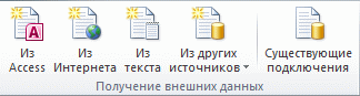
На вкладке Данные в группе Внешние данные нажмите кнопку Из других источников ивыберите из служб Analysis Services.

-
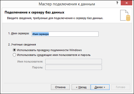
В мастере подключения к даннымвведите имя сервера и выберите параметр входа. Нажмите кнопку Далее.
-
Выберите базу данных и таблицу или куб, к которой нужно подключиться, и нажмите кнопку Далее.
-
Введите имя и описание нового подключения и нажмите кнопку Готово, чтобы сохранить его.
-
В диалоговом оке Импорт данных выберите способ и место извлечения данных. Начиная с Excel 2013 г., вы также можете сохранить данные в модели данных.
Use Excel’s Get & Transform (Power Query) experience to connect to a SQL Server Analysis Services (OLAP) database server.
-
Click the Data tab, then Get Data > From Database > From SQL Server Analysis Services Database (Import). If you don’t see the Get Data button, then click New Query > From Database > From SQL Server Analysis Services Database.
-
Input the Server name and press OK.
Note: You have the option of entering a specific database name, and you can add an MDX or DAX query.
-
In the Navigator pane select the database, then the cube or tables you want to connect.
-
Click Load to load the selected table, or click Edit to perform additional data filters and transformations before loading it.
In Excel 2010 and 2013, there are two methods of creating a connection to a SQL Server Analysis Services (OLAP) database. The recommended method is to use Power Query, which is available if you download the Power Query add-in. If you can’t download Power Query, you can use the Data Connection Wizard.
Power Query
-
In the Power Query ribbon, click From Database > From SQL Server Analysis Services Database.
-
Input the Server name and press OK.
Note: You have the option of entering a specific database name, and you can add an MDX or DAX query.
-
In the Navigator pane select the database, then the cube or tables you want to connect.
-
Click Load to load the selected table, or click Edit to perform additional data filters and transformations before loading it.
Data Connection Wizard
-
On the Data tab, in the Get External Data group, click From Other Sources, and then click From Analysis Services.
-
In the Data Connection Wizard, enter the Server name, and select a login option. Click Next.
-
Select the database and table or cube that you want to connect to, then click Next.
-
Enter a name and description for the new connection, and press Finish to save it.
-
In the Import Data dialog, select an option for how you want the data to be retrieved, and where you want to place the it. Beginning with Excel 2013, you also have the option to save the data to the Data Model.
Introduction
In SSAS, when I offer Power BI, Reporting Services, PowerPivot or SharePoint to connect to SSAS, the business analysts look scared. On the other hand, if I talk about MS Excel, everybody seems so happy and comfortable with it.
Excel is still the most popular spreadsheet in the world even when there are a lot of free spreadsheets like OpenOffice and LibreOffice to download, in the BI world, Excel is still the most popular.
Since then the usage is still growing. Office 365, a new version of Office in the cloud is growing each day and you can connect from your Android or iPhone device and store the information in OneDrive, the Microsoft storage.
In this article, we are going to learn how to connect to SSAS using Excel and create some reports on it.
Requirements
- SSAS multidimensional database installed
- SQL Server 2016 Installed
- SSDT
- The AdventureworksDW database
- SSMS 2017 installed
- Excel Installed
- An SSAS database already installed. You can use our sample created in our article How to build a cube from scratch using SQL Server Analysis Services (SSAS)
Getting started
In your machine, open Excel:
In the menu, go to data. Select the icon From other sources and select from Analysis Services. This option will create a PivotTable with the SSAS cube information:
Write the name of the SSAS Server. Your current Windows credentials should have access to SSAS server. You can also use a specified username and password:
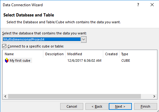
In SSAS, you have the database (MultidimensionalProject4) and inside the database, you have cubes (My first cube). Select your database and cube and press next:
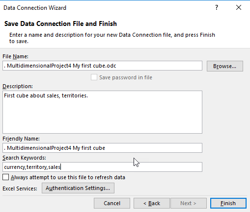
The information is stored in an ODC file (Office Data Connector) this file is an xml file used to connect to different data sources. In this case to SSAS. You can specify a description, keywords and the file name here. The description and keywords may be useful to identify the connection and to search it:
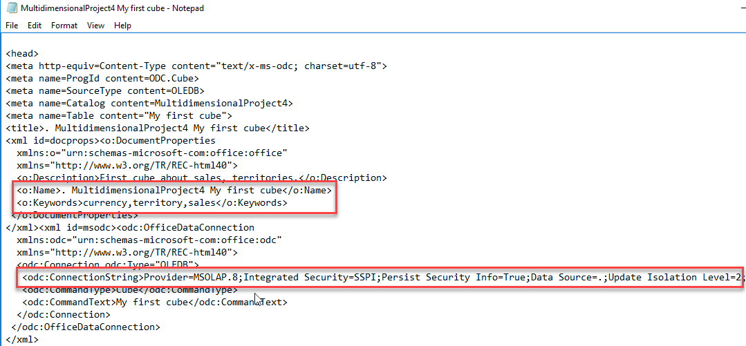
The ODC file contains the name of the database, keywords, connection information and type of connection (OLEDB):
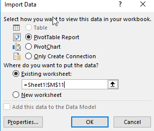
You can create a report, a chart or just create a connection. Select the option, PivotTable Report. You can also select the sheet where the report will be displayed or create a new one:
A PivotTable will be created in Excel:
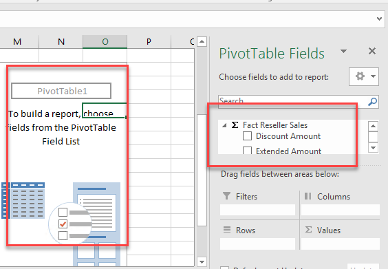
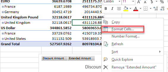
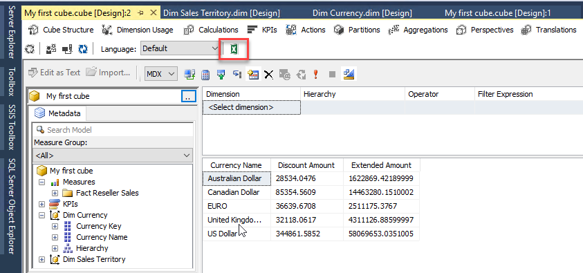
In your fact table (fact reseller sales in my example) check your measures to be displayed (Discount Amount and the extended amount in my example):
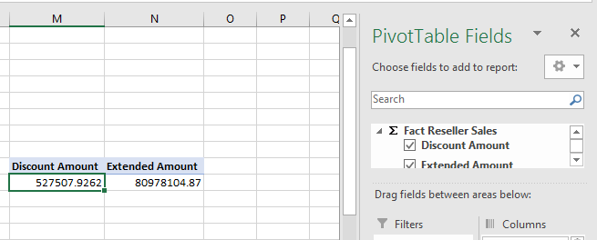
You will be able to visualize the total discount and extended amount. Double click the discount amount:
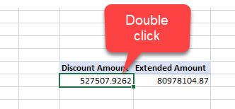
A new sheet will be created with detailed Discount amount information. It will display the first 1000 rows:
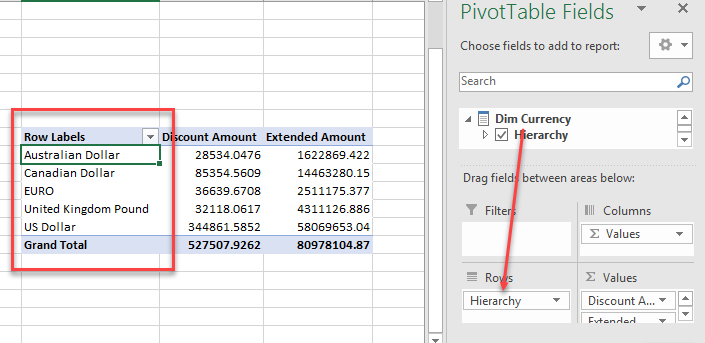
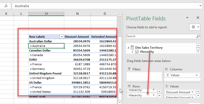
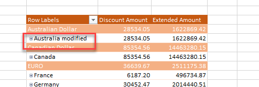
Drag and drop the Dim currency to the rows section. This will display discount and extended amounts grouped by currency:
We will drag and drop the Dim Sales Territory to the Rows to group the Discount Amount and Extended Amount by territory and currency:
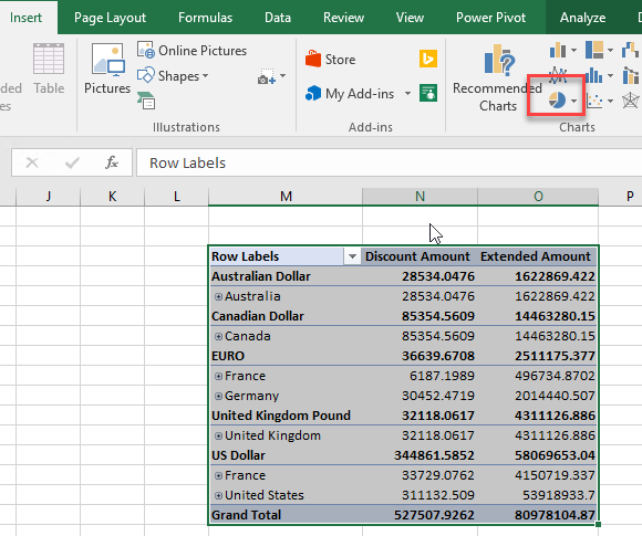
We will now create a graph based on the current information. Select the report information and go to Insert and select the pie icon:
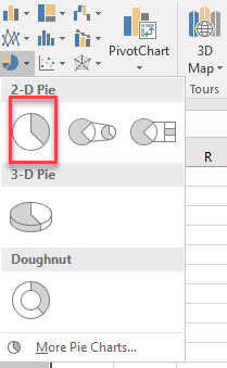
Select the graph that you want to use:
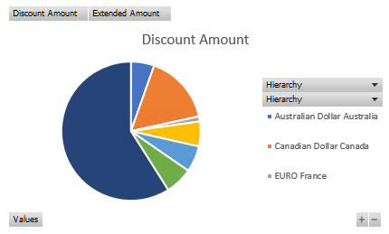
You will now have a graph about the discount amount by currency type:
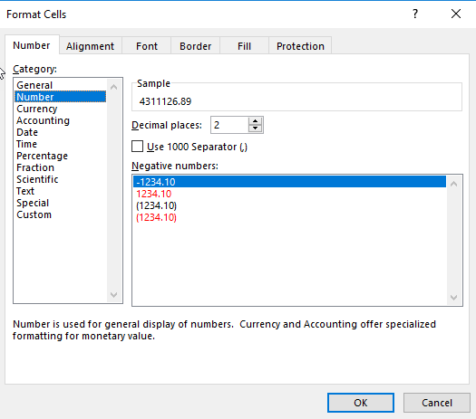
You can modify the format of your cells. If you right click the format cells, you can modify the format:
For example, we can change the numbers display in number format with 2 decimals:
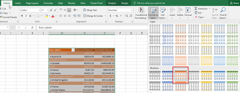
You can easily change the table format using Excel:
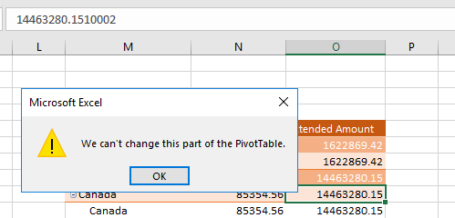
If you want to edit the numbers, you will receive a warning and you will not be able to change the data:
You can modify the labels like the country names:
If you right click on the numbers, you will find the option to configure PivotTable options:
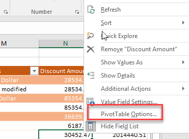
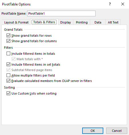
In show and filters tab, you can configure if you want to see the totals for row and columns, use a custom list and more.
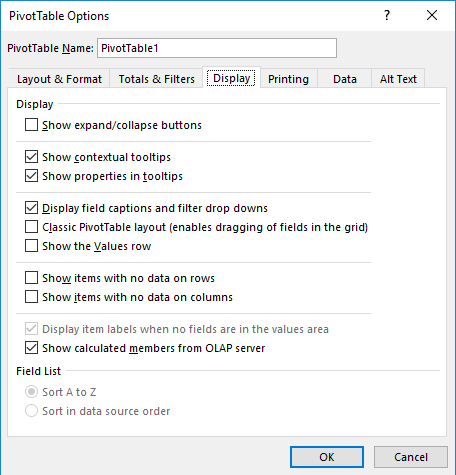
In display tab, you can configure if you want to see expand and collapse buttons, show calculated members and more:
If you have SSDT, there is an option to connect to Excel and create the ODC directly. This option is useful if you have SSDT and Excel on the same machine. If you only have Excel, the previous steps should be used.
In SSDT, go to the Cube and go to Browser tab:
There is an Excel icon to Analyze in Excel the data. Click it:
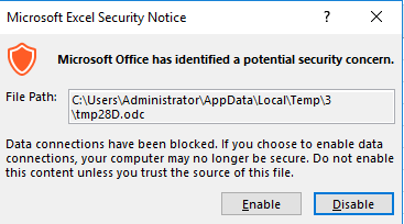
You may receive a warning in Excel about a potential security problem. It is the ODC file being created automatically. You can trust it. Press Enable:
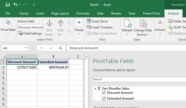
The Excel will be connected automatically and you can work as we did before:
Conclusion
In this article, we learned how to create reports in Excel based on the cube information in SSAS. We first need to create a Data the connection and then we drag and drop the measures and dimensions.
Excel is pretty simple and intuitive to create reports. You cannot modify the data, but you can modify the label names at the customer side.
The connection is made using an ODC file which can be modified manually or using Excel itself. It is necessary to have a Windows credentials to SSAS in the account that is using Excel.
There are other alternatives to have reports in Excel like using Reporting Services or Power BI to create reports and then export to Excel. However, this option. in my opinion is the best if the user has experience in Excel and does not have experience in other BI technologies. The learning curve is really short.
We also learned that there is an option in SSDT to create the connection immediately. With that option, you do not need to write credential information to connect to SSAS from Excel.
References
For more information about connecting to SSAS using Excel refer to these links:
- Get data from Analysis Services
- Analyze in Excel
- Connect to SQL Server Analysis Services Database (Import)
- Querying SSAS cubes in Excel
- Author
- Recent Posts

Daniel Calbimonte is a Microsoft Most Valuable Professional, Microsoft Certified Trainer and Microsoft Certified IT Professional for SQL Server. He is an accomplished SSIS author, teacher at IT Academies and has over 13 years of experience working with different databases.
He has worked for the government, oil companies, web sites, magazines and universities around the world. Daniel also regularly speaks at SQL Servers conferences and blogs. He writes SQL Server training materials for certification exams.
He also helps with translating SQLShack articles to Spanish
View all posts by Daniel Calbimonte
Although it is well-known how to create a tabular database in PowerPivot, it is less obvious that there are several useful options for retrieving SSAS tabular data into Excel. This provides an easy way of manipulating, visualizing and analyzing the data without needing to know the details of SSAS and the tabular model.
Until recently, most of the talk about tabular data revolved around PowerPivot, an Excel add-in that brings powerful in-memory data crunching to the spreadsheet environment. Creating a tabular database in PowerPivot, and by extension, within Excel, is a fairly prescribed process that involves retrieving data from one or more data sources-most notably SQL Server databases-and creating one or more tables based on that data.
Despite all the attention paid to PowerPivot and its tabular databases, there has been relatively little focus on how to retrieve tabular data directly from a SQL Server Analysis Services (SSAS) instance into Excel, whether through PowerPivot or directly into a workbook.
In this article, we explore how to use Excel to view and retrieve data from an SSAS tabular database. This is the third article in a series about SSAS tabular data. In the last article, “Using DAX to retrieve tabular data,” we discussed how to create Data Analysis Expressions (DAX) statements to retrieve tabular data, working from within SQL Server Management Studio (SSMS) to run our queries against an SSAS tabular instance. Some of what was covered in that article will apply to retrieving data from within Excel.
For this article, I provide a number of examples of how to import tabular data into Excel. The examples pull data from the AdventureWorks Tabular Model SQL 2012 database, available as a SQL Server Data Tools (SSDT) tabular project from the AdventureWorks CodePlex site. On my system, I’ve implemented the database on a local instance of SSAS 2012 in tabular mode.
Viewing Browsed Data in Excel
We got a taste of how to browse data from within SSMS in the first article of this series, “Getting Started with the SSAS Tabular Model.” In Object Explorer, right-click the database and then click Browse. When the Browse window appears, you can view a list of database objects and use those objects to retrieve data by dragging them into the main workspace. For example, Figure 1 shows data from the Country Region Name and City columns of the Geography table, as well as from the Internet Total Sales and Internet Total Units measures of the Internet Sales table.
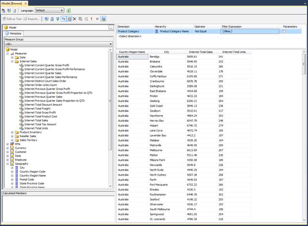
Figure 1: Browsing tabular data in SSMS
Notice in Figure 1 that I also created a filter that limits the amount of data returned. (You define filters in the small windows above the main workspace.) In this case, I eliminated all sales that include the value Bikes in the Category Name column of the Product table. This way, all non-bike merchandise is included in the sales figures.
What’s shown in Figure 1 is pretty much the extent of what you can do in the Browse window in SSMS. To be able to fully drill into the data, you need to use Excel. Starting with SQL Server 2012, Excel is now the de facto tool in SSMS and SSDT for analyzing tabular data. Unfortunately, that means you need Office 2003 or later installed on the same computer where SSMS and SSDT are installed, not a practical solution for everyone. Even so, having Excel installed makes analyzing tabular data a much easier process.
Part of that simplicity lies in the fact that the SSMS Browse window and the SSDT tabular project window both include the Analyze in Excel button on their respective menus. The button launches Excel and let’s you browse the tabular data from within in a pivot table.
When you first click the Analyze in Excel button, you must choose which perspective to open in Excel, as shown in Figure 2. As you might recall from the first article, a perspective represents all or part of the data model. The Model perspective includes all database components.
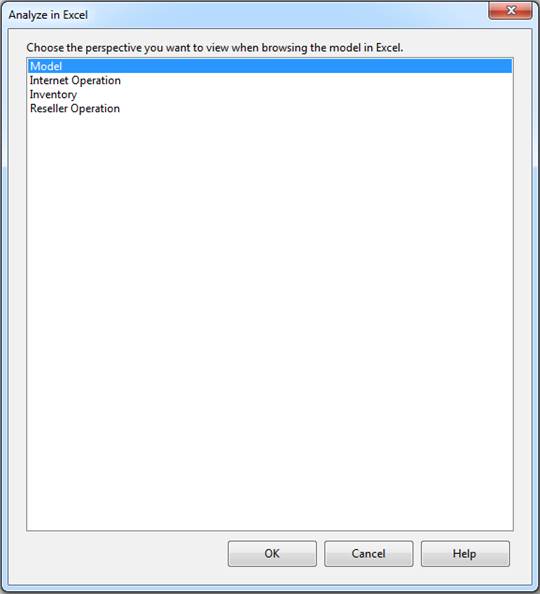
Figure 2: Selecting a perspective when sending data to Excel
Once you’ve selected a perspective, click OK. Excel is launched and opens to a new pivot table that automatically connects to the SSAS tabular data source. Figure 3 shows the pivot table before any data has been added. Notice in the right window you’ll find the PivotTable Field List pane, which contains a list of all your database objects, including tables, columns, and measures.
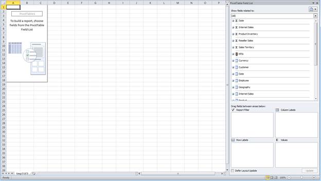
Figure 3: Importing tabular data into an Excel pivot table
To get started with the pivot table, drag the fields and measures you want to include in your report to the Column Labels, Row Labels, and Values panes. The data will then be displayed in the pivot table. You can also create filters by dragging fields to the Report Filter pane. Figure 4 shows the pivot table after I added numerous database objects. Many of these objects are the same columns and measures that were added to the Browse window shown in Figure 1, except that now I also break down the sales by years.
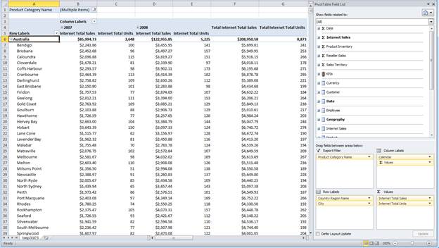
Figure 4: Working with tabular data in an Excel pivot table
To configure the pivot table shown in Figure 4, I added the following database objects to the specified configuration panes in the right window:
- The
Country Region Namecolumn from theGeographytable to theRow Labelspane. - The
Citycolumn from theGeographytable to theRow Labelspane. - The
Yearcolumn (from the Calendar hierarchy) of theDatetable to theColumn Labelspane. - The
Internet Total Salesmeasure from the Internet Salestable to theValuespane. - The
Internet Total Unitsmeasure from theInternet Salestable to theValuespane. - The
Product Category Namecolumn from theProducttable to theReport Filterpane.
Once you’ve set up your pivot table, you can play around with the data however you want. For example, you can drill down into the year values or view only the country totals without viewing the cities. You can also find rollups for each category of data. Plus, you can filter data based on the values in the Product Category Name column. Keep in mind, however, that this article is by no means a tutorial on how to work with Excel pivot tables. For that, you need to check out the Excel documentation. SSMS and SSDT make it easy to view the data in Excel, but it’s up to you to derive meaning from what you find.
Importing Data into an Excel Pivot Table
Not everyone will have SSMS or SSDT installed on their systems, but they might still need to access an SSAS instance to retrieve tabular data. In that case, they can establish their own connection to the tabular database (assuming they have the necessary permissions) and import the data into a pivot table, just as we saw above.
To connect to a tabular database from within Excel, go to the Data tab, click the From Other Sources button, and then click From Analysis Services. When the Data Connection Wizard appears, type the instance name and any necessary logon credentials, as shown in Figure 5. (In my case, I used Windows Authentication.)
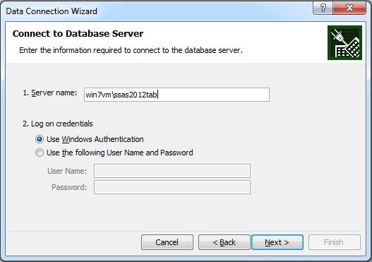
Figure 5: Connecting to an SSAS instance in tabular mode
Click Next to advance to the Select Database and Table page, shown in Figure 6. Here you select the database you want to connect to and the specific perspective. Once again, I’ve selected Model in order to retrieve all the database components. (As you’ve probably noticed, Microsoft is somewhat inconsistent in its interfaces when it comes to referring to perspectives in a tabular database. Sometimes they’re referred to as cubes, sometimes perspective, and sometimes Model is referred to as a cube and the other components as perspectives. I’m not sure how Table fits into the picture.)
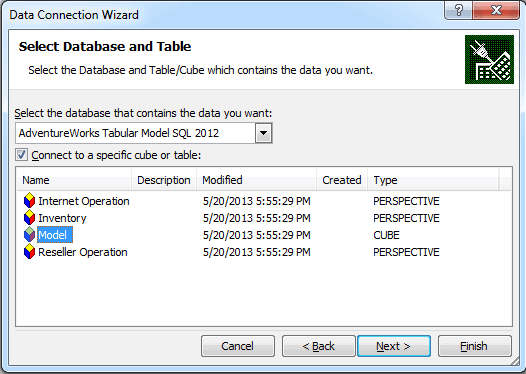
Figure 6: Selecting a perspective when connecting to tabular data
After you’ve selected your database and perspective, click Next to advance to the Save Data Connection File and Finish page, shown in Figure 7. Here you can provide a name for the data connection file (an .odc file), a description of the connection, and a friendly name for the connection.
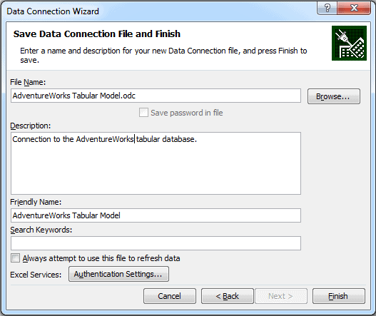
Figure 7: Creating a data connection file in Excel
Once you’ve supplied the necessary information, click Finish. You’ll then be presented with the Import Data dialog box, as shown in Figure 8. You can choose whether to create a pivot table, a pivot table and pivot chart, or the data connection only. You can also choose to use the existing worksheet or open a new one.
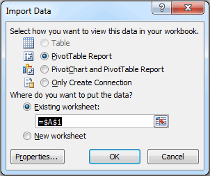
Figure 8: Importing tabular data into a pivot table
You might have noticed that the Table option is grayed out. When importing tabular data in this way, Excel is very picky. Either you use a pivot table (and pivot chart, if you want) or nothing at all. You cannot import the data into a set of tables. However, there is a way to work around the default behavior, which we cover in the following section.
But for now, stick with the default options (those shown in Figure 8), and click OK. You’ll then be presented with a new pivot table and the PivotTable Field List pane, with all the tables and their columns and measures listed, similar to what is shown in Figure 3. You can then work with that data to create a report just like we did earlier.
Using DAX to Import Data into Excel
To import tabular data into a regular Excel table, rather than a pivot table, we can create a DAX expression that pulls in exactly the data we need. We start by creating a data connection, just as we did in the last section. Once again, launch the Data Connection Wizard and follow the prompts. When you get to the Save Data Connection File and Finish page, provide a file name, description, and friendly name. But keep all the names simple because we’ll be referencing them later in the process and we want to make sure everything is easy to find. Figure 9 shows the names I used to set up the data connection on my system.
Figure 9: Creating a data connection file in Excel
When you click Finish, you’ll again be presented with the Import Data dialog box. This time around, select the option Only Create Connection, as shown in Figure 10. We don’t want to pull in any data just yet. We just want to establish how we’ll be connecting to the tabular database. Click OK to finish creating the connection.
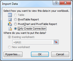
Figure 10: Creating a data connection without creating a pivot table
The next step is to locate the data connection file we just created so we can edit it. On my system, I had named the file aw_query.odc, and I found it in the My Documents/My Data Sources folder associated with my user account.
When editing the connection file, which we can do in Notepad, we want to modify the default settings so we can use a DAX query to retrieve the data. To achieve this, we need to modify two lines, the CommandType and CommandText elements, which are highlighted in the following HTML:
|
1 2 3 4 5 6 7 8 9 10 11 12 13 14 15 16 17 18 19 20 21 22 23 24 25 26 27 28 29 30 31 32 33 |
<head> <meta http—equiv=Content—Type content=«text/x—ms—odc; charset=utf—8«> <meta id=«ProgId« content=ODC.Cube> <meta id=«SourceType« content=OLEDB> <meta id=«Catalog« content=«AdventureWorks Tabular Model SQL 2012«> <meta id=«Table« content=Model> <title>AdventureWorks query</title> <xml id=«docprops><o:DocumentProperties«> xmlns:o=«urn:schemas—microsoft—com:office:office« xmlns=«http://www.w3.org/TR/REC—html40«> <o:Description>Generate DAX statement to retrieve table from AdventureWorks database.</o:Description> <o:Name>AdventureWorks query</o:Name> </o:DocumentProperties> </xml> <xml id=«msodc><odc:OfficeDataConnection«> xmlns:odc=«urn:schemas—microsoft—com:office:odc« xmlns=«http://www.w3.org/TR/REC—html40«> <odc:Connection odc:Type=«OLEDB«> <odc:ConnectionString>Provider=MSOLAP.4;Integrated Security=SSPI;Persist Security Info=True;Data Source=win7vmssas2012tab;Initial Catalog=AdventureWorks Tabular Model SQL 2012</odc:ConnectionString> <odc:CommandType>Cube</odc:CommandType> <odc:CommandText>Model</odc:CommandText> </odc:Connection> </odc:OfficeDataConnection> </xml> <style> <!— .ODCDataSource { behavior: url(dataconn.htc); } —> </style> </head> |
The HTML shown here is the head section of the data connection file. For the CommandType element, replace the value Cube with the value query. This tells Excel to let us pass a query in through our data connection, rather than having to identify a specific perspective.
For the CommandText element, replace the value Model with a DAX statement that retrieves data into a single result set. For this example, I pulled the following query from the last article in this series (so return to that article for an explanation):
|
1 2 3 4 5 6 7 8 9 10 11 12 13 14 15 16 17 18 19 20 21 22 23 |
evaluate ( filter ( addcolumns ( summarize ( ‘Internet Sales’, ‘Product’[Product Name], ‘Product Subcategory’[Product Subcategory Name], ‘Product Category’[Product Category Name], ‘Date’[Calendar Year] ), «Total Sales Amount«, calculate(sum(‘Internet Sales’[Sales Amount])), «Total Cost«, calculate(sum(‘Internet Sales’[Total Product Cost])) ), ‘Date’[Calendar Year] > 2006 ) ) order by ‘Product’[Product Name], ‘Date’[Calendar Year] |
You can use a different query, of course, whatever serves your needs. The goal is to retrieve the data into a single table that you can view in an Excel worksheet, just like any other worksheet. After you modify the HTML in the data connection file, the head section should look similar to the following:
|
1 2 3 4 5 6 7 8 9 10 11 12 13 14 15 16 17 18 19 20 21 22 23 24 25 26 27 28 29 30 31 32 33 34 35 36 37 38 39 40 41 42 43 44 45 46 47 48 49 50 51 52 53 54 55 56 57 |
<head> <meta http—equiv=Content—Type content=«text/x—ms—odc; charset=utf—8«> <meta id=«ProgId« content=ODC.Cube> <meta id=«SourceType« content=OLEDB> <meta id=«Catalog« content=«AdventureWorks Tabular Model SQL 2012«> <meta id=«Table« content=Model> <title>AdventureWorks query</title> <xml id=«docprops><o:DocumentProperties«> xmlns:o=«urn:schemas—microsoft—com:office:office« xmlns=«http://www.w3.org/TR/REC—html40«> <o:Description>Generate DAX statement to retrieve table from AdventureWorks database.</o:Description> <o:Name>AdventureWorks query</o:Name> </o:DocumentProperties> </xml> <xml id=«msodc><odc:OfficeDataConnection«> xmlns:odc=«urn:schemas—microsoft—com:office:odc« xmlns=«http://www.w3.org/TR/REC—html40«> <odc:Connection odc:Type=«OLEDB«> <odc:ConnectionString>Provider=MSOLAP.4;Integrated Security=SSPI;Persist Security Info=True;Data Source=win7vmssas2012tab;Initial Catalog=AdventureWorks Tabular Model SQL 2012</odc:ConnectionString> <odc:CommandType>query</odc:CommandType> <odc:CommandText> evaluate ( filter ( addcolumns ( summarize ( ‘Internet Sales’, ‘Product’[Product Name], ‘Product Subcategory’[Product Subcategory Name], ‘Product Category’[Product Category Name], ‘Date’[Calendar Year] ), «Total Sales Amount«, calculate(sum(‘Internet Sales’[Sales Amount])), «Total Cost«, calculate(sum(‘Internet Sales’[Total Product Cost])) ), ‘Date’[Calendar Year] > 2006 ) ) order by ‘Product’[Product Name], ‘Date’[Calendar Year] </odc:CommandText> </odc:Connection> </odc:OfficeDataConnection> </xml> <style> <!— .ODCDataSource { behavior: url(dataconn.htc); } —> </style> </head> |
I highlighted the new code to make it easier to pick out. I also laid out the DAX statement so it’s more readable. However, you don’t need to break it apart in this way to add it into the file. (The parser ignores the extra whitespace and line breaks.)
After you save and close the data connection file, it’s time to verify what you’ve done. In Excel, go to the Data tab and click Existing Connections. When the Existing Connections dialog box appears, double-click the connection you just edited. It will be listed under its friendly name, not the file name. On my system, the connection’s friendly name is AdventureWorks query. This launches the Import Data dialog box, shown in Figure 11. Notice that this time around, the Table option is available and selected.
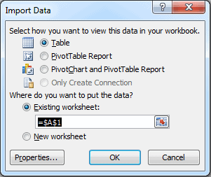
Figure 11: Importing tabular data into an Excel table
Click OK to close the Import Data dialog box. A table will appear, populated with the data retrieved through the DAX statement, as shown in Figure 11. You can then sort through the data and create any necessary filters.
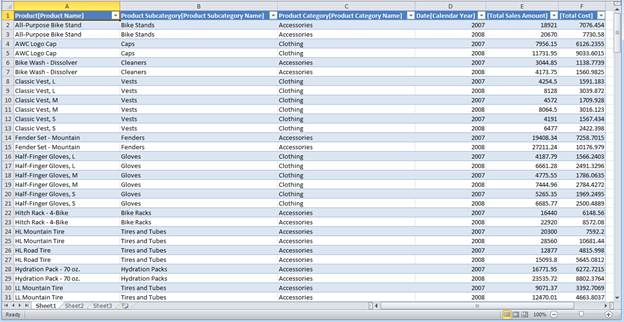
Figure 12: Working with tabular data in an Excel table
When you’re working in a table based on tabular data, you can modify the connection associated with the current workbook. Doing so, however, severs its relationship to the original .odc data connection file. Instead, your changes are saved to the connection specifically associated with that workbook. The .odc file remains unchanged. Updating the connection in this way lets you modify the DAX statement, change the connection string, or configure other properties.
To modify the workbook’s connection, go to the Data tab and click Connections. This launches the Workbook Connections dialog box, shown in Figure 13. Here you should find the connection you created earlier. On my system, this is AdventureWorks query.
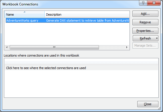
Figure 13: Viewing the data connections associated with an Excel workbook
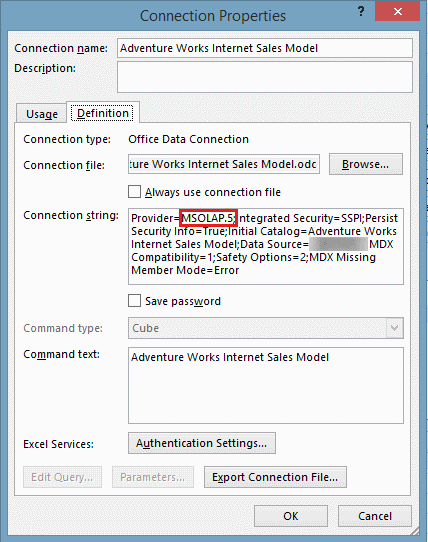
Next, we want to access the connection’s properties. Make sure the connection is selected (in case you have more than one connection listed), and then click Properties. This launches the Connection Properties dialog box. Go to the Definition tab and expand the dialog box as necessary to easily view the DAX statement. Figure 14 shows what the dialog box looks like on my system.
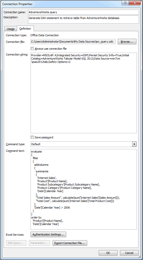
Figure 14: Viewing the properties of an Excel data connection
Chances are, when you open the dialog box, the DAX statement will be difficult to read. The statement shown in Figure 14 is what it looked like after I organized things a bit for readability. The changes I made have no impact on the statement itself.
You can modify the DAX statement or connection string as necessary (or any other properties, for that matter). To save you changes, click OK. You’ll then be presented with an Excel message box warning you that you are about to sever ties with the original data connection file, as shown in Figure 15. That’s not a problem, though, because your updated connection information will be saved with the workbook when you save it.
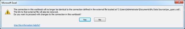
Figure 15: Severing ties between a data connection and its source file
You can now update you connection as often as you like. You should not receive this warning going forward. You can also use the existing .odc connection to easily add other tables to your workbook. To do so, add a new worksheet, connect to the data source via the .odc connection, and then modify the connection properties by adding a different DAX statement. (You can also rename the connection as necessary.) That way you can create a workbook that contains numerous worksheets that each includes an imported table from a tabular data source.
Using DAX to Import Data into PowerPivot
Up to this point, I’ve shied away from discussing PowerPivot in too great of detail, mostly because it’s already received so much press. But one issue that’s received little attention is how you retrieve data from an SSAS tabular instance into PowerPivot.
Surprisingly, the functionality is somewhat limited. You would expect-or at least I would expect-that I could import all the tables, along with their columns and measures, in a single connection, just as I can do with an Excel pivot table or a SQL Server database in PowerPivot. But that doesn’t appear to be the case. The only option I can find for importing tabular data directly into PowerPivot is one table at a time, just like we saw with Excel tables. However, doing so in PowerPivot is a bit easier.
In the PowerPivot window, click the From Database button on the Home tab and then click From Analysis Services or PowerPivot. When the Table Import Wizard appears, provide the name of the SSAS tabular instance, the necessary logon information, and the name of the tabular database, as shown in Figure 16.
Figure 16: Defining a data connection to an SSAS tabular database
Don’t forget, you can also provide a friendly connection name. And it’s always a good idea to test your connection. When you’re finished, click Next.
The next page in the wizard is Specify a MDX Query. As with SSMS or your Excel data connections, you can specify a DAX query rather than a Multidimensional Expressions (MDX) query. We’ll go with DAX. Figure 17 shows the page with the same query we used in the previous section. You can use the Validate option to check your statement, which seems to work with DAX, unlike the Design option, which seems happier sticking with MDX.
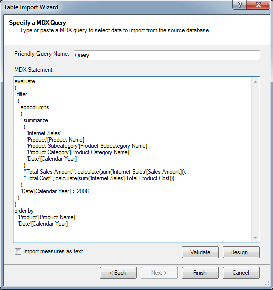
Figure 17: Defining a DAX query to retrieve tabular data from SSAS
After you entered your DAX query (and provided a name for the query, if you like), click Finish to import the data. During this process, you’ll advance to the wizard’s Importing page. If the data is imported with no problems, you should receive a Success message, as shown in Figure 18.
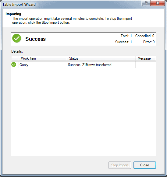
Figure 18: Successfully importing SSAS tabular data into PowerPivot for Excel
Click Close. This will open a new table in the PowerPivot window, with the imported data displayed. Figure 19 shows part of the data returned by the query. If the data is not exactly what you need, you can refine your query as necessary.
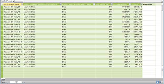
Figure 19: Working with tabular data in PowerPivot for Excel
You can import data into as many tables as you need. You can then create relationships between those tables, assuming you bring in the columns necessary to define those relationships. Not surprisingly, it would be handier to go directly to the source of the data, in this case, the AdventureWorksDW2012 database, so you can retrieve all the tables at once, along with their defined relationships. But you might not have access to that data and have no choice but to be retrieve it directly from the SSAS instance. Or there might be other circumstances that require you to retrieve the data directly from SSAS. Whatever the reason, you now know how it’s done, and once you’ve tried it out, you’ll find it’s a fairly simple operation.
The Excel Connection
As you’ve seen in this article, you have several options for retrieving SSAS tabular data into Excel. You can launch Excel from within SSMS or SSDT. You can import data directly into a pivot table. And you can generate DAX queries to retrieve data into individual Excel and PowerPivot tables. Or instead of DAX, you can generate MDX queries, unless the tabular database has been set up in DirectQuery mode. Regardless, you have a number of options for importing tabular data into Excel. And once you get it there, you have a rich environment for manipulating and analyzing the data, allowing you to create precise and detailed reports in the format you need when you need them, without having to be concerned about SSAS and how the tabular model works.
Содержание
- Анализ в Excel
- Предварительные требования
- Просмотр с помощью перспективы по умолчанию и перспективы Internet Sales
- Просмотр с использованием перспективы по умолчанию
- Просмотр с использованием перспективы Internet Sales
- Просмотр с помощью ролей
- Просмотр с помощью роли пользователя Sales Manager
- Следующий шаг
- Настройка поставщика данных MSOLAP для Excel для подключения к службам Analysis Services
- Аннотация
- Дополнительные сведения
- Подключение в SQL Server служб Analysis Services (импорт)
- Configure MSOLAP data provider for Excel to connect to Analysis Services
- Summary
- More information
Анализ в Excel
Применимо к:  SQL Server 2019 и более поздних версий analysis Services Azure Analysis Services Power BI Premium
В этом занятии вы воспользуетесь функцией «Анализ в Excel», чтобы открыть Microsoft Excel, автоматически создать подключение к рабочей области модели и автоматически добавить сводную таблицу на лист. Функция «Анализ в Excel» предназначена для быстрого и удобного тестирования эффективности модели до ее развертывания. В этом занятии выполнять анализ данных не нужно. Оно призвано познакомить вас как автора модели со средствами для проверки модели.
Для этого занятия нужно установить Excel на том же компьютере, где находится Visual Studio.
Предполагаемое время выполнения этого занятия: 5 минут.
Предварительные требования
Эта статья является одной из частей руководства по созданию табличных моделей. Эти части следует изучать в предложенном порядке. Прежде чем выполнять задачи в этом разделе, нужно завершить предыдущее занятие: Занятие 11. Создание ролей.
Просмотр с помощью перспективы по умолчанию и перспективы Internet Sales
В этих первых задачах вы просматриваете модель с помощью перспективы по умолчанию, которая включает все объекты модели, а также с помощью созданной ранее перспективы продаж в Интернете. Перспектива «Продажи через Интернет» исключает объект таблицы «Заказчик».
Просмотр с использованием перспективы по умолчанию
Щелкните ExtensionsModelAnalyze> >в Excel.
В диалоговом окне Анализ в Excel нажмите кнопку ОК.
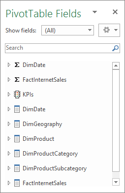
В Excel открывается новая книга. Создается соединение с источником данных, использующее учетную запись текущего пользователя, и перспектива по умолчанию используется для определения доступных для просмотра полей. На лист автоматически добавляется сводная таблица.
В Excel в списке полей сводной таблицы отображаются группы мер DimDate и FactInternetSales. Также отображаются следующие таблицы со связанными столбцами: DimCustomer, DimDate, DimGeography, DimProduct, DimProductCategory, DimProductSubcategory и FactInternetSales.
Закройте Excel, не сохраняя книгу.
Просмотр с использованием перспективы Internet Sales
Щелкните ExtensionsModelAnalyze> >в Excel.
В диалоговом окне Анализ в Excel оставьте выбранным вариант Текущий пользователь Windows , в раскрывающемся списке Перспектива выберите Продажи через Интернети нажмите кнопку ОК.
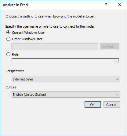
В области Поля сводной таблицы Excel обратите внимание на то, что таблица DimCustomer исключена из списка полей.
Закройте Excel, не сохраняя книгу.
Просмотр с помощью ролей
Роли — это неотъемлемая часть любой табличной модели. Если пользователям не назначить хотя бы одну роль, они не смогут использовать и анализировать данные с помощью вашей модели. Функция «Анализ в Excel» позволяет проверить создаваемые роли.
Просмотр с помощью роли пользователя Sales Manager
Щелкните ExtensionsModelAnalyze> >в Excel.
В поле Укажите имя пользователя или роль для подключения к модели щелкните Роль и выберите Менеджер по продажам в раскрывающемся списке. Затем нажмите кнопку ОК.
В Excel открывается новая книга. Автоматически создается сводная таблица. Список полей сводной таблицы включает все поля данных, доступные в новой модели.
Закройте Excel, не сохраняя книгу.
Следующий шаг
Перейдите к следующему занятию: занятие 13. Развертывание
Источник
Настройка поставщика данных MSOLAP для Excel для подключения к службам Analysis Services
В этой статье описывается настройка правильного поставщика данных MSOLAP для Excel для подключения к службам Analysis Services.
Исходная версия продукта: SQL Server 2017 Корпоративная, SQL Server 2016 Корпоративная, SQL Server 2014 Корпоративная, SQL Server 2012 Корпоративная, SQL Server 2008 Корпоративный
Исходный номер базы знаний: 4488253
Аннотация
Чтобы создать подключение к данным к источнику данных служб Analysis Services, Microsoft Excel использует поставщик OLE DB служб Microsoft Analysis Services для Microsoft SQL Server (MSOLAP). Каждая версия служб Analysis Services имеет собственную версию поставщика MSOLAP. В следующей таблице перечислены версии службы Analysis Services и их соответствующая версия поставщика MSOLAP.
| Версия служб Analysis Services | Версия поставщика MSOLAP |
|---|---|
| SQL Server 2008 | MSOLAP.4 |
| SQL Server 2012 | MSOLAP.5 |
| SQL Server 2014 | MSOLAP.6 |
| SQL Server 2016 | MSOLAP.7 |
| SQL Server 2017 и более поздних версий | MSOLAP.8 (считается evergreen) |
Дополнительные сведения о MSOLAP и других клиентских библиотеках для служб Analysis Services см. в клиентских библиотеках служб Analysis Services.
Дополнительные сведения об использовании правильной версии MSOLAP см. в свойствах строки подключения. Сведения о устаревших версиях MSOLAP см. в статье «Как получить последние версии MSOLAP». Последнюю версию MSOLAP см. в клиентских библиотеках служб Analysis Services.
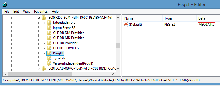
В Excel используется версия поставщика MSOLAP, установленная на клиентском устройстве. В следующем примере Excel настроит MSOLAP.5 в качестве поставщика данных в строке подключения к данным.
На клиентском устройстве, на котором установлено несколько версий поставщика MSOLAP, Excel использует версию, настроенную в реестре.
Например, в следующем сценарии:
- В реестре установлено и настроено приложение MSOLAP.5.
- Вы установили MSOLAP.6 на устройстве для подключения к Analysis Services 2014, но не обновили реестр для ссылки на MSOLAP.6.
Excel настроит подключение для использования MSOLAP.5 в строке подключения. Это вызывает проблемы, так как вы не можете использовать версии MSOLAP, предшествующие версии источника данных.
Дополнительные сведения
Чтобы указать версию MSOLAP, которую использует Excel, обновите версию в разделах реестра. Следующие ключи определяют, какую версию MSOLAP Excel использует для подключения к службам Analysis Services. Расположение раздела реестра зависит от того, является ли Microsoft Office установкой MSI или «нажми и запускай» (C2R), а также от того, является ли он 32-разрядным или 64-разрядным.
32-разрядная версия MSI Office
64-разрядная версия Office MSI
Office 32-разрядная версия C2R
Office 64-разрядная версия C2R
Ниже приведен пример 32-разрядной версии Office C2R, настроенной для использования MSOLAP.5:

Чтобы определить, является ли ваша установка MSI или C2R, в Excel перейдите к учетной записи файла>. Если вы видите раздел office Обновления, установка будет C2R:
Если раздел office Обновления, это установка MSI:
Чтобы определить, является ли Excel 32-разрядным или 64-разрядным, щелкните «О Программе Excel » на том же экране «Учетные записи», и в верхней части окна отобразится диалоговое окно:
Источник
Подключение в SQL Server служб Analysis Services (импорт)
Вы можете создать динамическое подключение между книгой Excel и сервером базы данных SQL Server Analysis Services Online Analytical Processing (OLAP ), а затем обновлять это подключение при внесении изменений. Вы можете подключиться к определенной автономный файл куба, если она создана на сервере базы данных. Вы можете импортировать данные в Excel как таблицу или отчет таблицы.
Используйте Excel Power Query (Получить & Transform( Power Query) для подключения к серверу базы данных SQL Server Analysis Services (OLAP ).
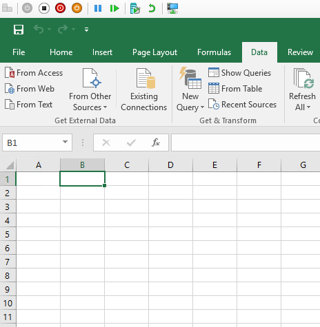
На вкладке Данные нажмите кнопку Получить данные > из базы > из базы SQL Server служб Analysis Services (Импорт). Если вы не видите кнопку Получить данные, нажмите кнопку Новый запрос > из базы данных > из базы данных analysis Services SQL Server.
Ввести имя сервера и нажмите кнопку ОК.
Примечание: Вы можете ввести имя конкретной базы данных, а также добавить запрос многоязовой или DAX.
В области Навигатор выберите базу данных, а затем куб или таблицы, которые вы хотите соединить.
Нажмите кнопку Загрузить, чтобы загрузить выбранную таблицу, или изменить, чтобы выполнить дополнительные фильтры и преобразования данных перед загрузкой.
В Excel 2010 и 2013 года существует два способа создания подключения к базе данных SQL Server analysis Services (OLAP). Рекомендуемый способ — использовать Power Query, который доступен при скачии надстройки Power Query. Если вы не можете скачать Power Query, воспользуйтесь мастером подключения к данным.
На ленте Power Query щелкните Из базы > Из SQL Server служб Analysis Services.
Ввести имя сервера и нажмите кнопку ОК.
Примечание: Вы можете ввести имя конкретной базы данных, а также добавить запрос многоязовой или DAX.
В области Навигатор выберите базу данных, а затем куб или таблицы, которые вы хотите соединить.
Нажмите кнопку Загрузить, чтобы загрузить выбранную таблицу, или изменить, чтобы выполнить дополнительные фильтры и преобразования данных перед загрузкой.
Мастер подключения к данным
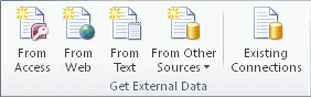
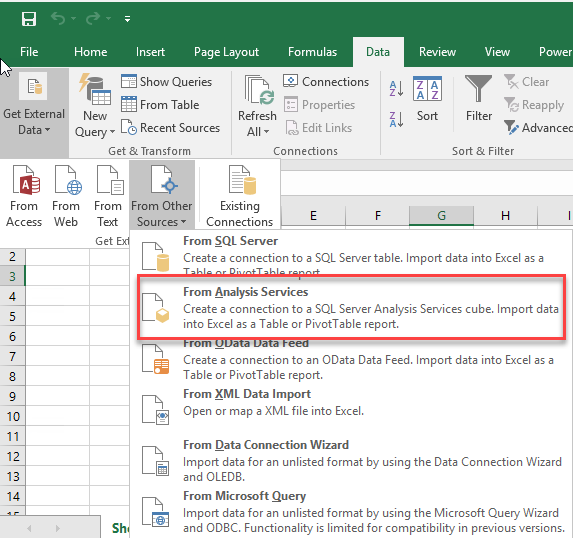
На вкладке Данные в группе Внешние данные нажмите кнопку Из других источников ивыберите из служб Analysis Services.
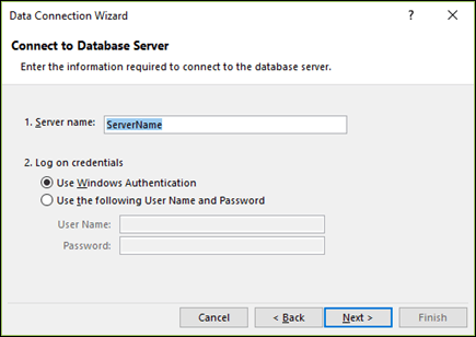
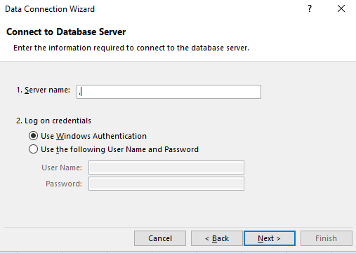
В мастере подключения к даннымвведите имя сервера и выберите параметр входа. Нажмите кнопку Далее.
 Подключение на сервер» loading=»lazy»>
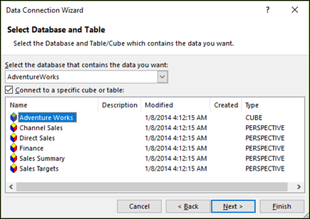
Выберите базу данных и таблицу или куб, к которой нужно подключиться, и нажмите кнопку Далее.
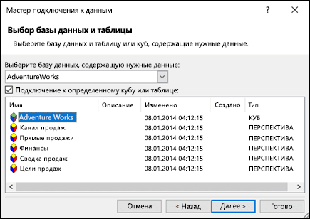 выберите базу данных и таблицу» loading=»lazy»>
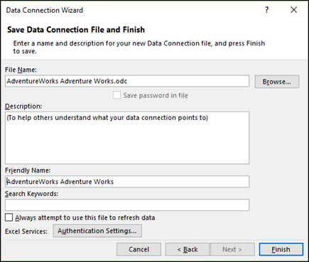
Введите имя и описание нового подключения и нажмите кнопку Готово, чтобы сохранить его.
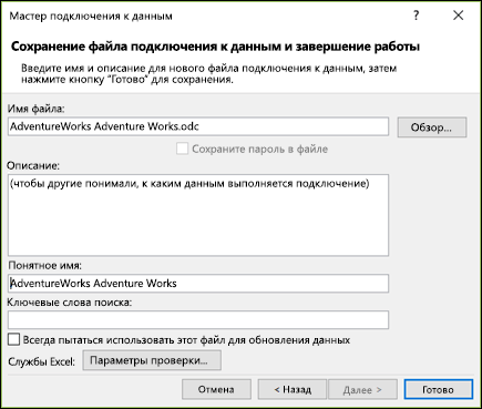 сохранить файл подключения к данным и завершить работу» loading=»lazy»>
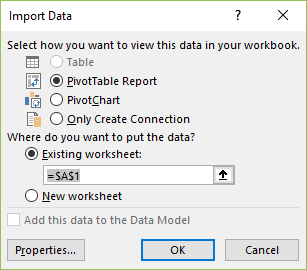
В диалоговом оке Импорт данных выберите способ и место извлечения данных. Начиная с Excel 2013 г., вы также можете сохранить данные в модели данных.
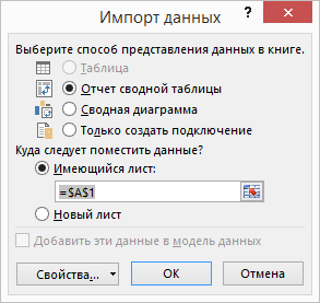 импорт данных» loading=»lazy»>
Источник
Configure MSOLAP data provider for Excel to connect to Analysis Services
This article describes how to configure the correct MSOLAP data provider for Excel to connect to Analysis Services.
Original product version: В SQL Server 2017 Enterprise, SQL Server 2016 Enterprise, SQL Server 2014 Enterprise, SQL Server 2012 Enterprise, SQL Server 2008 Enterprise
Original KB number: В 4488253
Summary
To create a data connection to an Analysis Services data source, Microsoft Excel uses the Microsoft Analysis Services OLE DB Provider for Microsoft SQL Server (MSOLAP). Each version of Analysis Services has its own MSOLAP provider version. The following table lists the Analysis Service versions and their corresponding MSOLAP provider version.
| Analysis Services version | MSOLAP provider version |
|---|---|
| SQL Server 2008 | MSOLAP.4 |
| SQL Server 2012 | MSOLAP.5 |
| SQL Server 2014 | MSOLAP.6 |
| SQL Server 2016 | MSOLAP.7 |
| SQL Server 2017 and later versions | MSOLAP.8 (Considered evergreen) |
For more information about MSOLAP and other client libraries for Analysis Services, review Analysis Services client libraries.
For more information about how to use the correct version of MSOLAP, see Connection string properties. For legacy MSOLAP versions, please refer to How to obtain the latest versions of MSOLAP. For latest MSOLAP version, please refer to Analysis Services client libraries.
Excel uses the version of the MSOLAP provider that is installed on the client device. In the following example, Excel has configured MSOLAP.5 as the data provider in the data connection string.

On a client device that has multiple versions of the MSOLAP provider installed, Excel uses the version that’s configured in the registry.
For example, in the following scenario:
- You have MSOLAP.5 installed and configured in the registry.
- You have installed MSOLAP.6 on your device to connect to Analysis Services 2014, but you have not updated the registry to reference MSOLAP.6.
Excel will configure the connection to use MSOLAP.5 in the connection string. This causes issues as you cannot use MSOLAP versions that are earlier than the data source version.
More information
To specify the version of MSOLAP that Excel uses, update the version in the registry keys. The following keys define which MSOLAP version Excel uses to connect to Analysis Services. The location of the registry key depends on whether Microsoft Office is an MSI or Click-to-Run (C2R) installation, and whether it’s 32-bit or 64-bit.
Office 32-bit MSI
Office 64-bit MSI
Office 32-bit C2R
Office 64-bit C2R
The following is an example of Office 32-bit C2R configured to use MSOLAP.5:
To determine whether your installation is MSI or C2R, in Excel go to File > Account. If you see an Office Updates section, the installation is C2R:

If there’s no Office Updates section, then it’s an MSI installation:

To determine whether Excel is 32-bit or 64-bit, click About Excel in the same Accounts screen and it will show you in the dialog box at the top:
Источник
1. Получаем разрешение на доступ к OLAP-кубу SQL Server Analysis Services (SSAS)
2. На вашем компьютере должен быть установлен MS Excel 2016 / 2013 / 2010 (можно и MS Excel 2007, но в нем работать не удобно, и совсем бедная функциональность MS Excel 2003)
3. Открываем MS Excel, запускаем мастер настройки соединения с аналитической службой:

3.1 Указываем имя или IP-адрес действующего сервера OLAP (иногда требуется указать номер открытого порта, например, 192.25.25.102:80); используется доменная аутентификация:

3.2 Выбираем многомерную базу данных и аналитический куб (в случае наличия прав доступа к кубу):

3.3 Настройки соединения с аналитической службой будут сохранены в odc-файле на Вашем компьютере:

3.4 Выбираем вид отчета (сводная таблица/график) и указываем место для его размещения:

Если в книге Excel уже создано подключение, то им можно воспользоваться повторно: главное меню «Данные» -> «Существующие подключения» -> выбираем подключение в этой книге -> вставляем сводную таблицу в указанную ячейку.
4. Успешно подключились к кубу, можно приступать к интерактивному анализу данных:

Приступая к интерактивному анализу данных необходимо определить, какие из полей будут участвовать в формировании строк, столбцов и фильтров (страниц) сводной таблицы. В общем случае сводная таблица является трехмерной, и можно считать, что третье измерение расположено перпендикулярно экрану, а мы наблюдаем сечения, параллельные плоскости экрана и определяемые тем, какая «страница» выбрана для отображения. Фильтрацию можно осуществить путем перетаскивания мышью соответствующих атрибутов измерений в область фильтров отчета. Фильтрация ограничивает пространство куба, уменьшая нагрузку на сервер OLAP, поэтому предпочтительнее в первую очередь установить необходимые фильтры. Затем следует размещать атрибуты измерений в областях строк, столбцов и показатели в область данных сводной таблицы.
Каждый раз, когда изменяется сводная таблица, на сервер OLAP автоматически отправляется MDX-инструкция, по исполнении которой возвращаются данные. Чем больше и сложнее объем обрабатываемых данных, рассчитываемых показателей, тем дольше время исполнения запроса. Отменить исполнение запроса можно нажатием клавиши Escape. Последние выполненные операции можно отменить (Ctrl+Z) или вернуть (Ctrl+Y).
Как правило, для наиболее часто используемых сочетаний атрибутов измерений в кубе хранятся заранее рассчитанные агрегированные данные, поэтому время отклика таких запросов несколько секунд. Однако все возможное комбинации агрегаций просчитать невозможно, так как для этого может потребоваться очень много времени и места для хранения. Для исполнения массивных запросов к данным на уровне детализации могут потребоваться значительные вычислительные ресурсы сервера, поэтому время их исполнения может быть продолжительным. После чтения данных с дисковых накопителей сервер помещает их в кэш оперативной памяти, что позволяет последующим таким запросам выполняться мгновенно, поскольку данные будут извлекаться уже из кэша.
Если Вы считаете, что ваш запрос будет часто использоваться и время его исполнения неудовлетворительно, Вы можете обратиться в службу сопровождения аналитических разработок для оптимизации выполнения запроса.
После размещения иерархии в области строк / столбцов возможно скрыть отдельные уровни:

У ключевых атрибутов (реже — для атрибутов выше по иерархии) измерений могут быть свойства — описательные характеристики, которые могут отображаться как во всплывающих подсказках, так и в виде полей:

Если требуется отобразить сразу несколько свойств полей, то можно воспользоваться соответствующим диалоговым списком:

Определяемые пользователем наборы
В Excel 2010 появилась возможность интерактивного создания собственных (определяемых пользователем) наборов из элементов измерения:

В отличие от наборов создаваемых и хранящихся централизованно на стороне куба, пользовательские наборы сохраняются локально в книге Excel и могут использоваться в дальнейшем:

Продвинутые пользователи могут создавать наборы, используя MDX конструкции:

Настройка свойств сводной таблицы
Посредством пункта «Параметры сводной таблицы…» контекстного меню (щелчок правой кнопкой мыши в рамках сводной таблицы) предоставляется возможность настройки сводной таблицы, например:
— вкладка «Вывод», параметр «Классический макет сводной таблицы» — сводная таблица становится интерактивной, можно перетаскивать поля (Drag&Drop);
— вкладка «Вывод», параметр «Показывать элементы без данных в строках» — в сводной таблице будут отображаться пустые строки, не содержащие ни одного значения показателя по соответствующим элементам измерений;
— вкладка «Разметка и формат», параметр «Сохранять форматирование ячеек при обновлении» — в сводной таблице можно переопределить и сохранить формат ячеек при обновлении данных;

Создание сводных диаграмм
Для имеющейся сводной OLAP-таблицы можно создать сводную диаграмму – круговую, линейчатую, гистограмму, график, точечную и другие виды диаграмм:

При этом сводная диаграмма будет синхронизирована со сводной таблицей – при изменении состава показателей, фильтров, измерений в сводной таблице также обновляется сводная таблица.
Создание информационных панелей
Выделим исходную сводную таблицу, скопируем ее в буфер обмена (Ctrl+C) и вставим её копию (Ctrl+V), в которой изменим состав показателей:

Для одновременного управления несколькими сводными таблицами вставим срез (новый функционал, доступный, начиная с версии MS Excel 2010). Подключим наш Slicer к сводным таблицам – щелчок правой кнопкой мыши в рамках среза, выбор в контекстном меню пункта «Подключения к сводной таблице…». Следует отметить, что может быть несколько панелей срезов, которые могут обслуживать одновременно сводные таблицы на разных листах, что позволяет создавать скоординированные информационные панели (Dashboard).
 в сводную таблицу OLAP")
Панели срезов можно настраивать: необходимо выделить панель, затем см. пункты «Размер и свойства…», «Настройки среза», «Назначить макрос» в контекстном меню, активируемого по правому щелку мыши или пункт «Параметры» главного меню. Так, возможно установить кличество столбцов для элементов (кнопок) среза, размеры кнопок среза и панели, определить для среза цветовую гамму и стиль оформления из имеющегося набора (или создать свой стиль), определить собственный заголовок панели, назначить программный макрос, посредством которого можно расширить функционал панели.

Исполнение MDX запроса из Excel
- Прежде всего, необходимо выполнить операцию DRILLTHROUGH на каком-нибудь показателе, т.е. спуститься к детализированным данным (детализированные данные отображаются на отдельном листе), и открыть список подключений;
- Открыть свойства подключения, перейти на вкладку «Определение»;
- Выбрать тип команды по умолчанию, а в поле текста команды разместить заранее подготовленный MDX запрос;
- При нажатии кнопки после проверки правильности синтаксиса запроса и наличия соответствующих прав доступа запрос исполнится на сервере, а результат будет представлен в текущем листе в виде обычной плоской таблицы.
Посмотреть текст MDX-запроса, генерируемого Excel, можно с помощью установки бесплатного дополнения OLAP PivotTable Extensions, которое предоставляет также и другие дополнительные функциональные возможности.

Перевод на другие языки
Аналитический куб поддерживает локализацию на русский и английский языки (при необходимости возможна локализация на другие языки). Переводы распространяются на наименования измерений, иерархий, атрибутов, папок, мер, а также элементы отдельных иерархий в случае наличия для них переводов на стороне учетных систем/ хранилища данных. Чтобы сменить язык, необходимо открыть свойства подключения и в строке подключения добавить следующую опцию:
Extended Properties=»Locale=1033″
где 1033 — локализация на английский язык
1049 — локализация на русский язык

Дополнительные расширения Excel для Microsoft OLAP
Возможности работы с OLAP-кубами Microsoft возрастут, если использовать дополнительные расширения, например, OLAP PivotTable Extensions, благодаря которому можно пользоваться быстрым поиском по измерению:

![]()
dvbi.ru
2011-01-11 16:57:00Z
Последнее изменение: 2021-12-12 22:27:25Z
Возрастная аудитория: 14-70
Комментариев: 0