
Create a Spreadsheet in Excel (Table of Content)
- Introduction to Create Spreadsheet in Excel
- How to Create a Spreadsheet in Excel?
Introduction to Create Spreadsheet in Excel
A spreadsheet is a grid-based file designed to manage or perform any calculation on personal or business data. It is the best choice for users because it has 400+ functions and features such as pivot, coloring, graph, chart, and conditional formatting. It is accessible in both Office 365 and MS Office. Office 365 is a cloud-based application, whereas MS Office is an on-premises solution.
The workbook is the Excel lingo for ‘spreadsheet.’ MS Excel uses this term to emphasize that a single workbook can contain multiple worksheets, each with its own data grid, chart, or graph.
How to Create a Spreadsheet in Excel?
Here are a few examples of creating different types of spreadsheets in Excel with the key features of the created spreadsheets.
You can download this Create Spreadsheet Excel Template here – Create Spreadsheet Excel Template
Example #1 – How to Create Spreadsheet in Excel?
Step 1: Open MS Excel.
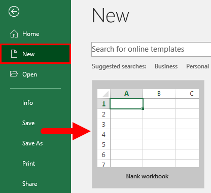
Step 2: Go to Menu and select New >> Click on the Blank workbook to create a simple worksheet.
OR – Press Ctrl + N: To create a new spreadsheet.
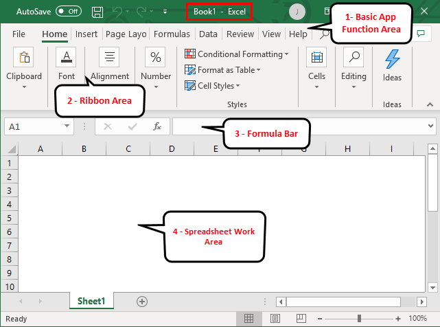
Step 3: By default, Sheet 1 will be created as a worksheet in the spreadsheet. The name of the spreadsheet will be given as Book 1 if you are opening it for the first time.
Key Features of the Created Spreadsheet:
- Basic App Functions Area: There is a green banner that contains all types of actions to perform on the worksheet, like – save the file, back or front step move, new, undo, redo, and many more.
- Ribbon Area: This is a gray area just below the basic app functions area called Ribbon. It contains data manipulation, a data visualizing toolbar, page layout tools, and many more.
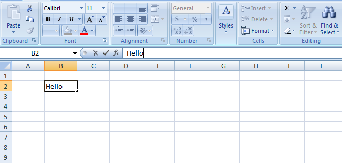
- Spreadsheet Work Area: By default, a grid contains alphabetic columns like A, B, C, …, Z, ZA…, ZZ, ZZA… and rows as numbers like 1,2 3, …. 100, 101, and… so on. Each rectangle box in the spreadsheet is called a cell, like the one selected in the above image (cell A1). It is a cell where the user can perform their calculation for personal or business data.
- Formula Bar: It shows the data in the selected cell; if it contains any formula, it will show here. Like the above area, a search bar is available in the top right corner, and a sheet tab is available on the downside of the worksheet. A user can change the name of the sheet name.
Once you create an Excel Spreadsheet, you can convert it to a universally accepted format like PDF. For convenience, some useful Excel to PDF converters converts Excel to PDF files for free while maintaining the original formatting.
Example #2 – How to Create a Simple Budget Spreadsheet in Excel?
Suppose a user wishes to design a spreadsheet for budget calculation. For 2018, he has a few products and their quarterly sales. He now wants to present his client with this budget.
Let’s see how we can do this with the help of the spreadsheet.
Step 1: Open MS Excel.
Step 2: Go to Menu and select New >> Click on the Blank workbook to create a simple worksheet.
OR – Press Ctrl + N: To create a new spreadsheet.

Step 3: Go to the spreadsheet work area, sheet 1.
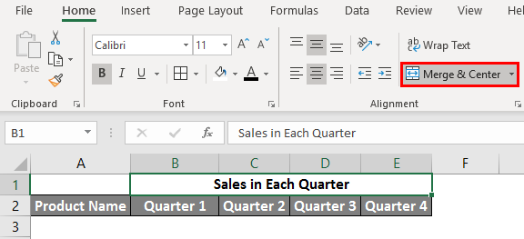
Step 4: Now create headers for Sales in each quarter in the first row by merging cells from B1 to E1. In row 2, give the product name and each quarter’s name.
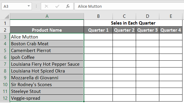
Step 5: Write down all product names in column A.
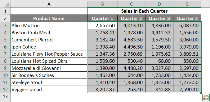
Step 6: Provide the sales data for each quarter before every product.
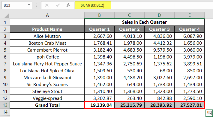
Step 7: In the next row, put one header for Grand Total and calculate each quarter’s total sales.
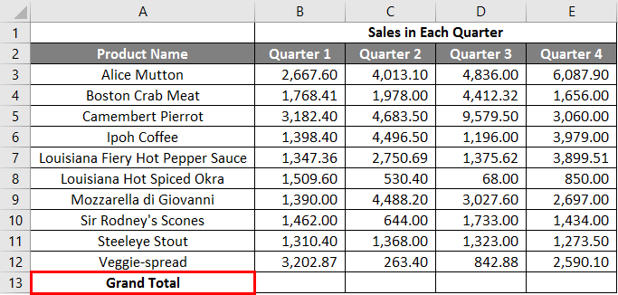
Step 8: Calculate the grand total for each quarter by summation >> apply in other cells in B13 to E13.
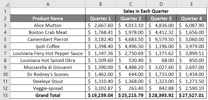
Step 9: Let’s convert the sales value into the ($) currency symbol.
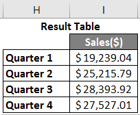
Step 10: Create a Result Table with each quarter’s total sales.
Plot the pie chart to represent the data to the client in a professional way that looks attractive. A user can change the look of the graph by just clicking on it.
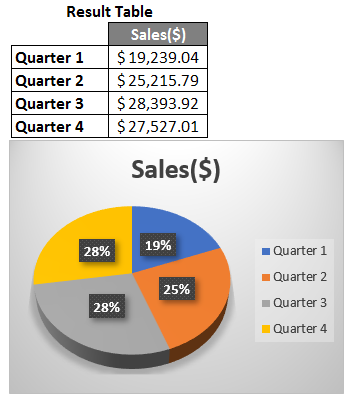
Summary of Example 2: As the user wants to create a spreadsheet to represent sales data to the client, it is done here.
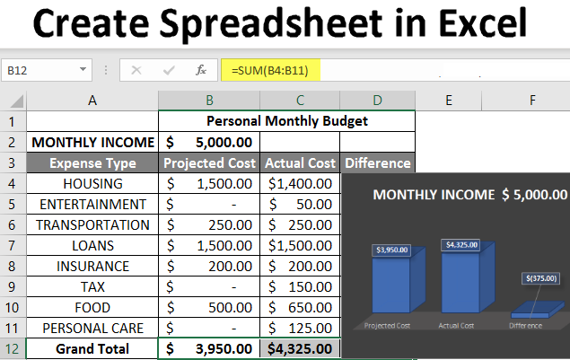
Example #3 – How to Create a Personal Monthly Budget Spreadsheet in Excel?
Let’s assume a user wants to create a spreadsheet to determine their monthly personal budget. For the year 2022, he has estimated costs and actual costs. He now wants to show his family this budget.
Let’s see how we can do this with the help of the spreadsheet.
Step 1: Open MS Excel.
Step 2: Go to Menu and select New >> Click on the Blank workbook to create a simple worksheet.
OR – Press Ctrl + N: To create a new spreadsheet.

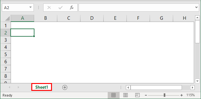
Step 3: Go to the spreadsheet work area, Sheet 2.
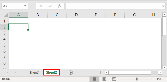
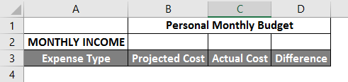
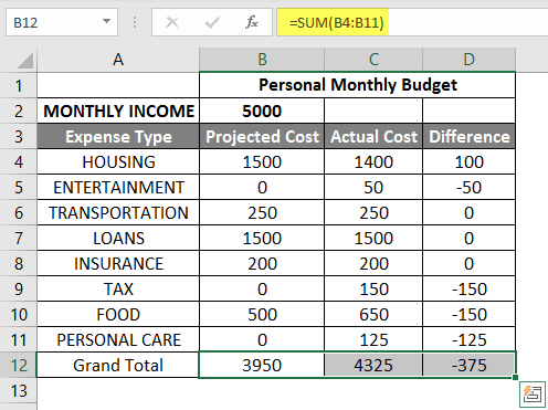
Step 4: Now create headers for Personal Monthly Budget in the first row by merging cells from B1 to D1. In row 2, give MONTHLY INCOME; in row 3, give Expense type, Projected Cost, Actual Cost, and Difference.
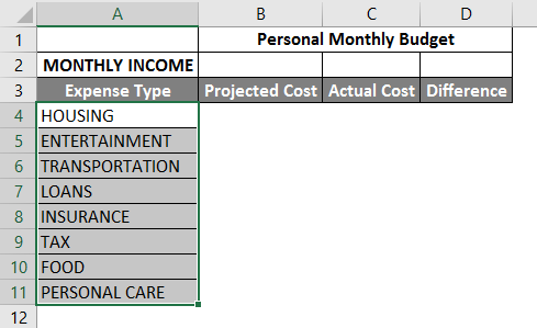
Step 5: Write down all the expenses in column A.
Step 6: Now, provide the monthly income, Projected cost, and Actual Cost data for each expense type.
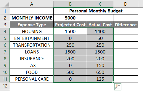
Step 7: In the next row, put one header for Grand Total and calculate the total and difference from the project to the actual cost.
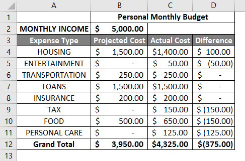
Step 8: Now highlight the header and add boundaries using toolbar graphics. >> The cost and income value in $, so make it by currency symbol.
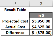
Step 9: Create a Result Table with each quarter’s total sales.
Step 10: Plot the pie chart to represent the data for the family. A user can choose one which he likes.
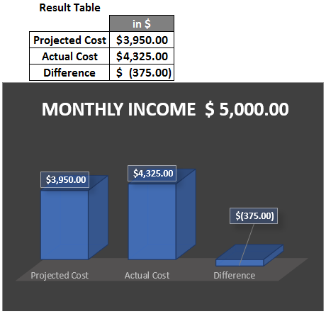
Summary of Example 3: As the user wanted to create a spreadsheet to represent monthly budget data to the family, we have created the same here. The close bracket shows in the data for the negative value.
Things to Remember
- A spreadsheet is a grid-based file designed to manage or perform any calculation on personal or business data.
- It is available in MS Office as well as Office 365.
- The workbook is the Excel lingo for ‘spreadsheet.’ MS Excel uses this term to emphasize that a single workbook can contain multiple worksheets.
How to add data in a spreadsheet Video
Recommended Articles
This article is a comprehensive guide to creating Spreadsheets in Excel. Here we have discussed how to create a Spreadsheet in Excel, examples, and a downloadable Excel template. You may also look at the following articles to learn more –
- Excel Spreadsheet Formulas
- Group Worksheets In Excel
- Excel Spreadsheet Examples
- Worksheets in Excel
Программа Microsoft Excel удобна для составления таблиц и произведения расчетов. Рабочая область – это множество ячеек, которые можно заполнять данными. Впоследствии – форматировать, использовать для построения графиков, диаграмм, сводных отчетов.
Работа в Экселе с таблицами для начинающих пользователей может на первый взгляд показаться сложной. Она существенно отличается от принципов построения таблиц в Word. Но начнем мы с малого: с создания и форматирования таблицы. И в конце статьи вы уже будете понимать, что лучшего инструмента для создания таблиц, чем Excel не придумаешь.
Как создать таблицу в Excel для чайников
Работа с таблицами в Excel для чайников не терпит спешки. Создать таблицу можно разными способами и для конкретных целей каждый способ обладает своими преимуществами. Поэтому сначала визуально оценим ситуацию.
Посмотрите внимательно на рабочий лист табличного процессора:
Это множество ячеек в столбцах и строках. По сути – таблица. Столбцы обозначены латинскими буквами. Строки – цифрами. Если вывести этот лист на печать, получим чистую страницу. Без всяких границ.
Сначала давайте научимся работать с ячейками, строками и столбцами.
Как выделить столбец и строку
Чтобы выделить весь столбец, щелкаем по его названию (латинской букве) левой кнопкой мыши.
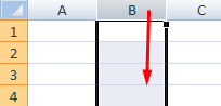
Для выделения строки – по названию строки (по цифре).
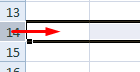
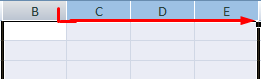
Чтобы выделить несколько столбцов или строк, щелкаем левой кнопкой мыши по названию, держим и протаскиваем.
Для выделения столбца с помощью горячих клавиш ставим курсор в любую ячейку нужного столбца – нажимаем Ctrl + пробел. Для выделения строки – Shift + пробел.
Как изменить границы ячеек
Если информация при заполнении таблицы не помещается нужно изменить границы ячеек:
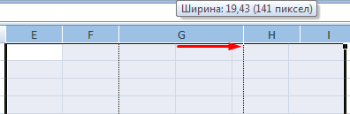
- Передвинуть вручную, зацепив границу ячейки левой кнопкой мыши.
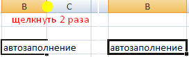
- Когда длинное слово записано в ячейку, щелкнуть 2 раза по границе столбца / строки. Программа автоматически расширит границы.
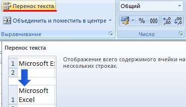
- Если нужно сохранить ширину столбца, но увеличить высоту строки, воспользуемся кнопкой «Перенос текста» на панели инструментов.
Для изменения ширины столбцов и высоты строк сразу в определенном диапазоне выделяем область, увеличиваем 1 столбец /строку (передвигаем вручную) – автоматически изменится размер всех выделенных столбцов и строк.
Примечание. Чтобы вернуть прежний размер, можно нажать кнопку «Отмена» или комбинацию горячих клавиш CTRL+Z. Но она срабатывает тогда, когда делаешь сразу. Позже – не поможет.
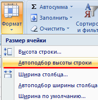
Чтобы вернуть строки в исходные границы, открываем меню инструмента: «Главная»-«Формат» и выбираем «Автоподбор высоты строки»
Для столбцов такой метод не актуален. Нажимаем «Формат» — «Ширина по умолчанию». Запоминаем эту цифру. Выделяем любую ячейку в столбце, границы которого необходимо «вернуть». Снова «Формат» — «Ширина столбца» — вводим заданный программой показатель (как правило это 8,43 — количество символов шрифта Calibri с размером в 11 пунктов). ОК.
Как вставить столбец или строку
Выделяем столбец /строку правее /ниже того места, где нужно вставить новый диапазон. То есть столбец появится слева от выделенной ячейки. А строка – выше.
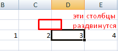
Нажимаем правой кнопкой мыши – выбираем в выпадающем меню «Вставить» (или жмем комбинацию горячих клавиш CTRL+SHIFT+»=»).
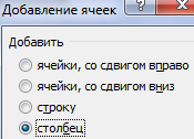
Отмечаем «столбец» и жмем ОК.
Совет. Для быстрой вставки столбца нужно выделить столбец в желаемом месте и нажать CTRL+SHIFT+»=».
Все эти навыки пригодятся при составлении таблицы в программе Excel. Нам придется расширять границы, добавлять строки /столбцы в процессе работы.
Пошаговое создание таблицы с формулами
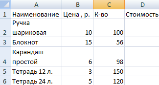
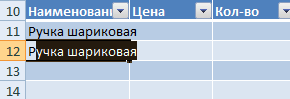
- Заполняем вручную шапку – названия столбцов. Вносим данные – заполняем строки. Сразу применяем на практике полученные знания – расширяем границы столбцов, «подбираем» высоту для строк.
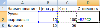
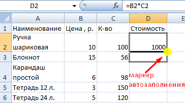
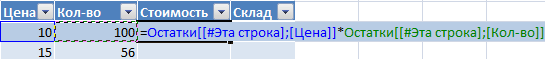
- Чтобы заполнить графу «Стоимость», ставим курсор в первую ячейку. Пишем «=». Таким образом, мы сигнализируем программе Excel: здесь будет формула. Выделяем ячейку В2 (с первой ценой). Вводим знак умножения (*). Выделяем ячейку С2 (с количеством). Жмем ВВОД.
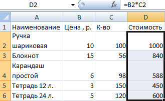
- Когда мы подведем курсор к ячейке с формулой, в правом нижнем углу сформируется крестик. Он указываем на маркер автозаполнения. Цепляем его левой кнопкой мыши и ведем до конца столбца. Формула скопируется во все ячейки.
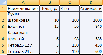
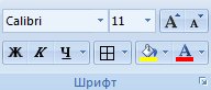
- Обозначим границы нашей таблицы. Выделяем диапазон с данными. Нажимаем кнопку: «Главная»-«Границы» (на главной странице в меню «Шрифт»). И выбираем «Все границы».
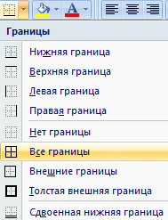
Теперь при печати границы столбцов и строк будут видны.
С помощью меню «Шрифт» можно форматировать данные таблицы Excel, как в программе Word.
Поменяйте, к примеру, размер шрифта, сделайте шапку «жирным». Можно установить текст по центру, назначить переносы и т.д.
Как создать таблицу в Excel: пошаговая инструкция
Простейший способ создания таблиц уже известен. Но в Excel есть более удобный вариант (в плане последующего форматирования, работы с данными).
Сделаем «умную» (динамическую) таблицу:
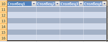
- Переходим на вкладку «Вставка» — инструмент «Таблица» (или нажмите комбинацию горячих клавиш CTRL+T).
- В открывшемся диалоговом окне указываем диапазон для данных. Отмечаем, что таблица с подзаголовками. Жмем ОК. Ничего страшного, если сразу не угадаете диапазон. «Умная таблица» подвижная, динамическая.

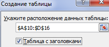
Примечание. Можно пойти по другому пути – сначала выделить диапазон ячеек, а потом нажать кнопку «Таблица».
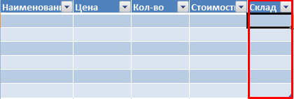
Теперь вносите необходимые данные в готовый каркас. Если потребуется дополнительный столбец, ставим курсор в предназначенную для названия ячейку. Вписываем наименование и нажимаем ВВОД. Диапазон автоматически расширится.
Если необходимо увеличить количество строк, зацепляем в нижнем правом углу за маркер автозаполнения и протягиваем вниз.
Как работать с таблицей в Excel
С выходом новых версий программы работа в Эксель с таблицами стала интересней и динамичней. Когда на листе сформирована умная таблица, становится доступным инструмент «Работа с таблицами» — «Конструктор».

Здесь мы можем дать имя таблице, изменить размер.
Доступны различные стили, возможность преобразовать таблицу в обычный диапазон или сводный отчет.
Возможности динамических электронных таблиц MS Excel огромны. Начнем с элементарных навыков ввода данных и автозаполнения:
- Выделяем ячейку, щелкнув по ней левой кнопкой мыши. Вводим текстовое /числовое значение. Жмем ВВОД. Если необходимо изменить значение, снова ставим курсор в эту же ячейку и вводим новые данные.
- При введении повторяющихся значений Excel будет распознавать их. Достаточно набрать на клавиатуре несколько символов и нажать Enter.
- Чтобы применить в умной таблице формулу для всего столбца, достаточно ввести ее в одну первую ячейку этого столбца. Программа скопирует в остальные ячейки автоматически.
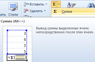
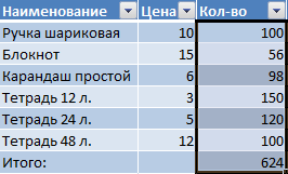
- Для подсчета итогов выделяем столбец со значениями плюс пустая ячейка для будущего итога и нажимаем кнопку «Сумма» (группа инструментов «Редактирование» на закладке «Главная» или нажмите комбинацию горячих клавиш ALT+»=»).
Если нажать на стрелочку справа каждого подзаголовка шапки, то мы получим доступ к дополнительным инструментам для работы с данными таблицы.
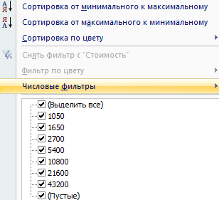
Иногда пользователю приходится работать с огромными таблицами. Чтобы посмотреть итоги, нужно пролистать не одну тысячу строк. Удалить строки – не вариант (данные впоследствии понадобятся). Но можно скрыть. Для этой цели воспользуйтесь числовыми фильтрами (картинка выше). Убираете галочки напротив тех значений, которые должны быть спрятаны.
A spreadsheet is a computer application that is designed to add, display, analyze, organize, and manipulate data arranged in rows and columns. It is the most popular application for accounting, analytics, data presentation, etc. Or in other words, spreadsheets are scalable grid-based files that are used to organize data and perform calculations. People all across the world use spreadsheets to create tables for personal and business usage. You can also use the tool’s features and formulas to help you make sense of your data. You could, for example, track data in a spreadsheet and see sums, differences, multiplication, division, and fill dates automatically, among other things. Microsoft Excel, Google sheets, Apache open office, LibreOffice, etc are some spreadsheet software. Among all these software, Microsoft Excel is the most commonly used spreadsheet tool and it is available for Windows, macOS, Android, etc.
A collection of spreadsheets is known as a workbook. Every Excel file is called a workbook. Every time when you start a new project in Excel, you’ll need to create a new workbook. There are several methods for getting started with an Excel workbook. To create a new worksheet or access an existing one, you can either start from scratch or utilize a pre-designed template.
A single Excel worksheet is a tabular spreadsheet that consists of a matrix of rectangular cells grouped in rows and columns. It has a total of 1,048,576 rows and 16,384 columns, resulting in 17,179,869,184 cells on a single page of a Microsoft Excel spreadsheet where you may write, modify, and manage your data.
In the same way as a file or a book is made up of one or more worksheets that contain various types of related data, an Excel workbook is made up of one or more worksheets. You can also create and save an endless number of worksheets. The major purpose is to collect all relevant data in one place, but in many categories (worksheet).
Feature of spreadsheet
As we know that there are so many spreadsheet applications available in the market. So these applications provide the following basic features:
1. Rows and columns: Rows and columns are two distinct features in a spreadsheet that come together to make a cell, a range, or a table. In general, columns are the vertical portion of an excel worksheet, and there can be 256 of them in a worksheet, whereas rows are the horizontal portion, and there can be 1048576 of them.
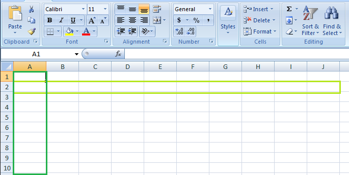
The color light green is used to highlight Row 3 while the color green is used to highlight Column B. Each column has 1048576 rows and each row has 256 columns.
2. Formulas: In spreadsheets, formulas process data automatically. It takes data from the specified area of the spreadsheet as input then processes that data, and then displays the output into the new area of the spreadsheet according to where the formula is written. In Excel, we can use formulas simply by typing “=Formula Name(Arguments)” to use predefined Excel formulas. When you write the first few characters of any formula, Excel displays a drop-down menu of formulas that match that character sequence. Some of the commonly used formulas are:
- =SUM(Arg1: Arg2): It is used to find the sum of all the numeric data specified in the given range of numbers.
- =COUNT(Arg1: Arg2): It is used to count all the number of cells(it will count only number) specified in the given range of numbers.
- =MAX(Arg1: Arg2): It is used to find the maximum number from the given range of numbers.
- =MIN(Arg1: Arg2): It is used to find the minimum number from the given range of numbers.
- =TODAY(): It is used to find today’s date.
- =SQRT(Arg1): It is used to find the square root of the specified cell.
For example, you can use the formula to find the average of the integers in column C from row 2 to row 7:
= AVERAGE(D2:D7)
The range of values on which you want to average is defined by D2:D6. The formula is located near the name field on the formula tab.
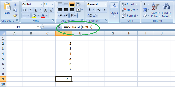
We wrote =AVERAGE(D2:D6) in cell D9, therefore the average becomes (2 + 3 + 4 + 5 + 6 + 7)/6 = 27/6 = 4.5. So you can quickly create a workbook, work on it, browse through it, and save it in this manner.
3. Function: In spreadsheets, the function uses a specified formula on the input and generates output. Or in other words, functions are created to perform complicated math problems in spreadsheets without using actual formulas. For example, you want to find the total of the numeric data present in the column then use the SUM function instead of adding all the values present in the column.
4. Text Manipulation: The spreadsheet provides various types of commands to manipulate the data present in it.
5. Pivot Tables: It is the most commonly used feature of the spreadsheet. Using this table users can organize, group, total, or sort data using the toolbar. Or in other words, pivot tables are used to summarize lots of data. It converts tons of data into a few rows and columns.
Use of Spreadsheets
The use of Spreadsheets is endless. It is generally used with anything that contains numbers. Some of the common use of spreadsheets are:
- Finance: Spreadsheets are used for financial data like it is used for checking account information, taxes, transaction, billing, budgets, etc.
- Forms: Spreadsheet is used to create form templates to manage performance review, timesheets, surveys, etc.
- School and colleges: Spreadsheets are most commonly used in schools and colleges to manage student’s data like their attendance, grades, etc.
- Lists: Spreadsheets are also used to create lists like grocery lists, to-do lists, contact detail, etc.
- Hotels: Spreadsheets are also used in hotels to manage the data of their customers like their personal information, room numbers, check-in date, check-out date, etc.
Components of Spreadsheets
The basic components of spreadsheets are:
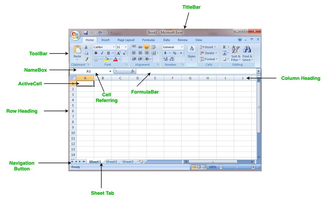
1. TitleBar: The title bar displays the name of the spreadsheet and application.
2. Toolbar: It displays all the options or commands available in Excel for use.
3. NameBox: It displays the address of the current or active cell.
4. Formula Bar: It is used to display the data entered by us in the active cell. Also, this bar is used to apply formulas to the data of the spreadsheet.
5. Column Headings: Every excel spreadsheet contains 256 columns and each column present in the spreadsheet is named by letters or a combination of letters.
6. Row Headings: Every excel spreadsheet contains 65,536 rows and each row present in the spreadsheet is named by a number.
7. Cell: In a spreadsheet, everything like a numeric value, functions, expressions, etc., is recorded in the cell. Or we can say that an intersection of rows and columns is known as a cell. Every cell has its own name or address according to its column and rows and when the cursor is present on the first cell then that cell is known as an active cell.
8. Cell referring: A cell reference, also known as a cell address, is a way for describing a cell on a worksheet that combines a column letter and a row number. We can refer to any cell on the worksheet using cell references (in excel formulae). As shown in the above image the cell in column A and row 1 is referred to as A1. Such notations can be used in any formula or to duplicate the value of one cell to another (by using = A1).
9. Navigation buttons: A spreadsheet contains first, previous, next, and last navigation buttons. These buttons are used to move from one worksheet to another workbook.
10. Sheet tabs: As we know that a workbook is a collection of worksheets. So this tab contains all the worksheets present in the workbook, by default it contains three worksheets but you can add more according to your requirement.
Create a new Spreadsheet or Workbook
To create a new spreadsheet follow the following steps:
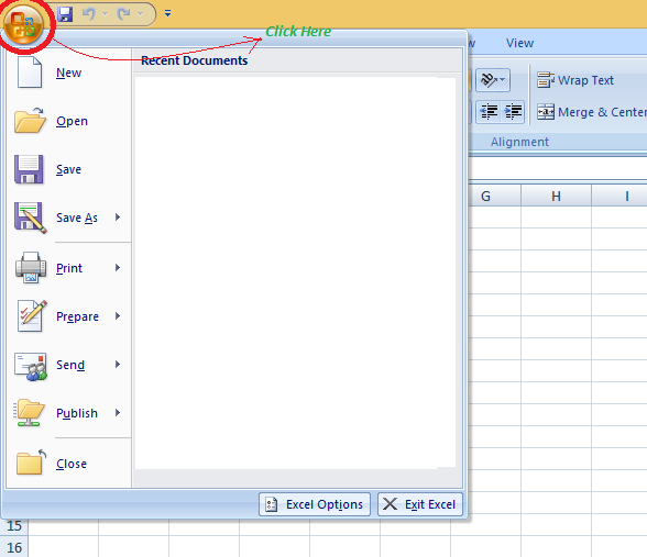
Step 1: Click on the top-left, Microsoft office button and a drop-down menu appear.
Step 2: Now select New from the menu.
Step 3: After selecting the New option a New Workbook dialogue box will appear and then in Create tab, click on the blank Document.
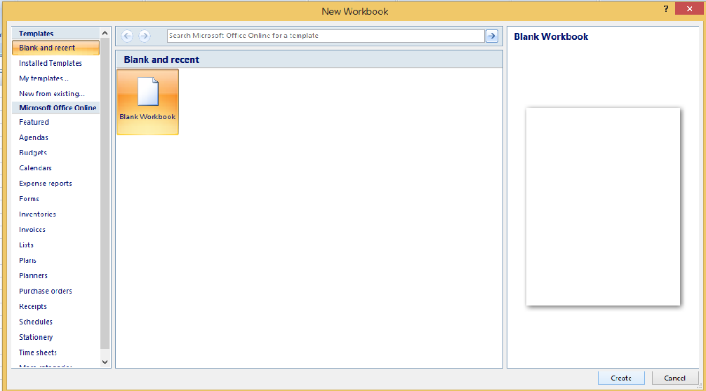
A new blank worksheet is created and is shown on your screen.
Note: When you open MS Excel on your computer, it creates a new Workbook for you.
Saving The Workbook
In Excel we can save a workbook using the following steps:
Step 1: Click on the top-left, Microsoft office button and we get a drop-down menu:
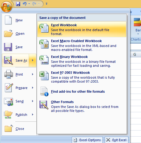
Step 2: Now Save or Save As are the options to save the workbook, so choose one.
- Save As: To name the spreadsheet and then save it to a specific location. Select Save As if you wish to save the file for the first time, or if you want to save it with a new name.
- Save: To save your work, select Save/ click ctrl + S if the file has already been named.
So this is how you can save a workbook in Excel.
Inserting text in Spreadsheet
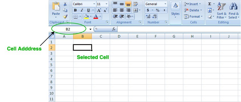
Excel consists of many rows and columns, each rectangular box in a row or column is referred to as a Cell. So, the combination of a column letter and a row number can be used to find a cell address on a worksheet or spreadsheet. We can refer to any cell in the worksheet using these addresses (in excel formulas). The name box on the top left(below the Home tab) displays the cell’s address whenever you click the cell.
To insert the data into the cell follow the following steps:
Step 1: Go to a cell and click on it
Step 2: By typing something on the keyboard, you can insert your data (In that selected cell).
Whatever text you type displays in the formula bar as well (for that cell).
Edit/ Delete Cell Contents in the Spreadsheet
To delete cell content follow the following steps:
Step 1: To alter or delete the text in a cell, first select it.
Step 2: Press the Backspace key on your keyboard to delete and correct text. Alternatively, hit the Delete key to delete the whole contents of a cell. You can also edit and delete text using the formula bar. Simply select the cell and move the pointer to the formula bar.
![]()
Download Article
![]()
Download Article
Do you need to create a spreadsheet in Microsoft Excel but have no idea where to begin? You’ve come to the right place! While Excel can be intimidating at first, creating a basic spreadsheet is as simple as entering data into numbered rows and lettered columns. Whether you need to make a spreadsheet for school, work, or just to keep track of your expenses, this wikiHow article will teach you everything you know about editing your first spreadsheet in Microsoft Excel.
-

1
Open Microsoft Excel. You’ll find it in the Start menu (Windows) or in the Applications folder (macOS). The app will open to a screen that allows you to create or select a document.
- If you don’t have a paid version of Microsoft Office, you can use the free online version at https://www.office.com to create a basic spreadsheet. You’ll just need to sign in with your Microsoft account and click Excel in the row of icons.
-
2
Click Blank workbook to create a new workbook. A workbook is the name of the document that contains your spreadsheet(s). This creates a blank spreadsheet called Sheet1, which you’ll see on the tab at the bottom of the sheet.
- When you make more complex spreadsheets, you can add another sheet by clicking + next to the first sheet. Use the bottom tabs to switch between spreadsheets.
Advertisement
-
3
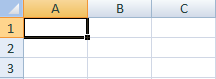
Familiarize yourself with the spreadsheet’s layout. The first thing you’ll notice is that the spreadsheet contains hundreds of rectangular cells organized into vertical columns and horizontal rows. Some important things to note about this layout:
- All rows are labeled with numbers along the side of the spreadsheet, while the columns are labeled with letters along the top.
- Each cell has an address consisting of the column letter followed by the row number. For example, the address of the cell in the first column (A), first row (1) is A1. The address of the cell in column B row 3 is B3.
-
4
Enter some data. Click any cell one time and start typing immediately. When you’re finished with that cell, press the Tab ↹ key to move to the next cell in the row, or the ↵ Enter key to the next cell in the column.
- Notice that as you type into the cell, the content also appears in the bar that runs across the top of the spreadsheet. This bar is called the Formula Bar and is useful for when entering long strings of data and/or formulas.[1]
- To edit a cell that already has data, double-click it to bring back the cursor. Alternatively, you can click the cell once and make your changes in the formula bar.
- To delete the data from one cell, click the cell once, and then press Del. This returns the cell to a blank one without messing up the data in other rows or columns. To delete multiple cell values at once, press Ctrl (PC) or ⌘ Cmd (Mac) as you click each cell you want to delete, and then press Del.
- To add a new blank column between existing columns, right-click the letter above the column after where you’d like the new one to appear, and then click Insert on the context menu.
- To add a new blank row between existing rows, right-click the row number for the row after the desired location, and then click Insert on the menu.
- Notice that as you type into the cell, the content also appears in the bar that runs across the top of the spreadsheet. This bar is called the Formula Bar and is useful for when entering long strings of data and/or formulas.[1]
-
5
Check out the functions available for advanced uses. One of the most useful features of Excel is its ability to look up data and perform calculations based on mathematical formulas. Each formula you create contains an Excel function, which is the «action» you’re performing. Formulas always begin with an equal (=) sign followed by the function name (e.g., =SUM, =LOOKUP, =SIN). After that, the parameters should be entered between a set of parentheses (). Follow these steps to get an idea of the type of functions you can use in Excel:
- Click the Formulas tab at the top of the screen. You’ll notice several icons in the toolbar at the top of the application in the panel labeled «Function Library.» Once you know how the different functions work, you can easily browse the library using those icons.
- Click the Insert Function icon, which also displays an fx. It should be the first icon on the bar. This opens the Insert Function panel, which allows you to search for what you want to do or browse by category.
- Select a category from the «Or select a category» menu. The default category is «Most Recently Used.» For example, to see the math functions, you might select Math & Trig.
- Click any function in the «Select a function» panel to view its syntax, as well as a description of what the function does. For more info on a function, click the Help on this function.
- Click Cancel when you’re done browsing.
- To learn more about entering formulas, see How to Type Formulas in Microsoft Excel.
-
6
Save your file when you’re finished editing. To save the file, click the File menu at the top-left corner, and then select Save As. Depending on your version of Excel, you’ll usually have the option to save the file to your computer or OneDrive.
- Now that you’ve gotten the hang of the basics, check out the «Creating a Home Inventory from Scratch» method to see this information put into practice.


Advertisement
-
1
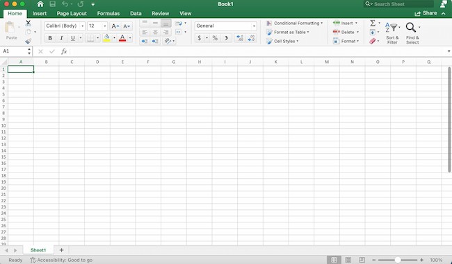
Open Microsoft Excel. You’ll find it in the Start menu (Windows) or in the Applications folder (macOS). The app will open to a screen that allows you to create or open a workbook.
-
2
Name your columns. Let’s say we’re making a list of items in our home. In addition to listing what the item is, we might want to record which room it’s in and its make/model. We’ll reserve row 1 for column headers so our data is clearly labeled. [2]
.- Click cell A1 and type Item. We’ll list each item in this column.
- Click cell B1 and type Location. This is where we’ll enter which room the item is in.
- Click cell C1 and type Make/Model. We’ll list the item’s model and manufacturer in this column.
-
3
Enter your items on each row. Now that our columns are labeled, entering our data into the rows should be simple. Each item should get its own row, and each bit of information should get its own cell.
- For example, if you’re listening the Apple HD monitor in your office, you may type HD monitor into A2 (in the Item column), Office into B2 (in the Location column), and Apple Cinema 30-inch M9179LL into B3 (the Make/Model column).
- List additional items on the rows below. If you need to delete a cell, just click it once and press Del.
- To remove an entire row or column, right-click the letter or number and select Delete.
- You’ve probably noticed that if you type too much text in a cell it’ll overlap into the next column. You can fix this by resizing the columns to fit the text. Position the cursor on the line between the column letters (above row 1) so the cursor turns into two arrows, and then double-click that line.
-
4
Turn the column headers into drop-down menus. Let’s say you’ve listed hundreds of items throughout your home but only want to view those stored in your office. Click the 1 at the beginning of row 1 to select the whole row, and then do the following:
- Click the Data tab at the top of Excel.
- Click Filter (the funnel icon) in the toolbar. Small arrows now appear on each column header.
- Click the Location drop-down menu (in B1) to open the filter menu.
- Since we just want to see items in the office, check the box next to «Office» and remove the other checkmarks.
- Click OK. Now you’ll only see items the selected room. You can do this with any column and any data type.
- To restore all items, click the menu again and check «Select All» and then OK to restore all items.
-
5
Click the Page Layout tab to customize the spreadsheet. Now that you’ve entered your data, you may want to customize the colors, fonts, and lines. Here are some ideas for doing so:
- Select the cells you want to format. You can select an entire row by clicking its number, or an whole column by clicking its letter. Hold Ctrl (PC) or Cmd (Mac) to select more than one column or row at a time.
- Click Colors in the «Themes» area of the toolbar to view and select color theme.
- Click the Fonts menu to browse for and select a font.
-
6
Save your document. When you’ve reached a good stopping point, you can save the spreadsheet by clicking the File menu at the top-left corner and selecting Save As.


Advertisement
-
1
Open Microsoft Excel. You’ll find it in the Start menu (Windows) or in the Applications folder (macOS). The app will open to a screen that allows you to create or open a workbook.
- This method covers using a built-in Excel template to create a list of your expenses. There are hundreds of templates available for different types of spreadsheets. To see a list of all official templates, visit https://templates.office.com/en-us/templates-for-excel.
-
2
Search for the «Simple Monthly Budget» template. This is a free official Microsoft template that makes it easy to calculate your budget for the month. You can find it by typing Simple Monthly Budget into the search bar at the top and pressing ↵ Enter in most versions.
-
3
Select the Simple Monthly Budget template and click Create. This creates a new spreadsheet from a pre-formatted template.
- You may have to click Download instead.
-
4
Click the Monthly Income tab to enter your income(s). You’ll notice there are three tabs (Summary, Monthly Income, and Monthly Expenses) at the bottom of the workbook. You’ll be clicking the second tab. Let’s say you get income from two companies called wikiHow and Acme:
- Double-click the Income 1 cell to bring up the cursor. Erase the content of the cell and type wikiHow.
- Double-click the Income 2 cell, erase the contents, and type Acme.
- Enter your monthly income from wikiHow into the first cell under the «Amount» header (the one that says «2500» by default). Do the same with your monthly income from «Acme» in the cell just below.
- If you don’t have any other income, you can click the other cells (for «Other» and «$250») and press Del to clear them.
- You can also add more income sources and amounts in the rows below those that already exist.
-
5
Click the Monthly Expenses tab to enter your expenses. It’s the third tab at the bottom of the workbook. Those there are expenses and amounts already filled in, you can double-click any cell to change its value.
- For example, let’s say your rent is $795/month. Double-click the pre-filled amount of «$800,» erase it, and then type 795.
- Let’s say you don’t have any student loan payments to make. You can just click the amount next to «Student Loans» in the «Amount» column ($50) and press Del on your keyboard to clear it. Do the same for all other expenses.
- You can delete an entire row by right-clicking the row number and selecting Delete.
- To insert a new row, right-click the row number below where you want it to appear, and then select Insert.
- Make sure there are no extra amounts that you don’t actually have to pay in the «Amounts» column, as they’ll be automatically factored into your budget.
-
6
Click the Summary tab to visualize your budget. Once you’ve entered your data, the chart on this tab will automatically update to reflect your income vs. your expenses.
- If the info doesn’t calculate automatically, press F9 on the keyboard.
- Any changes you make to the Monthly Income and Monthly Expenses tabs will affect what you see in your Summary.
-
7
Save your document. When you’ve reached a good stopping point, you can save the spreadsheet by clicking the File menu at the top-left corner and selecting Save As.


Advertisement
Add New Question
-
Question
How do I name a spreadsheet?

When you click «Save As,» at the bottom of the page there should be a file name box. Whatever you type into that box will be your spreadsheet’s name.
-
Question
Can I rename the columns, instead of A, B, C, etc.?
You cannot change those labels. Typically, the name of the column is simply written in the first row.
-
Question
How do I make more space to type in the boxes?
As you’re typing, select the cell where you want the text to be and select «Wrap Text» at the top of the page. This will contain all of the text to the same cell, which will grow as you type.
See more answers
Ask a Question
200 characters left
Include your email address to get a message when this question is answered.
Submit
Advertisement
Thanks for submitting a tip for review!
About This Article
Article SummaryX
1. Open Excel.
2. Click New Blank Workbook.
3. Enter column headers into row 1.
4. Enter data on individual rows.
5. Click the Page Layout tab to format the data.
6. Click File > Save As to save the document.
Did this summary help you?
Thanks to all authors for creating a page that has been read 2,886,243 times.
Is this article up to date?
Microsoft Excel know-how is so expected that it hardly warrants a line on a resume anymore. But how well do you really know how to use it?
Marketing is more data-driven than ever before. At any time you could be tracking growth rates, content analysis, or marketing ROI. You may know how to plug in numbers and add up cells in a column in Excel, but that’s not going to get you far when it comes to metrics reporting.
![Download 10 Excel Templates for Marketers [Free Kit]](https://no-cache.hubspot.com/cta/default/53/9ff7a4fe-5293-496c-acca-566bc6e73f42.png)
Do you want to understand what pivot tables are? Are you ready for your first VLOOKUP? Aspiring Excel wizard, read on or jump to the section that interests you most:
What is Microsoft Excel?
Microsoft Excel is a popular spreadsheet software program for business. It’s used for data entry and management, charts and graphs, and project management. You can format, organize, visualize, and calculate data with this tool.
How to Download Microsoft Excel
It’s easy to download Microsoft Excel. First, check to make sure that your PC or Mac meets Microsoft’s system requirements. Next, sign in and install Microsoft 365.
After you sign in, follow the steps for your account and computer system to download and launch the program.
For example, say you’re working on a Mac desktop. You’ll click on Launchpad or look in your applications folder. Then, click on the Excel icon to open the application.
Microsoft Excel Spreadsheet Basics
Sometimes, Excel seems too good to be true. Need to combine data in multiple cells? Excel can do it. Need to copy formatting across an array of cells? Excel can do that, too.
Let’s start this Excel guide with the basics. Once you have these functions down, you’ll be ready to tackle more pro Excel tips and advanced lessons.
Inserting Rows or Columns
As you work with data, you might find yourself needing to add more rows and columns. Doing this one at a time would be super tedious. Luckily, there’s an easier way.
To add multiple rows or columns in a spreadsheet, highlight the number of pre-existing rows or columns that you want to add. Then, right-click and select «Insert.»
In this example, I add three rows to the top of my spreadsheet.
Autofill
Autofill lets you quickly fill adjacent cells with several types of data, including values, series, and formulas.
There are many ways to deploy this feature, but the fill handle is among the easiest.
First, choose the cells you want to be the source. Next, find the fill handle in the lower-right corner of the cell. Then either drag the fill handle to cover the cells you want to fill or just double-click.
Filters
When you’re looking at large data sets, you usually don’t need to look at every row at the same time. Sometimes, you only want to look at data that fit into certain criteria. That’s where filters come in.
Filters allow you to pare down data to only see certain rows at one time. In Excel, you can add a filter to each column in your data. From there, you can choose which cells you want to view.
To add a filter, click the Data tab and select «Filter.» Next, click the arrow next to the column headers. This lets you choose whether you want to organize your data in ascending or descending order, as well as which rows you want to show.
Let’s take a look at the Harry Potter example below. Say you only want to see the students in Gryffindor. By selecting the Gryffindor filter, the other rows disappear.
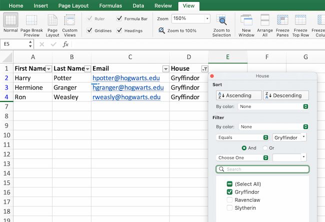
Pro tip: Start with a filtered view in your original spreadsheet. Then, copy and paste the values to another spreadsheet before you start analyzing.
Sort
Sometimes you’ll have a disorganized list of data. This is typical when you’re exporting lists, like marketing contacts or blog posts. Excel’s sort feature can help you alphabetize any list.
Click on the data in the column you want to sort. Then click on the «Data» tab in your toolbar and look for the «Sort» option on the left.
- If the «A» is on top of the «Z,» you can just click on that button once. Choosing A-Z means the list will sort in alphabetical order.
- If the «Z» is on top of the «A,» click the button twice. Z-A selection means the list will sort in reverse alphabetical order.
Remove Duplicates
Large datasets tend to have duplicate content. For example, you may have a list of different company contacts, but you only want to see the number of companies you have. In situations like this, removing duplicates comes in handy.
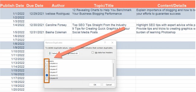
To remove duplicates, highlight the row or column where you noticed duplicate data. Then, go to the Data tab, and select «Remove Duplicates» (under Tools). A pop-up will appear so that you can confirm which data you want to keep. Select «Remove Duplicates,» and you’re good to go.
If you want to see an example, this post offers step-by-step instructions for removing duplicates.
You can also use this feature to remove an entire row based on a duplicate column value. So, say you have three rows of information and you only need to see one, you can select the whole dataset and then remove duplicates. The resulting list will have only unique data without any duplicates.
Paste Special
It’s often helpful to change the items in a row of data into a column (or vice versa). It would take a lot of time to copy and paste each individual header.
Not to mention, you may easily fall into one of the biggest, most unfortunate Excel traps — human error. Read here to check out some of the most common Microsoft Excel errors.
Instead of making one of these errors, let Excel do the work for you. Take a look at this example:
To use this function, highlight the column or row you want to transpose. Then, right-click and select «Copy.»
Next, select the cells where you want the first row or column to begin. Right-click on the cell, and then select «Paste Special.»
When the module appears, choose the option to transpose.
Paste Special is a super useful function. In the module, you can also choose between copying formulas, values, formats, or even column widths. This is especially helpful when it comes to copying the results of your pivot table into a chart.
Text to Columns
What if you want to split out information that’s in one cell into two different cells? For example, maybe you want to pull out someone’s company name through their email address. Or you want to separate someone’s full name into a first and last name for your email marketing templates.
Thanks to Microsoft Excel, both are possible. First, highlight the column where you want to split up. Next, go to the Data tab and select «Text to Columns.» A module will appear with more information. First, you need to select either «Delimited» or «Fixed Width.»
- Delimited means you want to break up the column based on characters such as commas, spaces, or tabs.
- Fixed Width means you want to select the exact location in all the columns where you want the split to occur.
Select «Delimited» to separate the full name into first name and last name.
Then, it’s time to choose the delimiters. This could be a tab, semicolon, comma, space, or something else. (For example, «something else» could be the «@» sign used in an email address.) Let’s choose the space for this example. Excel will then show you a preview of what your new columns will look like.
When you’re happy with the preview, press «Next.» This page will allow you to select Advanced Formats if you choose to. When you’re done, click «Finish.»
Format Painter
Excel has a lot of features to make crunching numbers and analyzing your data quick and easy. But if you ever spent some time formatting a spreadsheet, you know it can get a bit tedious.
Don’t waste time repeating the same formatting commands over and over again. Use the format painter to copy formatting from one area of the worksheet to another.
To do this, choose the cell you’d like to replicate. Then, select the format painter option (paintbrush icon) from the top toolbar. When you release the mouse, your cell should show the new format.
Keyboard Shortcuts
Creating reports in Excel is time-consuming enough. How can we spend less time navigating, formatting, and selecting items in our spreadsheet? Glad you asked. There are a ton of Excel shortcuts out there, including some of our favorites listed below.
Create a New Workbook
PC: Ctrl-N | Mac: Command-N
Select Entire Row
PC: Shift-Space | Mac: Shift-Space
Select Entire Column
PC: Ctrl-Space | Mac: Control-Space
Select Rest of Column
PC: Ctrl-Shift-Down/Up | Mac: Command-Shift-Down/Up
Select Rest of Row
PC: Ctrl-Shift-Right/Left | Mac: Command-Shift-Right/Left
Add Hyperlink
PC: Ctrl-K | Mac: Command-K
Open Format Cells Window
PC: Ctrl-1 | Mac: Command-1
Autosum Selected Cells
PC: Alt-= | Mac: Command-Shift-T
Excel Formulas
At this point, you’re getting used to Excel’s interface and flying through quick commands on your spreadsheets.
Now, let’s dig into the core use case for the software: Excel formulas. Excel can help you do simple arithmetic like adding, subtracting, multiplying, or dividing any data.
- To add, use the + sign.
- To subtract, use the — sign.
- To multiply, use the * sign.
- To divide, use the / sign.
- To use exponents, use the ^ sign.
Remember, all formulas in Excel must begin with an equal sign (=). Use parentheses to make sure certain calculations happen first. For example, consider how =10+10*10 is different from =(10+10)*10.
Besides manually typing in simple calculations, you can also refer to Excel’s built-in formulas. Some of the most common include:
- Average: =AVERAGE(cell range)
- Sum: =SUM(cell range)
- Count: =COUNT(cell range)
Also note that series’ of specific cells are separated by a comma (,), while cell ranges are notated with a colon (:). For example, you could use any of these formulas:
- =SUM(4,4)
- =SUM(A4,B4)
- =SUM(A4:B4)
Conditional Formatting
Conditional formatting lets you change a cell’s color based on the information within the cell. For example, say you want to flag a category in your spreadsheet.
To get started, highlight the group of cells you want to use conditional formatting on. Then, choose «Conditional Formatting» from the Home menu. Next, select a logic option from the dropdown. A window will pop up that prompts you to provide more information about your formatting rule. Select «OK» when you’re done, and you should see your results automatically appear.
Note: You can also create your own logic if you want something beyond the dropdown choices.
Dollar Signs
Have you ever seen a dollar sign in an Excel formula? When this symbol is in a formula, it isn’t representing an American dollar. Instead, it makes sure that the exact column and row stay the same even if you copy the same formula in adjacent rows.
You see, a cell reference — when you refer to cell A5 from cell C5, for example — is relative by default.
This means you’re actually referring to a cell that’s five columns to the left (C minus A) and in the same row (5). This is called a relative formula.
When you copy a relative formula from one cell to another, it’ll adjust the values in the formula based on where it’s moved. But sometimes, you want those values to stay the same no matter whether they’re moved around or not. You can do that by making the formula in the cell into what’s called an absolute formula.
To change the relative formula (=A5+C5) into an absolute formula, precede the row and column values with dollar signs, like this: (=$A$5+$C$5).
Combine Cells Using «&»
Databases tend to split out data to make it as exact as possible. For example, instead of having data that shows a person’s full name, a database might have the data as a first name and then a last name in separate columns.
In Excel, you can combine cells with different data into one cell by using the «&» sign in your function. The example below uses this formula: =A2&» «&B2.
Let’s go through the formula together using an example. So, let’s combine first names and last names into full names in a single column.
To do this, put your cursor in the blank cell where you want the full name to appear. Next, highlight one cell that contains a first name, type in an «&» sign, and then highlight a cell with the corresponding last name.
But you’re not finished. If all you type in is =A2&B2, then there will not be a space between the person’s first name and last name. To add that necessary space, use the function =A2&» «&B2. The quotation marks around the space tell Excel to put a space between the first and last name.
To make this true for multiple rows, drag the corner of that first cell downward as shown in the example.
Pivot Tables
Pivot tables reorganize data in a spreadsheet. A pivot table won’t change the data that you have, but it can sum up values and compare information in a way that’s easy to understand.
For example, let’s look at how many people are in each house at Hogwarts.
To create the Pivot Table, go to Insert > Pivot Table. Excel will automatically populate your pivot table, but you can always change the order of the data. Then, you have four options to choose from.
Report Filter
This allows you to only look at certain rows in your dataset.
For example, to create a filter by house, choose only students in Gryffindor.
Column and Row Labels
These could be any headers or rows in the dataset.
Note: Both Row and Column labels can contain data from your columns. For example, you can drag First Name to either the Row or Column label depending on how you want to see the data.
Value
This section allows you to convert data into a number. Instead of just pulling in any numeric value, you can sum, count, average, max, min, count numbers, or do a few other manipulations with your data. By default, when you drag a field to Value, it always does a count.
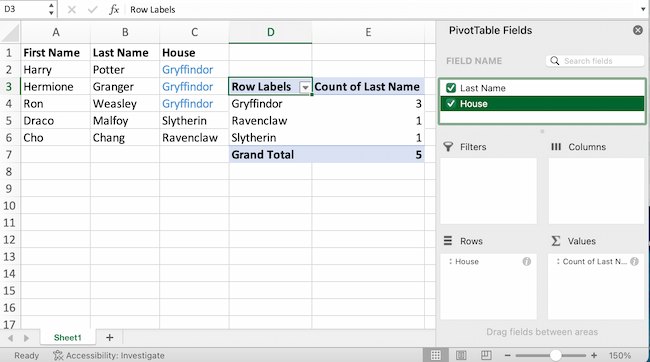
The example above counts the number of students in each house. To recreate this pivot table, go to the pivot table and drag the House column to both the row Labels and the values. This will sum up the number of students associated with each house.
IF Functions
At its most basic level, Excel’s IF function lets you see if a condition you set is true or false for a given value.
If the condition is true, you get one result. If the condition is false, you get another result.
This popular tool is useful for comparisons and finding errors. But if you’re new to Excel you may need a little more information to get the most out of this feature.
Let’s take a look at this function’s syntax:
- =IF(logical_test, value_if_true, [value_if_false])
- With values, this could be: =IF(A2>B2, «Over Budget», «OK»)
In this example, you want to find where you’re overspending. With this IF function, if your spending (what’s in A2) is greater than your budget (what’s in B2), that overspending will be easy to see. Then you can then filter the data so that you see only the line items where you’re going over budget.
The real power of the IF function comes when you string or «nest» multiple IF statements together. This allows you to set multiple conditions, get more specific results, and organize your data into more manageable chunks.
For example, ranges are one way to segment your data for better analysis. For example, you can categorize data into values that are less than 10, 11 to 50, or 51 to 100.
- =IF(B3<11,»10 or less»,IF(B3<51,»11 to 50″,IF(B3<100,»51 to 100″)))
Let’s talk about a few more IF functions.
COUNTIF Function
The power of IF functions goes beyond simple true and false statements. With the COUNTIF function, Excel can count the number of times a word or number appears in any range of cells.
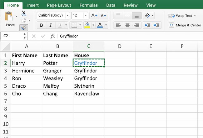
For example, let’s say you want to count the number of times the word «Gryffindor» appears in this data set.
Take a look at the syntax.
- The formula: =COUNTIF(range, criteria)
- The formula with variables from the example below: =COUNTIF(D:D,»Gryffindor»)
In this formula, there are several variables:
Range
The range that you want the formula to cover.
In this one-column example, «D:D» shows that the first and last columns are both D. If you want to look at columns C and D, use «C:D.»
Criteria
Whatever number or piece of text you want Excel to count.
Only use quotation marks if you want the result to be text instead of a number. In this example, «Gryffindor» is the only criteria.
To use this function, type the COUNTIF formula in any cell and press «Enter.» Using the example above, this action will show how many times the word «Gryffindor» appears in the dataset.
SUMIF Function
Ready to make the IF function a bit more complex? Let’s say you want to analyze the number of leads your blog has generated from one author, not the entire team.
With the SUMIFS function, you can add up cells that meet certain criteria. You can add as many different criteria to the formula as you like.
Here’s your formula:
- =SUMIFS(sum_range, criteria_range1, criteria1, [criteria_range2, criteria 2],etc.)
That’s a lot of criteria. Let’s take a look at each part:
Sum_range
The range of cells you’re going to add up.
Criteria_range1
The range that is being searched for your first value.
Criteria1
This is the specific value that determines which cells in Criteria_range1 to add together.
Note: Remember to use quotation marks if you’re searching for text.
In the example below, the SUMIF formula counts the total number of house points from Gryffindor.

If AND/OR
The OR and AND functions round out your IF function choices. These functions check multiple arguments. It returns either TRUE or FALSE depending on if at least one of the arguments is true (this is the OR function), or if all of them are true (this is the AND function).
Lost in a sea of «and’s» and «or’s»? Don’t check out yet. In practice, OR and AND functions will never be used on their own. They need to be nested inside of another IF function. Recall the syntax of a basic IF function:
- =IF(logical_test, value_if_true, [value_if_false])
- Now, let’s fit an OR function inside of the logical_test: =IF(OR(logical1, logical2), value_if_true, [value_if_false])
To put it plainly, this combined formula allows you to return a value if both conditions are true, as opposed to just one. With AND/OR functions, your formulas can be as simple or complex as you want them to be, as long as you understand the basics of the IF function.
VLOOKUP
Have you ever had two sets of data on two different spreadsheets that you want to combine into a single spreadsheet?
For example, say you have a list of names and email addresses in one spreadsheet and a list of email addresses and company names in a different spreadsheet. But you want the names, email addresses, and company names of those people to appear in one spreadsheet.
VLOOKUP is a great go-to formula for this.
Before you use the formula, be sure that you have at least one column that appears identically in both places.
Note: Scour your data sets to make sure the column of data you’re using to combine spreadsheets is exactly the same. This includes removing any extra spaces.
In the example below, Sheet One and Sheet Two are both lists with different information about the same people. The common thread between the two is their email addresses. Let’s combine both datasets so that all the house information from Sheet Two translates over to Sheet One.
Type in the formula: =VLOOKUP(C2,Sheet2!A:B,2,FALSE). This will bring all the house data into Sheet One.
Now that you’ve seen how VLOOKUP works, let’s review the formula.
- The formula: =VLOOKUP(lookup value, table array, column number, [range lookup])
- The formula with variables from the example: =VLOOKUP(C2,Sheet2!A:B,2,FALSE)
In this formula, there are several variables.
Lookup Value
A value that LOOKUP searches for in an array. So, your lookup value is the identical value you have in both spreadsheets.
In the example, the lookup value is the first email address on the list, or cell 2 (C2).
Table Array
Table arrays hold column-oriented or tabular data, like the columns on Sheet Two you’re going to pull your data from.
This table array includes the column of data identical to your lookup value in Sheet One and the column of data you’re trying to copy to Sheet Two.
In the example, «A» means Column A in Sheet Two. The «B» means Column B.
So, the table array is «Sheet2!A:B.»
Column Number
Excel refers to columns as letters and rows as numbers. So, the column number is the selected column for the new data you want to copy.
In the example, this would be the «House» column. «House» is column 2 in the table array.
Note: Your range can be more than two columns. For example, if there are three columns on Sheet Two — Email, Age, and House — and you also want to bring House onto Sheet One, you can still use a VLOOKUP. You just need to change the «2» to a «3» so it pulls back the value in the third column. The formula for this would be: =VLOOKUP(C2:Sheet2!A:C,3,false).]
Range Lookup
This term means that you’re looking for a value within a range of values. You can also use the term «FALSE» to pull only exact value matches.
Note: VLOOKUP will only pull back values to the right of the column containing your identical data on the second sheet. This is why some people prefer to use the INDEX and MATCH functions instead.
INDEX MATCH
Like VLOOKUP, the INDEX and MATCH functions pull data from another dataset into one central location. Here are the main differences:
VLOOKUP is a much simpler formula.
If you’re working with large datasets that need thousands of lookups, the INDEX MATCH function will decrease load time in Excel.
INDEX MATCH formulas work right-to-left.
VLOOKUP formulas only work as a left-to-right lookup. So, if you need to do a lookup that has a column to the right of the results column, you’d have to rearrange those columns to do a VLOOKUP. This can be tedious with large datasets and lead to errors.
Let’s look at an example. Let’s say Sheet One contains a list of names and their Hogwarts email addresses. Sheet Two contains a list of email addresses and each student’s Patronus.
The information that lives in both sheets is the email addresses column. But, the column numbers for email addresses are different on the two sheets. So, you’d use the INDEX MATCH formula instead of VLOOKUP to avoid column-switching errors.
The INDEX MATCH formula is the MATCH formula nested inside the INDEX formula.
- The formula: =INDEX(table array, MATCH formula)
- This becomes: =INDEX(table array, MATCH (lookup_value, lookup_array))
- The formula with variables from the example: =INDEX(Sheet2!A:A,(MATCH(Sheet1!C:C,Sheet2!C:C,0)))
Here are the variables:
Table Array
The range of columns on Sheet Two that contain the new data you want to bring over to Sheet One.
In the example, «A» means Column A, and has the «Patronus» information for each person.
Lookup Value
This Sheet One column has identical values in both spreadsheets.
In the example, this is the «email» column on Sheet One, which is Column C. So, Sheet1!C:C.
Lookup Array
Again, an array is a group of values in rows and columns that you want to search.
In this example, the lookup array is the column in Sheet Two that contains identical values in both spreadsheets. So, the «email» column on Sheet Two, Sheet2!C:C.
Once you have your variables set, type in the INDEX MATCH formula. Add it where you want the combined information to populate.
Data Visualization
Now that you’ve learned formulas and functions, let’s make your analysis visual. With a beautiful graph, your audience will be able to process and remember your data more easily.
Create a Basic Graph
First, decide what type of graph to use. Bar charts and pie charts help you compare categories. Pie charts compare part of a whole and are often best when one of the categories is way larger than the others. Bar charts highlight incremental differences between categories. Finally, line charts can help display trends over time.
This post can help you find the best chart or graph for your presentation.
Next, highlight the data you want to turn into a chart. Then choose «Charts» in the top navigation. You can also use Insert > Chart if you have an older version of Excel. Then you can adjust and resize your chart until it makes the statement you’re hoping for.
Microsoft Excel Can Help Your Business Grow
Excel is a useful tool for any small business. Whether you’re focused on marketing, HR, sales, or service, these Microsoft Excel tips can boost your performance.
Whether you want to improve efficiency or productivity, Excel can help. You can find new trends and organize your data into usable insights. It can make your data analysis easier to understand and your daily tasks easier.
All it takes is a little know-how and some time with the software. So start learning, and get ready to grow.
Editor’s note: This post was originally published in April 2018 and has been updated for comprehensiveness.
