
Содержание
- Convert numbers into words
- Create the SpellNumber function to convert numbers to words
- Use the SpellNumber function in individual cells
- Save your SpellNumber function workbook
- Бесшовная интеграция Microsoft Excel и Word с помощью Python
- Openpyxl
- Python-docx
- Автоматизация Microsoft Excel
- Извлечение диаграммы
- Автоматизация Microsoft Word
- Результаты
- Исходный код
- How to Insert Excel Data Into Word (Tables, Files, Spreadsheets)
- Free video on inserting Excel data in a Word document
- What is an Excel Worksheet object?
- Embedding Excel objects in Word
- Linking Excel objects in Word
- Insert an Excel worksheet in a Word document
Convert numbers into words
Excel doesn’t have a default function that displays numbers as English words in a worksheet, but you can add this capability by pasting the following SpellNumber function code into a VBA (Visual Basic for Applications) module. This function lets you convert dollar and cent amounts to words with a formula, so 22.50 would read as Twenty-Two Dollars and Fifty Cents. This can be very useful if you’re using Excel as a template to print checks.
If you want to convert numeric values to text format without displaying them as words, use the TEXT function instead.
Note: Microsoft provides programming examples for illustration only, without warranty either expressed or implied. This includes, but is not limited to, the implied warranties of merchantability or fitness for a particular purpose. This article assumes that you are familiar with the VBA programming language, and with the tools that are used to create and to debug procedures. Microsoft support engineers can help explain the functionality of a particular procedure. However, they will not modify these examples to provide added functionality, or construct procedures to meet your specific requirements.
Create the SpellNumber function to convert numbers to words
Use the keyboard shortcut, Alt + F11 to open the Visual Basic Editor (VBE).
Note: You can also access the Visual Basic Editor by showing the Developer tab in your ribbon.
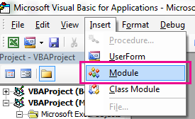
Click the Insert tab, and click Module.
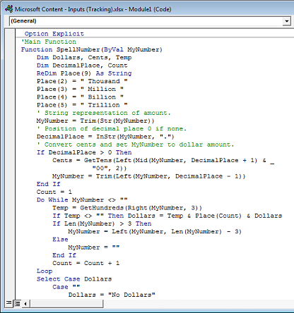
Copy the following lines of code.
Note: Known as a User Defined Function (UDF), this code automates the task of converting numbers to text throughout your worksheet.
Paste the lines of code into the Module1 (Code) box.
Press Alt + Q to return to Excel. The SpellNumber function is now ready to use.
Note: This function works only for the current workbook. To use this function in another workbook, you must repeat the steps to copy and paste the code in that workbook.
Use the SpellNumber function in individual cells
Type the formula =SpellNumber( A1) into the cell where you want to display a written number, where A1 is the cell containing the number you want to convert. You can also manually type the value like =SpellNumber(22.50).
Press Enter to confirm the formula.
Save your SpellNumber function workbook
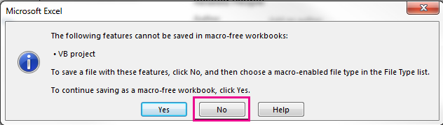
Excel cannot save a workbook with macro functions in the standard macro-free workbook format (.xlsx). If you click File > Save. A VB project dialog box opens. Click No.
You can save your file as an Excel Macro-Enabled Workbook (.xlsm) to keep your file in its current format.
Click File > Save As.
Click the Save as type drop-down menu, and select Excel Macro-Enabled Workbook.
Источник
Бесшовная интеграция Microsoft Excel и Word с помощью Python

Хотя в среднем для каждодневных задач автоматизация не требуется, бывают случаи, когда она может быть необходима. Создание множества диаграмм, рисунков, таблиц и отчётов может утомить, если вы работаете вручную. Так быть не должно. Специально к старту нового потока курса Fullstack-разработчик на Python делимся с вами кейсом постройки конвейера на Python, с помощью которого Excel и Word легко интегрировать: нужно создать таблицы в Excel, а затем перенести результаты в Word, чтобы практически мгновенно получить отчёт.
Openpyxl
Встречайте Openpyxl — возможно, одну из самых универсальных связок [биндингов] с Python, которая сделает взаимодействие с Excel очень простым. Вооружившись этой библиотекой, вы сможете читать и записывать все нынешние и устаревшие форматы Excel, то есть xlsx и xls.
Openpyxl позволяет заполнять строки и столбцы, выполнять формулы, создавать 2D и 3D диаграммы, маркировать оси и заголовки, а также предоставляет множество других возможностей, которые могут пригодиться.
И самое важное — этот пакет позволяет вам перебирать бесконечное количество строк и столбцов в Excel, тем самым избавляя вас от всех этих надоедливых вычислений и построения графиков, которые вам приходилось делать раньше.
Python-docx
Затем идёт Python-docx, этот пакет для Word — то же самое, что Openpyxl для Excel. Если вы ещё не изучили его документацию, вам, вероятно, стоит взглянуть на неё. Python-docx — без преувеличения один из самых простых и понятных мне наборов инструментов, с которыми я работал с тех пор, как начал работать с самим Python.
Python-docx позволяет автоматизировать создание документов путём автоматической вставки текста, заполнения таблиц и рендеринга изображений в отчёт без каких-либо накладных расходов. Без лишних слов давайте создадим наш собственный автоматизированный конвейер. Запустите Anaconda (или любую другую IDE по вашему выбору) и установите эти пакеты:
Автоматизация Microsoft Excel
Сначала загрузим уже созданный лист Excel, вот так:
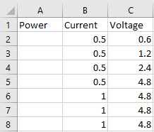
Теперь переберём все строки в нашей таблице, чтобы вычислить и вставить значения мощности, умножив ток на напряжение:
Как только это будет сделано, мы используем рассчитанные значения мощности, чтобы сгенерировать линейную диаграмму, которая будет вставлена в указанную ячейку, код показан ниже:
 Автоматически созданная таблица Excel
Извлечение диаграммы
Теперь, когда мы сгенерировали нашу диаграмму, нам нужно извлечь её как изображение, чтобы мы могли использовать её в нашем отчёте Word. Сначала укажем точное местоположение файла Excel, а также место, где должно быть сохранено изображение диаграммы:
Затем откройте электронную таблицу, используя следующий метод:
Позднее вы сможете перебирать все объекты диаграммы в электронной таблице (если их несколько) и сохранять их в указанном месте:
Автоматизация Microsoft Word
Теперь, когда у нас есть сгенерированное изображение диаграммы, мы должны создать шаблон документа, который в принципе является обычным документом Microsoft Word (.docx), сформированным именно так, как мы хотим: отчёт содержит шрифты, размеры шрифтов, структуру и форматирование страниц.
Теперь всё, что нам нужно сделать, — создать плейсхолдеры для сгенерированного нами контента, то есть табличные значения и изображения, и объявить их с именами переменных, как показано ниже.
 Шаблон документа Microsoft Word
Любой сгенерированный контент, включая текст и изображения, может быть объявлен в двойных фигурных скобках << variable_name >>. В случае таблиц вам нужно создать таблицу со строкой шаблона со всеми включёнными столбцами, затем нужно добавить одну строку вверху и одну строку ниже со следующей нотацией:
На рисунке выше — имена переменных:
table_contents для словаря Python, в котором будут храниться наши табличные данные;
Index для ключей словаря (первый столбец);
Power, Current и Voltage для значений словаря (второй, третий и четвёртый столбцы).
Затем импортируем наш шаблонный документ в Python и создаём словарь, в котором будут храниться значения нашей таблицы:
Далее импортируем ранее созданное в Excel изображение диаграммы и создадим другой словарь для создания экземпляров всех объявленных в документе шаблона переменных-заполнителей:
И, наконец, визуализируем отчёт с нашей таблицей значений и изображением диаграммы:
Результаты
И вот — автоматически сгенерированный отчёт Microsoft Word с числами и созданной в Microsoft Excel диаграммой. Мы получили полностью автоматизированный конвейер, его можно использовать, чтобы создать столько таблиц, диаграмм и документов, сколько вам потребуется.
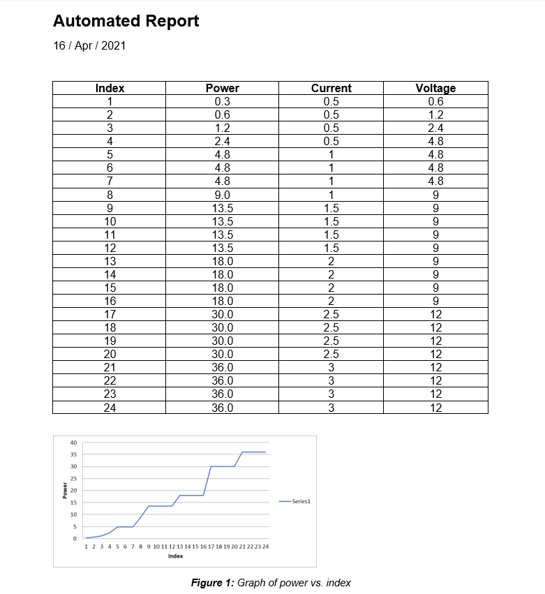 Автоматически сгенерированный отчёт
Исходный код
Вот мой репозиторий на GitHub с шаблоном документа и исходным кодом для этого туториала. А вот ссылка на курс Fullstack-разработчик на Python, который сделает из вас настоящего универсального солдата от кодинга.

Узнайте, как прокачаться и в других специальностях или освоить их с нуля:
Источник
How to Insert Excel Data Into Word (Tables, Files, Spreadsheets)
Microsoft Word is great for working on documents—but not so great with tables of data.
If you want to put a table into a Microsoft Word document, you can work with Word’s built-in table tools, or you can insert data directly from Excel.
Guess which one is better?
Getting your Excel data into Word is easy, makes it look better, and automatically updates. It’s a no-brainer💡
There are multiple ways of getting data from Excel into Word.
I’ll walk you through the best ones, step-by-step.
Please download my free sample workbook if you want to tag along.
Table of Contents
Free video on inserting Excel data in a Word document
Watch my video and learn how to easily copy and paste data from an Excel file to Word.
This video walked you through how to insert an Excel table in Word so it becomes a Microsoft Word table instead.
It’s done with all the classic copy-and-paste options: keep source formatting, match destination styles,
But there are other ways of getting things from Excel to Word.
Let’s dive into those below 🤿
What is an Excel Worksheet object?
Recent versions of Microsoft Office include the capability to insert objects into documents. These objects are either embedded or linked.
Embedded objects don’t update. If you include an embedded Excel object and change data in the Excel sheet you copied it from, no changes will be applied.
Linked objects update automatically. A linked Excel object will update to reflect changes in the original Excel sheet.
You can embed and link things other than Excel worksheets, but we’ll focus on Excel objects here.
It’s worth noting that the linked spreadsheet needs to remain available for this to work.
Also, this process works in reverse, as well: you can link to Word document objects from an Excel spreadsheet and insert them there in a matter of seconds.
Embedding Excel objects in Word
We’ll start with the simpler of the two: embedding an Excel object. Let’s take a look at the example workbook to see how it works.
Open the example workbook and a blank Word document.
On the first worksheet in the Excel file, you’ll see a small table. Select and copy it.

Go to your Word document, and paste the table with Ctrl + V.
You’ll see a table like this one:

If you click into this table, nothing notable will happen—you can edit the names of the months or the numbers, and they’ll change.
If you try inputting an Excel formula, however, it will only display as text.
Head back to the Excel worksheet and copy the table again.
In Word, click the Home tab of the Ribbon, and select Paste > Paste Special. In the resulting pop-up window, click on the Worksheet Object, and click OK.

You’ll now see a table that looks a bit different:

At first, it looks like the distinguishing feature of this table is gridlines.
But if you double-click the table, you’ll get a surprising new interface:

As you can see, this gives you an embedded version of Excel within Microsoft Word.
All because it’s a linked object. Pretty cool, huh?😎
You can do all the things you’re used to in Excel: use and edit formulas, apply conditional formatting, add new rows and columns, sort and filter data, and everything else you’ve come to expect from Excel.
And source formatting (from the Excel worksheet) is transferred to the Word document.
In short, it gives you a lot more table-editing power than you get with the standard Microsoft Word interface.
To exit the Excel interface, click outside of the table, and you’ll go back to the regular editor for your document.
If you go back to the Excel spreadsheet and make an edit in the table, you’ll see that the Excel object doesn’t update. So if your calculations change, or you get new data and add it to the spreadsheet, you’ll need to update your Word document manually.
Linking Excel objects in Word
As I mentioned before, embedded objects don’t automatically update. Linked objects, on the other hand, do.
And this can save you a lot of time.
Fortunately, linking an Excel object in Microsoft Word is easy.
The example workbook we used previously is the source Excel file.
Copy the table from the example workbook, and head back to the Word file. Again, click Paste > Paste Special in the Home tab. Again, select Microsoft Excel Worksheet Object.
This time, however, you’ll need one more click. On the left side of the window, you’ll see two radio buttons. One says Paste, and the other says Paste Link. Click the button next to Paste Link:

After hitting OK, you’ll get another table in your Word document. This one looks the same as the previous one:

There’s an important difference, however ⚠️
Let’s go back to the original Excel file and change one of the values.
We’ll change May’s value from 9 to 10.
Here’s what happens:

It might not be super clear in the GIF above, but the linked table automatically updates to match the Excel spreadsheet, while the embedded table doesn’t.
In other words, the Excel file changes are automatically applied to the Word document.
Insert an Excel worksheet in a Word document
Linking an Excel worksheet is the best way to get Excel data into Word because Excel is the best tool for working with spreadsheets.
If you want to insert a new object, you can insert a new spreadsheet into your Word document and work on it with the in-Word Excel tool.
To be completely honest, I don’t understand why you wouldn’t just work in Excel first, but I thought you might want to know anyway!
To insert a blank Excel worksheet object into the Word file, go to the Insert tab on the Ribbon.
Click the Object button in the Text group, then find the Microsoft Excel Worksheet object option.
This opens up the trusty ol’ object dialog box.

Hit OK, and you’ll get a blank worksheet in your Word document.
When you want to edit it, double-click the worksheet and you’ll open the Excel editor right inside of Word.

As before, you can do all the things you usually do in Excel right from Word in this worksheet.
And that’s an easy way of getting data from Excel to Word by making it an embedded object in the Word doc.
Источник
Excel is a great tool for doing all the analysis and finalizing the report. But sometimes, calculation alone cannot convey the message to the reader because every reader has their way of looking at the report. Some people can understand the numbers just by looking at them, some need some time to get the real story, and some cannot understand. So, they need a full and clear-cut explanation of everything.
You can download this Text in Excel Formula Template here – Text in Excel Formula Template
To bring all the users to the same page while reading the report, we can add text comments to the formula to make the report easily readable.
Let us look at how we can add text in Excel formulas.
Table of contents
- Formula with Text in Excel
- #1 – Add Meaningful Words Using with Text in Excel Formula
- #2 – Add Meaningful Words to Formula Calculations with TIME Format
- #3 – Add Meaningful Words to Formula Calculations with Date Format
- Things to Remember Formula with Text in Excel
- Recommended Articles
#1 – Add Meaningful Words Using Text in Excel Formula
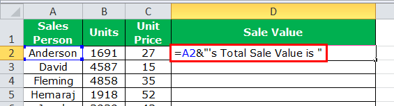
Often in Excel, we only perform calculations. Therefore, we are not worried about how well they convey the message to the reader. For example, take a look at the below data.
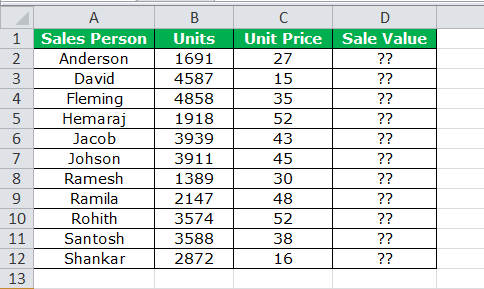
By looking at the above image, it is very clear that we need to find the sale value by multiplying Units to Unit PriceUnit Price is a measurement used for indicating the price of particular goods or services to be exchanged with customers or consumers for money. It includes fixed costs, variable costs, overheads, direct labour, and a profit margin for the organization.read more.
Apply simple text in the Excel formula to get the total sales value for each salesperson.
Usually, we stop the process here itself.
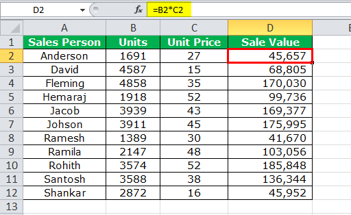
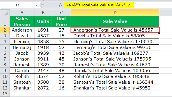
How about showing the calculation as Anderson’s total “Sale Value” is 45,657?
It looks like a complete sentence to convey a clear message to the user. So, let us go ahead and frame a sentence along with the formula.
So, let us go ahead and frame a sentence along with the formula.
- We know the format of the sentence to be framed. Firstly, we need a “Sales Person” name to appear. So, we must select the cell A2 cell.

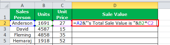
- Now, we need “Total Sale Value” after the salesperson’s name. We need to put the ampersand operator sign after selecting the first cell to comb this text value.

- Now, we need to do the calculation to get the sale value. Put on more (ampersand) sign and apply the formula as B*C2.

- Now, we must press the “Enter” key to complete the formula and our text values.

One problem with this formula is that sales numbers are not formatted properly. Because they do not have a thousand separators, that would have made the numbers look properly.
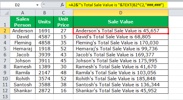
There is nothing to worry about; we can format the numbers with the TEXT function in the Excel formula.
Edit the formula. As shown below, the calculation part applies the Excel TEXT function to format the numbers.

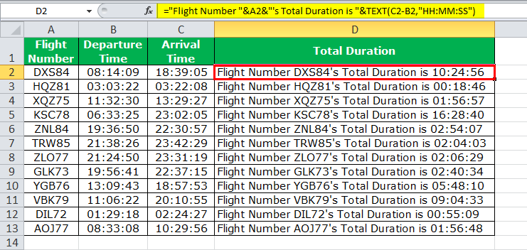
Now, we have the proper format of numbers along with the sales values. The TEXT function in Excel formula format the calculation (B2*C2) to the format of ###, ###.
#2 – Add Meaningful Words to Formula Calculations with TIME Format
We have seen how to add text values to our formulas to convey a clear-cut message to the readers or users. Now, we will be adding text values to another calculation, which includes time calculations.
We have data on flight departure and arrival timings. We need to calculate the total duration of each flight.
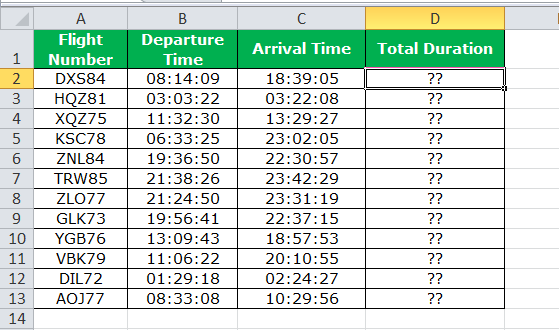
Not only the total duration, but we want to show the message like this “Flight Number DXS84’s total duration is 10:24:56.”
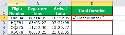
In cell D2, we must start the formula. Our first value is “Flight Number.” We must enter this in double-quotes.
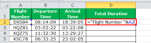
The next value we need to add is the flight number already in cell A2. Enter the “&” symbol and select cell A2.
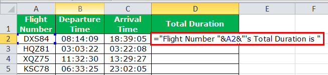
The next thing we need to add to the text‘s “Total Duration.”We must insert one more “&”symbol and enter this text in double-quotes.
Now comes the most important part of the formula. We need to calculate the total duration after “&” the symbol enters the formula as C2 – B2.
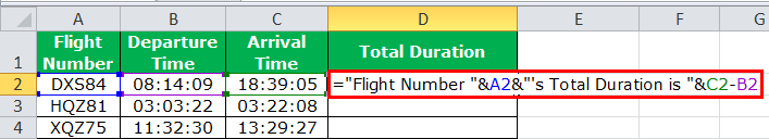
Our full calculation is complete. Press the “Enter” key to get the result.
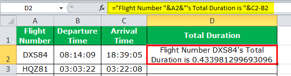
We got the total duration as 0.433398, which is not in the right format. So, we must apply the TEXT function to perform the calculation and format that to TIME.
#3 – Add Meaningful Words to Formula Calculations with Date Format
The TEXT function can perform the formatting task when adding text values to get the correct number format. Now, we will see it in the date format.
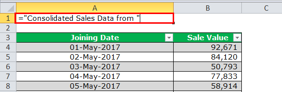
Below is the daily sales table that we update the values regularly.
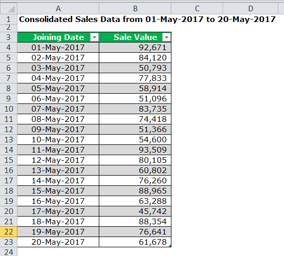
We need to automate the heading as the data keeps adding, i.e., we should change the last date as per the last day of the table.
Step 1: We must first open the formula in the A1 cell as “Consolidated Sales Data from.”
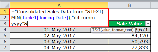
Step 2: Put the “&” symbol and apply the TEXT function in the Excel formula. Apply the MIN function to get the least date from this list inside the TEXT function. And format it as “dd-mmm-yyyy.”
Step 3: Now, enter the word to.
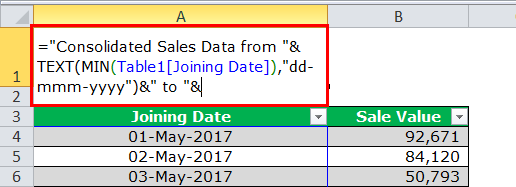
Step 4: To get the latest date from the table, we must apply the MAX formulaThe MAX Formula in Excel is used to calculate the maximum value from a set of data/array. It counts numbers but ignores empty cells, text, the logical values TRUE and FALSE, and text values.read more, and format it as the date by using TEXT in the Excel formula.
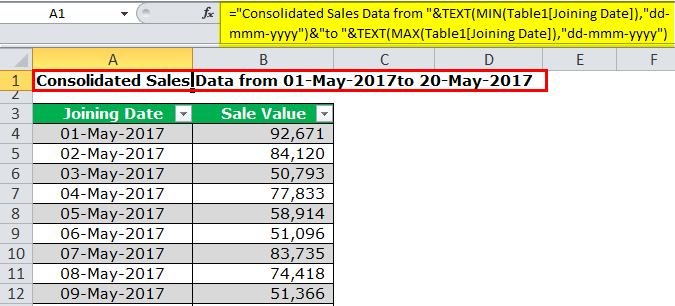
As we update the table, it will automatically update the heading.
Things to Remember Formula with Text in Excel
- We can add the text values according to our preferences by using the CONCATENATE function in excelThe CONCATENATE function in Excel helps the user concatenate or join two or more cell values which may be in the form of characters, strings or numbers.read more or the ampersand (&) symbol.
- To get the correct number format, we must use the TEXT function and specify the number format we want to display.
Recommended Articles
This article has been a guide on Text in Excel Formula. Here, we discuss how to add text in the Excel formula cell along with practical examples and downloadable Excel templates. You may also look at these useful functions in Excel: –
- Separate Text in Excel
- How to Wrap Text in Excel?
- How to Convert Text to Numbers in Excel?
- Convert Date to Text in Excel
![]()
Download Article
![]()
Download Article
An Excel document can be overwhelming to look through. Thankfully, you can use the search function to conveniently locate a particular word, or group of words, in an Excel worksheet.
-

1
Launch MS Excel. Do this by clicking on its icon in your desktop. It is the green X icon with spreadsheets in its background.
- If you don’t have an Excel shortcut icon on your desktop, find it in your Start menu and click the icon there.
-
2
Find the Excel file you want to open. Click “File” in the upper left corner of the window then click “Open.” A file browser will appear. Browse your computer for the Excel file you want to open.
Advertisement
-
3
Open the file. Once you’ve located the file, click on it to select then click “Open” in the lower-right portion of the file browser.


Advertisement
-
1
Click a cell. Once you’re in the worksheet, click on any cell on the worksheet to ensure that the window is active.
-
2
Open the Find/Replace With window. Hit the key combination Ctrl + F on your keyboard. A new window will appear with two fields: “Find” and “Replace with.”
-
3
Type in the words you want to find. Enter the exact word or phrase you want to search for, and click on the “Find” button in the lower right of the Find window.
- Excel will begin searching for matches of the word, or words, you entered in the search field. All words in the document that matches those you entered will be highlighted to help you better locate them.


Advertisement
Ask a Question
200 characters left
Include your email address to get a message when this question is answered.
Submit
Advertisement
Thanks for submitting a tip for review!
About This Article
Thanks to all authors for creating a page that has been read 91,003 times.
Is this article up to date?
Excel for Microsoft 365 Excel for Microsoft 365 for Mac Excel for the web Excel 2021 Excel 2021 for Mac Excel 2019 Excel 2019 for Mac Excel 2016 Excel 2016 for Mac Excel 2013 Excel 2010 Excel 2007 Excel for Mac 2011 Excel Starter 2010 More…Less
To get detailed information about a function, click its name in the first column.
Note: Version markers indicate the version of Excel a function was introduced. These functions aren’t available in earlier versions. For example, a version marker of 2013 indicates that this function is available in Excel 2013 and all later versions.
|
Function |
Description |
|---|---|
|
ARRAYTOTEXT function |
Returns an array of text values from any specified range |
|
ASC function |
Changes full-width (double-byte) English letters or katakana within a character string to half-width (single-byte) characters |
|
BAHTTEXT function |
Converts a number to text, using the ß (baht) currency format |
|
CHAR function |
Returns the character specified by the code number |
|
CLEAN function |
Removes all nonprintable characters from text |
|
CODE function |
Returns a numeric code for the first character in a text string |
|
CONCAT function |
Combines the text from multiple ranges and/or strings, but it doesn’t provide the delimiter or IgnoreEmpty arguments. |
|
CONCATENATE function |
Joins several text items into one text item |
|
DBCS function |
Changes half-width (single-byte) English letters or katakana within a character string to full-width (double-byte) characters |
|
DOLLAR function |
Converts a number to text, using the $ (dollar) currency format |
|
EXACT function |
Checks to see if two text values are identical |
|
FIND, FINDB functions |
Finds one text value within another (case-sensitive) |
|
FIXED function |
Formats a number as text with a fixed number of decimals |
|
LEFT, LEFTB functions |
Returns the leftmost characters from a text value |
|
LEN, LENB functions |
Returns the number of characters in a text string |
|
LOWER function |
Converts text to lowercase |
|
MID, MIDB functions |
Returns a specific number of characters from a text string starting at the position you specify |
|
NUMBERVALUE function |
Converts text to number in a locale-independent manner |
|
PHONETIC function |
Extracts the phonetic (furigana) characters from a text string |
|
PROPER function |
Capitalizes the first letter in each word of a text value |
|
REPLACE, REPLACEB functions |
Replaces characters within text |
|
REPT function |
Repeats text a given number of times |
|
RIGHT, RIGHTB functions |
Returns the rightmost characters from a text value |
|
SEARCH, SEARCHB functions |
Finds one text value within another (not case-sensitive) |
|
SUBSTITUTE function |
Substitutes new text for old text in a text string |
|
T function |
Converts its arguments to text |
|
TEXT function |
Formats a number and converts it to text |
|
TEXTAFTER function |
Returns text that occurs after given character or string |
|
TEXTBEFORE function |
Returns text that occurs before a given character or string |
|
TEXTJOIN function |
Combines the text from multiple ranges and/or strings |
|
TEXTSPLIT function |
Splits text strings by using column and row delimiters |
|
TRIM function |
Removes spaces from text |
|
UNICHAR function |
Returns the Unicode character that is references by the given numeric value |
|
UNICODE function |
Returns the number (code point) that corresponds to the first character of the text |
|
UPPER function |
Converts text to uppercase |
|
VALUE function |
Converts a text argument to a number |
|
VALUETOTEXT function |
Returns text from any specified value |


Important: The calculated results of formulas and some Excel worksheet functions may differ slightly between a Windows PC using x86 or x86-64 architecture and a Windows RT PC using ARM architecture. Learn more about the differences.
See Also
Excel functions (by category)
Excel functions (alphabetical)
Need more help?
A while back Vernon asked me how he could search one cell and compare it to a list of words. If any of the words in the list existed then return the matching word.
Ugh, I’ve written that 3 times and I’m not sure it’s any clearer…let’s look at an example.
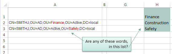
I’ve highlighted the matching words in column A red.
What we want Excel to do is to check the text string in column A to see if any of the words in our list in H1:H3 are present, if they are then return the matching word. Note: I’ve given cells H1:H3 the named range ‘list’.
There are a few ways we can tackle this so let’s take a look at our options.
Warning: this is quite an advanced topic which requires an array formula to solve it.
Update: It’s easier and more robust to use Power Query to search for text strings, including case and non-case sensitive searches.
Non-Case Sensitive Matching
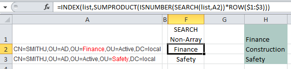
If you aren’t worried about case sensitive matches then you can use the SEARCH function with INDEX, SUMPRODUCT and ISNUMBER like this:
=INDEX(list,SUMPRODUCT(ISNUMBER(SEARCH(list,A2))*ROW($1:$3)))
In English our formula reads:
SEARCH cell A2 to see if it contains any words listed in cells H1:H3 (i.e. the named range ‘list’) and return the number of the character in cell A2 where the word starts. Our formula becomes:
=INDEX(list,SUMPRODUCT(ISNUMBER({20;#VALUE!;#VALUE!})*ROW($1:$3)))
i.e. in cell A2 the ‘F’ in the word ‘Finance’ starts in position 20.
Now using ISNUMBER test to see if the SEARCH formula returns any numbers (if it does it means there is a match). ISNUMBER will return TRUE if there is a number and FALSE if not (this gives us a list of Boolean TRUE or FALSE values). Our formula becomes:
=INDEX(list,SUMPRODUCT({TRUE;FALSE;FALSE}*ROW($1:$3)))
Use the ROW function to return an array of numbers {1;2;3} (see notes below on why I’ve used ROW in this formula). Our formula becomes:
=INDEX(list,SUMPRODUCT({TRUE;FALSE;FALSE}*{1;2;3}))
When you multiply Boolean TRUE/FALSE values they become their numeric equivalents i.e. TRUE = 1 and FALSE = 0. So our formula evaluates this ({TRUE;FALSE;FALSE}*{1;2;3}) like so: {1*1, 0*2, 0*3} and our formula becomes:
=INDEX(list,SUMPRODUCT({1;0;0}))
SUMPRODUCT simply sums the values {1+0+0} which gives us 1. Note: by using SUMPRODUCT we are avoiding the need for an array formula that requires CTRL+SHIFT+ENTER. Our formula becomes:
=INDEX(list,1)
Index can now go ahead and return the 1st value in the range of cells H1:H3 which is ‘Finance’.
Note: the above formula will not work if a match isn’t found. If you want to return an error if a match isn’t found then you can use this variation:
=INDEX(list,IF(SUMPRODUCT(--ISNUMBER(SEARCH(list,A2)))<>0,SUMPRODUCT(ISNUMBER(SEARCH(list,A2))*ROW($1:$3)),NA()))
Not as elegant, is it? In which case you might prefer one of the array formulas below.
Notes about the ROW Function:
The ROW function simply returns the row number of a reference. e.g. ROW(A2) would return 2. When used in an array formula it will return an array of numbers. e.g. ROW(A2:A4) will return {2;3;4}. We can also give just the row reference(s) to the ROW function like so ROW(2:4).
In this formula we have used ROW to simply return an array of values {1;2;3} that represent the items in our ‘list’ i.e. Finance is 1, Construction is 2 and Safety is 3. Alternatively we could have typed {1;2;3} direct in our formula, or even referenced the named range like this ROW(list).
So you see using the ROW function is just a quick and clever way to generate an array of numbers.
What you must bear in mind when using the ROW function for this purpose is that we need a list of numbers from 1 to 3 because there are 3 words in our list and we’re trying to find the position of the matching word.
In this example the formula; ROW(list) will also work because our list happens to start on row 1 but if we were to start ‘list’ on row 2 we would come unstuck because ROW(list) would return {2;3;4} i.e. ‘list’ would actually reference cells H2:H4.
So, don’t get confused into thinking the ROW part of the formula is simply referencing the list or range of cells where the list is, the important point is that the ROW formula returns an array of numbers and we’re using those numbers to represent the number of rows in the ‘list’ which must always start with 1.
Functions Used
INDEX
SEARCH or FIND
ISNUMBER
SUMPRODUCT
ROW — Explained above.
Case Sensitive Matching
[updated Dec 5, 2013]
If your search is case sensitive then you not only need to replace SEARCH with FIND, but you also need to introduce an IF formula like so:
=INDEX(list,IF(SUMPRODUCT(ISNUMBER(FIND(list,A2))*ROW($1:$3))<>0,SUMPRODUCT(ISNUMBER(FIND(list,A2))*ROW($1:$3)),NA()))
Unfortunately it’s not as simple or elegant as the first non-case sensitive search. Instead the array formulas below are nicer
Array Formula Options
Below are some array formula options to achieve the same result. They use LARGE instead of SUMPRODUCT, and as a result you need to enter these by pressing CTRL+SHIFT+ENTER.
Non-case Sensitive:
[updated Dec 5, 2013]
=INDEX(list,LARGE(IF(ISNUMBER(SEARCH(list,A2)),ROW($1:$3)),1)) Press CTRL+SHIFT+ENTER
Case sensitive:
[updated Dec 5, 2013]
=INDEX(list,LARGE(IF(ISNUMBER(FIND(list,A2)),ROW($1:$3)),1)) Press CTRL+SHIFT+ENTER
Download
Enter your email address below to download the sample workbook.
By submitting your email address you agree that we can email you our Excel newsletter.
Thanks
Special thanks to Roberto for suggesting the ‘updated’ formulas above.