
Any database (DB) is a summary table with the parameters and information. Most schools programs included the creation of a database in Microsoft Access. But Excel gives all the opportunities to build simple databases and easily navigate through them.
How to make the database in Excel so it was convenient not to only store but also process the data: generate reports, build charts, graphs, etc.
Step by step to create a database in Excel
At first we will learn how to create a database using Excel tools. Let’s imagine that we are the shop. We draw up a summary table of data with various products deliveries from different suppliers.
| № | Product | Product Category | Quantity | Price kg | Total value | Delivery month | Supplier | Who accepted items |
We puzzled out with headlines. Now fill the table. We start with a serial number. We don’t have to put down the numbers manually. Enter in cells A4 and A5 one and two respectively. Then select those two cells with left mouse button and grab the corner of the segregation and extend down to any number of rows. In a small little window you will see the final number.
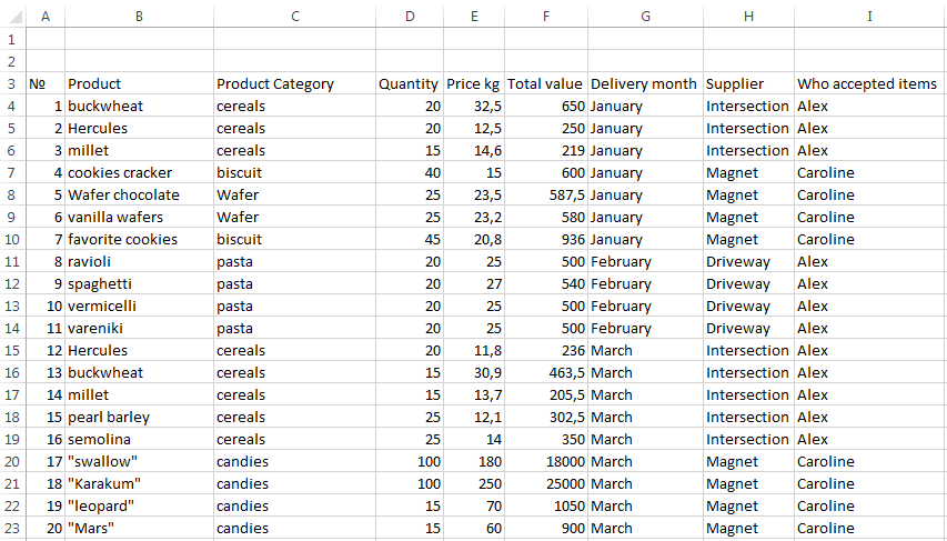
Note. This table can be downloaded at the end of the article.
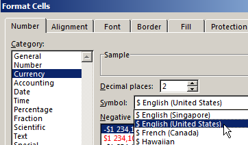
Base show us that some of the information will be presented in text form (product, category, month, etc.), and some is in the financial. Select the cells with the headlines named Price kg and Total value E4:F23. Use right-click to see context menu where choose «Format Cells» CTRL+1.
A window will appear where we will choose the Currency format. Enter the number of decimal places equals 1. We don’t have to choose designation because in the header we already pointed out that the price and value in $ English (United States).
Similarly we proceed with the cells where the quantity column will be filled. Select numerical number.
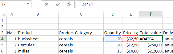
Let’s deal with another preparatory action. You can immediately use that fact that in the corresponding cells value is calculated as the price multiplied by the quantity. To make this we enter in cell F4 formula and stretch it to the other cells in this column. Thus the cost will be calculated automatically while filling the table.
Now fill the table with data.
It’s important! It is necessary to stick to a single style of writing while filling the cells. If the original name of the employee is recorded as Alex AA, then the rest cells should be filled similarly. The work with the database will be difficult if somewhere name will be written differently, for example, Alexey Alex.
The table is ready. In reality it may be much longer. We have added a several positions for example. Let us give the database a more aesthetic appearance with making the frame. To do this select the entire table and find the parameter «All Borders» on the panel.
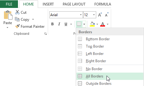
Similarly, frame the headlines thick outer boundary.
Excel functions for working with database
Now we turn to the functions that Excel offers to work with the database.
Working with databases in Excel
Example: we want to know all the products receipted by Alex AA Theoretically, you can run through the all rows visually where this name appears and then copy them to a separate table. But what if our database composed of several hundreds of items? FILTER comes to help us.
Select all the headlines in the table and click «FILTER» in the «DATA» tab, (CTRL + SHIFT + L).
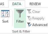
In each cell in the header appears black arrow on a gray background which can be clicked to filter the data. Click it in the parameter WHO ACCEPTED ITEMS and remove the check mark from the CAROLINE name.
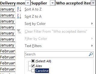
Thus there are remains data only with Alex.
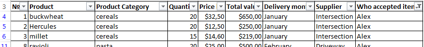
Note! When you are sorting data not only all the positions in the columns stays in its places but rows of numbers also corresponding to the sheet (these are highlighted in blue). This feature is useful to us later.
You can make additional filtering. Determine which kind of grouts Alex accepted. Click the arrow on the cell PRODUCT CATEGORIY and leave only grouts.
If you need to return the full database you can make it in easiest way: set out all the checkboxes in the corresponding filters.
Data sorting
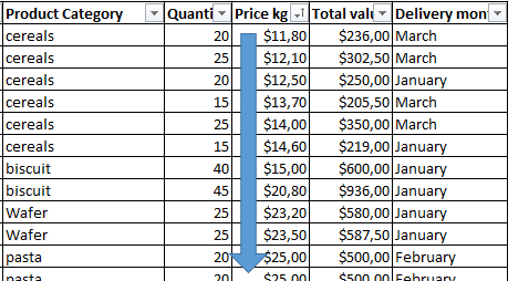
In this example the database was filled in chronological order during the supplying goods in the shop. But if we want to sort the data on a different principle excel allows you to do that too.
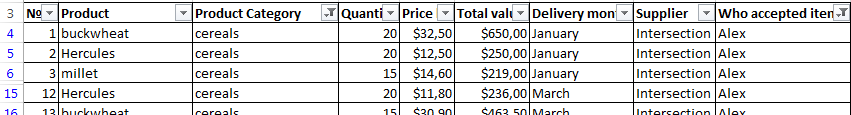
For example, we want to sort the products as price increase. Those the first line will be the cheapest product and in the last will be the most expensive. Select the column with the price and on the HOME tab and choose the «Sort & Filter».
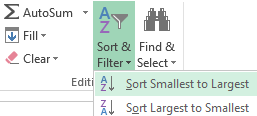
As we decided that lower price would be on top choose «Sort Smallest to Largest». You will see another window where we select «Expand the selection», so the other columns can also adjust to the sorting.
We see that the data is sorted in order to increasing price.
Note! You can make sorting in order to increase or decrease parameter using AutoFilter. Such action is also proposed when you press the arrow.
Sort by condition
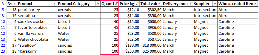
We need to extract from the database products that were purchased in lots of 25 kg or more. For this purpose click the filter arrow on QUANTITY cell, and select the following options.
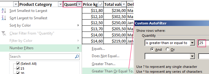
In the window that appears in front of condition БОЛЬШЕ ИЛИ РАВНО inscribe number 25. Then you will get sample indicating the products ordered by the lots greater than 25 kg or equal to this. Those products also sorted in the manner of its price growth since we did not remove sorting by price.
Subtotals
This is another useful function which allows calculating the sum, the multiplication, minimum or average value, etc. using the existing database. It is called the subtotals. =SUBTOTAL() This function has one main advantage. It allows making calculations with certain function even if you change the size of the table. Let’s consider it with an example.
Let us give our full database suitable view. Next we create a formula for the AutoSum in column Total value. Enter formula writing it in the F26 cell. At the same time remember how database sorting in Excel: number of rows fixed in place. Therefore the formula will still be in the F26 cell even when we do filtering.
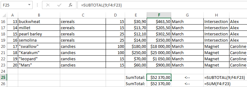
Subtotal function has 30 arguments. The first is static: the action code. By default Excel set code number 9, so let it be. The second and subsequent arguments are dynamic: this is links to ranges which are summed up. We have a range: F4: F24. It turned out 19,670 rubles.
Now try again to sort number, leaving only a party of 25 kg and >.
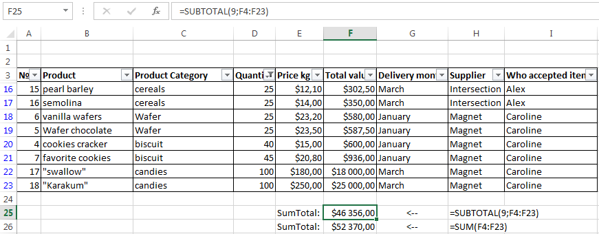
We see that the amount has changed, too.
download example
In Excel, you can also create a small database and easy to work with them. When large volumes of data is very convenient and efficient.
Do you need to create and use a database? This post is going to show you how to make a database in Microsoft Excel.
Excel is the most common data tool used in businesses and personal productivity across the world.
Since Excel is so widely used and available, it tends to get used frequently to store and manage data as a makeshift database. This is especially true with small businesses since there is no budget or expertise available for more suitable tools.
This post will show you what a database is and the best practices you should follow if you’re going to try and use Excel as a database.

Get the example files used in this post with the above link and follow along below!
What is a Database?
A database is a structured set of data that is often in an electronic format and is used to organize, store. and retrieve data.
For example, a database might be used to store customer names, addresses, orders, and product information.
Databases often have key features that make them an ideal place to store your data.
Database vs Excel
An Excel spreadsheet is not a database, but it does have a lot of great and easy-to-use features for working with data.
Here are some of the key features of a database and how they compare to an Excel file.
| Feature | Database | Excel |
|---|---|---|
| Create, read, update, and delete records | ✔️ | ✔️ Excel allows anyone to add or edit data. This can be viewed as a negative consideration. |
| Data types | ✔️ | ⚠️ Excel allows for simple data types such as text, numbers, dates, boolean, images, and error values. But lacks more complex data types such as date and timezones, files, or JSON. |
| Data validation | ✔️ | ⚠️ Excel has some data validation features, but you can only apply one rule at a time and these can easily be overridden on purpose or by accident. |
| Access and security | ✔️ | ❌ Excel doesn’t have any access or security controls. This is usually managed through your on-premise network or through SharePoint online. But anyone can access your Excel file if it’s downloaded and sent to them. |
| Version control | ✔️ | ❌ Excel has no version control. This can be managed through SharePoint. |
| Backups | ✔️ | ❌ Excel has no automated backups. These can be manually created or automated in SharePoint. |
| Extract and query data | ✔️ | ✔️ Excel allows you to extract and query data through Power Query which is easy to learn and use. |
| Perform calculations | ✔️ | ✔️ Excel has a large library of functions that can be used in calculated columns inside tables. Excel also has the DAX formula language for calculated columns in Power Pivot. |
| Aggregate and summarize data | ✔️ | ✔️ Excel can easily aggregate and summarize data with formulas, pivot tables, or power pivots. |
| Relationships | ✔️ | ✔️ Excel has many lookup functions such as XLOOKUP, as well as table merge functionality in Power Query, and 1 to many relationships in Power Pivot. |
| Scale with large amounts of data | ✔️ | ⚠️ Excel can hold up to 1,048,576 rows of data in a single sheet. Tools like Power Query and Power Pivot can help you deal with larger amounts of data but they will be constrained based on your hardware specifications. |
| User friendly | ❌ A database might not be user-friendly and may come with a steep learning curve that your intended users won’t be able to handle. | ✔️ Most people have some experience with using Excel. |
| Cost | ❌ Can be expensive to set up, run, and maintain a proper database tool. | ✔️ Your organization might already have access to and use Excel. |
This is not a comprehensive list of features that a database will have, but they are some of the major features that will usually make a proper database a more suitable option.
The features that a database has depends on what database it is. Not all databases have the same features and functionality.
You will need to decide what features are essential for your situation in order to decide if you should use Excel or some other database tool.
💡 Tip: If you have Excel for Microsoft 365, then consider using Dataverse for Teams as your database instead of Excel. Dataverse has many of the great database features mentioned above and it is included in your Microsoft 365 license at no additional cost.
Relational Database Design
A good deal of thought should happen about the structure of your database before you begin to build it. This can save you a lot of headaches later on.
Most databases have a relational design. This means the database contains many related tables instead of one table that contains all the data.
Suppose you want to track orders in your database.
One option is to create a single flat table that contains all the information about the order, the products, and the customer that created the order.
This isn’t very efficient as you end up creating multiple entries of the same customer information such as name, email, and address. You can see in the above data, column G, H, and I contains a lot of duplicate values.
A better option is to create separate tables to store the Order, Product, and Customer data.
The Order data can then reference a unique identifier in the Product and Customer data that will relate the tables and avoid unnecessary duplicate data entry.
This same example data might look like this when reorganized into multiple related tables.
- An Orders table that contains the Item and Customer ID field.
- A Products table that relates to the Item fields in the Orders table.
- A Customers table that relates to the Customer ID in the Orders table.
This avoids duplicated data entry in a flat single table structure and you can use the Item or Customer ID unique identifier to look up the related data in the respective Products or Customers tables.
Tabular Data Structure in Excel
If you’re going to use Excel as your database, then you’re going to need your data in tabular format. This refers to the way the data is structured.
The above example shows a product order dataset in tabular format. A tabular data format is best suited for Excel due to the row and column structure of a spreadsheet.
Here are a few rules your data should follow so that it’s in tabular format.
- 1st row should contain column headings. This is just a short and descriptive name for the data contained below.
- No blank column headings. Every column of data should have a name.
- No blank columns or blank rows. Blank values within a field are ok, but columns or rows that are entirely blank should be removed.
- No subtotals or grand totals within the data.
- One row should represent exactly one record of data.
- One column should contain exactly one type of data.
In the above orders example data, you can see B2:E2 contains the column headings of an Order ID, Customer ID, Order Date, Item, and Quantity.
The dataset has no blank rows or columns, and no subtotals are included.
Each row in the dataset represents an order for one type of product.
You’ll also notice each column contains one type of data. For example, the Item column only contains information on the name of the product and does not include other product information such as the price.
⚠️ Warning: If you don’t adhere to this type of structure for your data, then summarizing and analyzing your data will be more difficult later. Tools such as pivot tables require tabular data!
Use Excel Tables to Store Data
Excel has a feature that is specifically for storing your tabular data.
An Excel Table is a container for your tabular datasets. They help keep all the same data together in one object with many other benefits.
💡 Tip: Check out this post to learn more about all the amazing features of Excel Tables.
You will definitely want to use a table to store and organize any data table that will be a part of your dataset.
How to Create an Excel Table
Follow these steps to create a table from an existing set of data.
- Select any cell inside your dataset.
- Go to the Insert tab in the ribbon.
- Select the Table command.
This will open the Create Table menu where you will be able to select the range containing your data.
When you select a cell inside your data before using the Table command, Excel will guess the full range of your dataset.
You will see a green dash line surrounding your data which indicates the range selected in the Create Table menu. You can click on the selector button to the right of the range input to adjust this range if needed.
- Check the My table has headers option.
- Press the OK button.
📝 Note: The My table has headers option needs to be checked if the first row in your dataset contains column headings. Otherwise, Excel will create a table with generic column heading titles.
Your Excel data will now be inside a table! You will immediately see that it’s inside a table as Excel will apply some default format which will make the table range very obvious.
💡 Tip: You can choose from a variety of format options for your table from the Table Design tab in the Table Styles section.
The next thing you will want to do with your table is to give it a sensible name. The table name will be used to reference the table in formulas and other tools, so giving it a short descriptive name will help you later when reading formulas.
- Go to the Table Design tab.
- Click on the Table Name input box.
- Type your new table name.
- Press the Enter key to accept the new name.
Each table in your database will need to be in a separate table, so you will need to repeat the above process for each.
How to Add New Data to Your Table
You will likely need to add new records to your database. This means you will need to add new rows to your tables.
Adding rows to an Excel table is very easy and you can do it a few different ways.
You can add new rows to your table from the right-click menu.
- Select a cell inside your table.
- Right-click on the cell.
- Select Insert from the menu.
- Select Table Rows Above from the submenu.
This will insert a new blank row directly above the selected cells in your table.
You can add a blank row to the bottom of your table with the Tab key.
- Place the active cell cursor in the lower right cell of the table.
- Press the Tab key.
A new blank row will be added to the bottom of the table.
But the easiest way to add new data to a table is to type directly below the table. Data entered directly underneath the table is automatically absorbed into the table!
Excel Workbook Layout
If you are going to create an Excel database, then you should keep it simple.
Your Excel database file should contain only the data and nothing else. This means any reports, analysis, data visualization, or other work related to the data should be done in another Excel file.
Your Excel database file should only be used for adding, editing, or deleting the data stored in the file. This will help decrease the chance of accidentally changing your data, as the only reason to open the file will be to intentionally change the data.
Each table in the database should be stored in a separate worksheet and nothing else except the table should be in that sheet. You can then name the worksheet based on the table it contains so your file is easy to navigate.
💡 Tip: Place your table starting in cell A1 and then hide the remaining columns. This way it is clear the sheet should only contain the table and nothing else.
The only other sheet you might optionally include is a table of contents to help organize the file. This is where you can list each table along with the fields it contains and a description of what these fields are.
💡 Tip: You can hyperlink the table name listed in the table of contents to its associated sheet. Select the name and press Ctrl + K to create a hyperlink. This can help you navigate the workbook when you have a lot of tables in your database.
Use Data Validation to Prevent Invalid Data
Data validation is a very important feature for any database. This allows you to ensure only specific types of data are allowed in a column.
You might create data validation rules such as.
- Only positive whole numbers are entered in a quantity column.
- Only certain product names are allowed in the product column.
- A column can’t contain any duplicate values.
- Dates are between two given dates.
Excel’s data validation tools will help you ensure the data entered in your database follow such rules.
Follow these steps to add a data validation rule to any column in your table.
- Left-click on the column heading to select the entire column.
When you hover the mouse cursor over the top of your column heading in a table, the cursor will change to a black downward pointing arrow. Left-click and the entire column will be selected.
The data validation will automatically propagate to any new rows added to the table.
- Go to the Data tab.
- Click on the Data Validation command.
This will open up the Data Validation menu where you will be able to choose from various validation settings. If there is no active validation in the cell, you should see the Any values option selected in the Allow criteria.
Only Allow Positive Whole Number Values
Follow these steps from the Data Validation menu to allow only positive whole number values to be entered.
- Go to the Settings tab in the Data Validation menu.
- Select the Whole number option from the Allow dropdown.
- Select the greater than option from the Data dropdown.
- Enter 0 in the Minimum input box.
- Press the OK button.
💡 Tip: Keep the Ignore blank option checked if you want to allow blank cells in the column.
This will apply the validation rule to the column and when a user tries to enter any number other than 1, 2, 3, etc… they will be warned the data is invalid.
Only Allow Items from a List
Selecting items from a dropdown list is a great way to avoid incorrect text input such as customer or product names.
Follow these steps from the Data Validation menu to create a dropdown list for selecting text values in a column.
- Go to the Settings tab in the Data Validation menu.
- Select the List option from the Allow dropdown.
- Check the In-cell dropdown option.
- Add the list of items to the Source input.
- Press the OK button.
📝 Note: If you place the list of possible options inside an Excel Table and select the full column for the Source reference, then the range reference will update as you add items to the table.
Now when you select a cell in the column you will see a dropdown list handle on the right of the cell. Click on this and you will be able to choose a value from a list.
Only Allow Unique Values
Suppose you want to ensure the list of products in your Products table is unique. You can use the Custom option in the validation settings to achieve this.
- Go to the Settings tab in the Data Validation menu.
- Select the Custom option from the Allow dropdown.
=(COUNTIFS(INDIRECT("Products[Item]"),A2)=1)- Enter the above formula in the Formula input.
- Press the OK button.
The formula counts the number of times the current row’s value appears in the Products[Item] column using the COUNTIFS function.
It then determines if this count is equal to 1. Only values where the formula evaluates to 1 are allowed which means the product name can’t have been in the list already.
📝 Note: You need to reference the column by name using the INDIRECT function in order for the range to grow as you add items to your table!
Show Input Message when Cell is Selected
The data validation menu allows you to show a message to your users when a cell is selected. This means you can add instructions about what types of values are allowed in the column.
Follow these steps to add an input message in the Data Validation menu.
- Go to the Input Message tab in the Data Validation menu.
- Keep the Show input message when cell is selected option checked.
- Add some text to the Title section.
- Add some text to the Input message section.
- Press the OK button.
When you select a cell in the column which contains the data validation, a small yellow pop-up will appear with your Title and Input message text.
Prevent Invalid Data with Error Message
When you have a data validation rule in place, you will usually want to prevent invalid data from being entered.
This can be achieved using the error message feature in the Data Validation menu.
- Go to the Error Alert tab in the Data Validation menu.
- Keep the Show error alert after invalid data is entered option checked.
- Select the Stop option in the Style dropdown.
- Add some text to the Title section.
- Add some text to the Error message section.
- Press the OK button.
📝 Note: The Stop option is essential if you want to prevent the invalid data from being entered rather than only warning the user the data is invalid.
When you try to enter a repeated value in the column your custom error message will pop up and prevent the value from being entered in the cell.
Data Entry Form for Your Excel Database
Excel doesn’t have any fool-proof methods to ensure data is entered correctly, even when data validation techniques previously mentioned are used.
When a user copies and pastes or cuts and pastes values, this can override data validation in a column and cause incorrect data to enter into your database.
Using a data entry form can help to avoid data entry errors and there are a couple of different options available.
- Use a table for data entry.
- Use the quick access toolbar data entry form.
- Use Microsoft Forms for data entry.
- Use Microsoft Power Automate app for data entry.
- Use Microsoft Power Apps for data entry.
💡 Tip: Check out this post for more details on the various data entry form options for Excel.
Tools such as Microsoft Forms, Power Automate, and Power Apps will give you more data validation, access, and security controls over your data entry compared with the basic Excel options.
Access and Security for Your Excel Database
Excel isn’t a secure option for your data.
Whatever measures you set up in your Excel file to prevent users from changing data by accident or on purpose will not be foolproof.
Whoever has access to the file will be able to create, read, update, and delete data from your database if they are determined. There are also no options to assign certain privileges to certain users within an Excel file.
However, you can manage access and security to the file from SharePoint.
💡 Tip: Check out this post from Microsoft about recommendations for securing SharePoint files for more details.
When you store your Excel file in SharePoint you’ll also be able to see recent changes.
- Go to the Review tab.
- Click on the Show Changes command.
This will open up the Changes pane on the right-hand side of the Excel sheet.
It will show you a chronological list of all the recent changes in the workbook, who made those changes, when they made the change, and what the previous value was.
You can also right-click on a cell and select Show Changes. This will open the Changes pane filtered to only show the changes for that particular cell.
This is a great way to track down the cause of any potential errors in your data.
Query Your Excel Database with Power Query
Your Excel database file should only be used to add, edit, or delete records in your tables.
So how do you use the data for anything else such as creating reports, analysis, or dashboards?
This is the magic of Power Query! It will allow you to connect to your Excel database and query the data in a read-only manner. You can build all your reports, analysis, and dashboards in a separate file which can easily be refreshed with the latest data from your Excel database file.
Here’s how to use power query to quickly import your data into any Excel file.
- Go to the Data tab.
- Click on the Get Data command.
- Choose the From File option.
- Choose the From Excel Workbook option in the submenu.
This will open a file picker menu where you can navigate to your Excel database file.
- Select your Excel database file.
- Click on the Import button.
⚠️ Warning: Make sure your Excel database file is closed or the import process will show a warning that it’s unable to connect to the file because it’s in use!
Clicking on the Import button will then open the Navigator menu. This is where you can select what data to load and where to load it.
The Navigator menu will list all the tables and sheets in the Excel file. Your tables might be listed with a suffix on the name if you’ve named the sheets and tables the same.
- Check the option to Select multiple items if you want to load more than one table from your database.
- Select which tables to load.
- Click on the small arrow icon next to the Load button.
- Select the Load To option in the Load submenu.
This will open the Import Data menu where you can choose to import your data into a Table, PivotTable, PivotChart, or only create a Connection to the data without loading it.
- Select the Table option.
- Click on the OK button.
Your data is then loaded into an Excel Table in the new workbook.
The best part is you can always get the latest data from the source database file. Go to the Data tab and press the Refresh All button to refresh the power query connection and import the latest data.
💡 Tip: You can do a lot more than just load data with Power Query. You can also transform your data in just about any imaginable way using the Transform Data button in the Navigator menu. Check out this post on how to use Power Query for more details about this amazing tool.
Analyze and Summarize Your Excel Database with Power Pivot
Power Query isn’t the only database tool Excel has. The data model and Power Pivot add-in will help you slice and dice relational data inside your Excel pivot tables.
When you load your data with Power Quer, there is an option to Add this data to the Data Model in the Import Data menu.
This option will allow you to build relationships between the various tables in your database. This way you’ll be able to analyze your orders by category even though this field doesn’t appear in the Orders table.
You can build your table relationships from the Data tab.
- Go to the Data tab.
- Click on either the Relationships or Manage Data Model command.
Now you’ll be able to analyze multiple tables from your database inside a single pivot table!
Conclusions
Data is an essential part of any business or organization. If you need to track customers, sales, inventory, or any other information then you need a database.
If you need to create a database on a budget with the tools you have available then Microsoft Excel might be the best option and is a natural fit for any tabular data because of its row and column structure.
There are many things to consider when using Excel as a database such as who will have access to the files, what type of data will be stored, and how you will use the data.
Features such as Tables, data validation, power query, and power pivot are all essential to properly storing, managing, and accessing your data.
Do you use Excel as a database? Do you have any other tips for using Excel to manage your dataset? Let me know in the comments below!
About the Author
John is a Microsoft MVP and qualified actuary with over 15 years of experience. He has worked in a variety of industries, including insurance, ad tech, and most recently Power Platform consulting. He is a keen problem solver and has a passion for using technology to make businesses more efficient.
Содержание
- Создание SQL запроса в Excel
- Способ 1: использование надстройки
- Способ 2: использование встроенных инструментов Excel
- Способ 3: подключение к серверу SQL Server
- Вопросы и ответы

SQL – популярный язык программирования, который применяется при работе с базами данных (БД). Хотя для операций с базами данных в пакете Microsoft Office имеется отдельное приложение — Access, но программа Excel тоже может работать с БД, делая SQL запросы. Давайте узнаем, как различными способами можно сформировать подобный запрос.
Читайте также: Как создать базу данных в Экселе
Язык запросов SQL отличается от аналогов тем, что с ним работают практически все современные системы управления БД. Поэтому вовсе не удивительно, что такой продвинутый табличный процессор, как Эксель, обладающий многими дополнительными функциями, тоже умеет работать с этим языком. Пользователи, владеющие языком SQL, используя Excel, могут упорядочить множество различных разрозненных табличных данных.
Способ 1: использование надстройки
Но для начала давайте рассмотрим вариант, когда из Экселя можно создать SQL запрос не с помощью стандартного инструментария, а воспользовавшись сторонней надстройкой. Одной из лучших надстроек, выполняющих эту задачу, является комплекс инструментов XLTools, который кроме указанной возможности, предоставляет массу других функций. Правда, нужно заметить, что бесплатный период пользования инструментом составляет всего 14 дней, а потом придется покупать лицензию.
Скачать надстройку XLTools
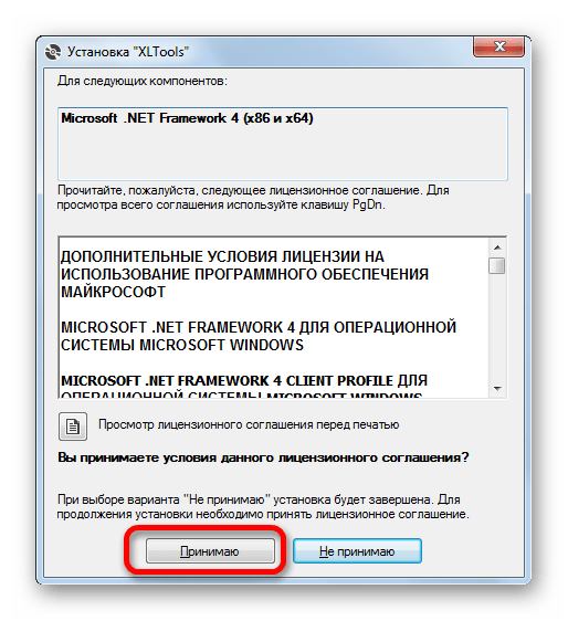
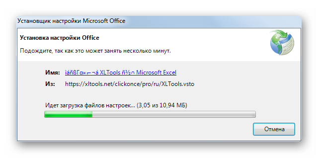
- После того, как вы скачали файл надстройки xltools.exe, следует приступить к его установке. Для запуска инсталлятора нужно произвести двойной щелчок левой кнопки мыши по установочному файлу. После этого запустится окно, в котором нужно будет подтвердить согласие с лицензионным соглашением на использование продукции компании Microsoft — NET Framework 4. Для этого всего лишь нужно кликнуть по кнопке «Принимаю» внизу окошка.
- После этого установщик производит загрузку обязательных файлов и начинает процесс их установки.
- Далее откроется окно, в котором вы должны подтвердить свое согласие на установку этой надстройки. Для этого нужно щелкнуть по кнопке «Установить».
- Затем начинается процедура установки непосредственно самой надстройки.
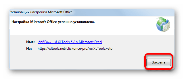
- После её завершения откроется окно, в котором будет сообщаться, что инсталляция успешно выполнена. В указанном окне достаточно нажать на кнопку «Закрыть».
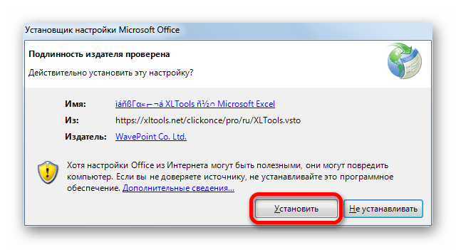
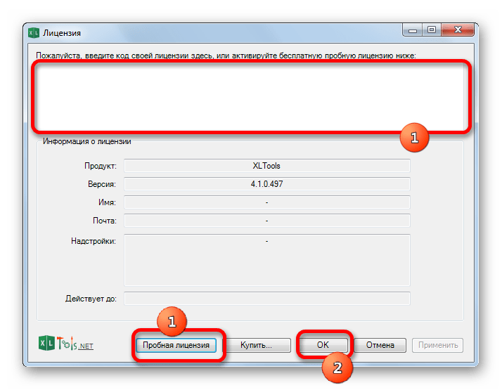
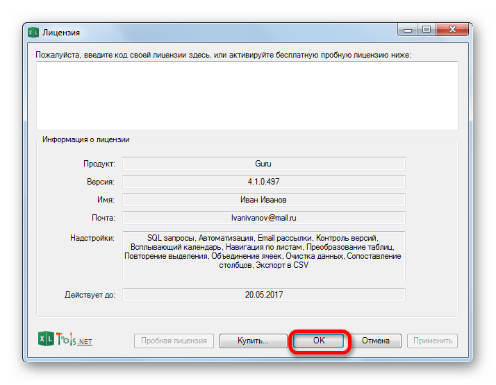
- Надстройка установлена и теперь можно запускать файл Excel, в котором нужно организовать SQL запрос. Вместе с листом Эксель открывается окно для ввода кода лицензии XLTools. Если у вас имеется код, то нужно ввести его в соответствующее поле и нажать на кнопку «OK». Если вы желаете использовать бесплатную версию на 14 дней, то следует просто нажать на кнопку «Пробная лицензия».
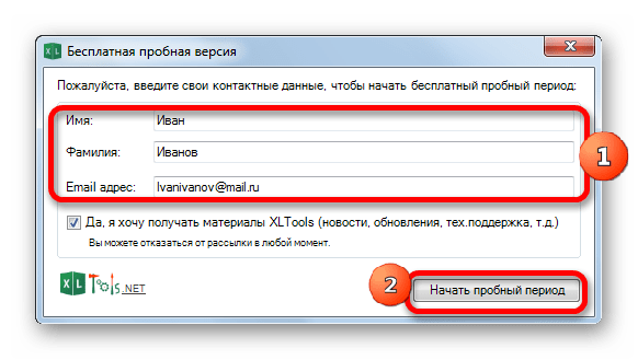
- При выборе пробной лицензии открывается ещё одно небольшое окошко, где нужно указать своё имя и фамилию (можно псевдоним) и электронную почту. После этого жмите на кнопку «Начать пробный период».
- Далее мы возвращаемся к окну лицензии. Как видим, введенные вами значения уже отображаются. Теперь нужно просто нажать на кнопку «OK».
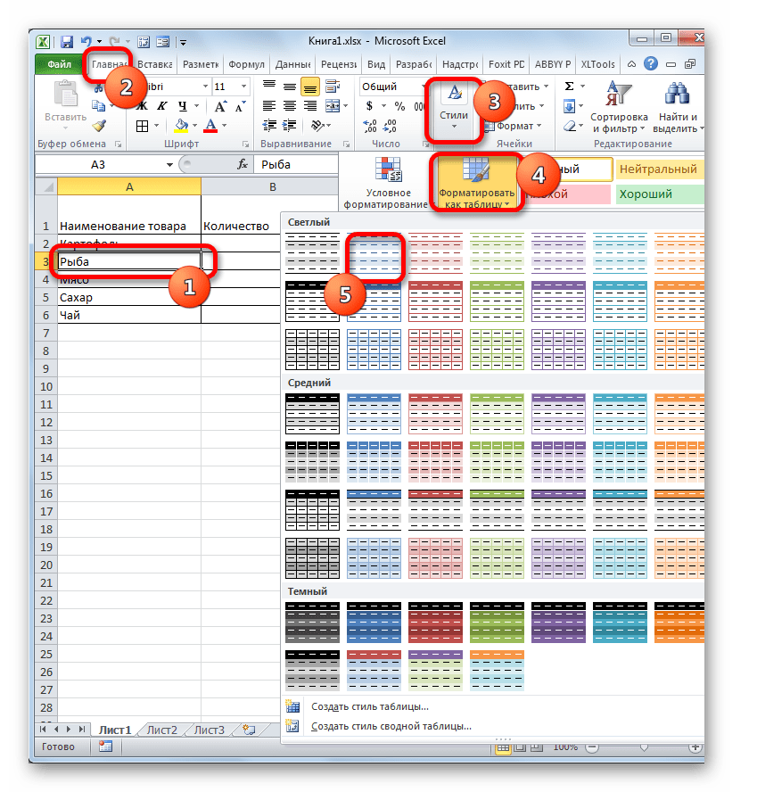
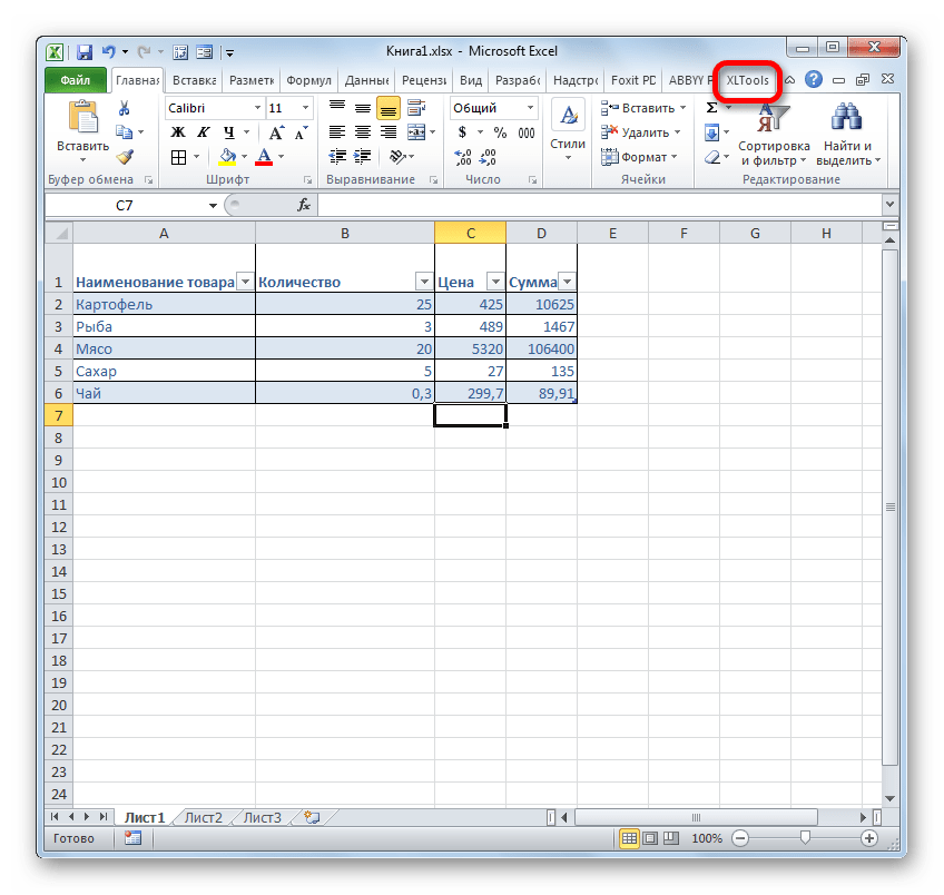
- После того, как вы проделаете вышеуказанные манипуляции, в вашем экземпляре Эксель появится новая вкладка – «XLTools». Но не спешим переходить в неё. Прежде, чем создавать запрос, нужно преобразовать табличный массив, с которым мы будем работать, в так называемую, «умную» таблицу и присвоить ей имя.
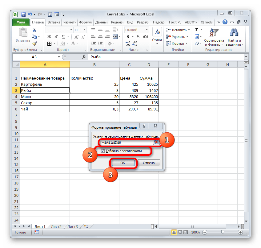
Для этого выделяем указанный массив или любой его элемент. Находясь во вкладке «Главная» щелкаем по значку «Форматировать как таблицу». Он размещен на ленте в блоке инструментов «Стили». После этого открывается список выбора различных стилей. Выбираем тот стиль, который вы считаете нужным. На функциональность таблицы указанный выбор никак не повлияет, так что основывайте свой выбор исключительно на основе предпочтений визуального отображения. - Вслед за этим запускается небольшое окошко. В нем указываются координаты таблицы. Как правило, программа сама «подхватывает» полный адрес массива, даже если вы выделили только одну ячейку в нем. Но на всякий случай не мешает проверить ту информацию, которая находится в поле «Укажите расположение данных таблицы». Также нужно обратить внимание, чтобы около пункта «Таблица с заголовками», стояла галочка, если заголовки в вашем массиве действительно присутствуют. Затем жмите на кнопку «OK».
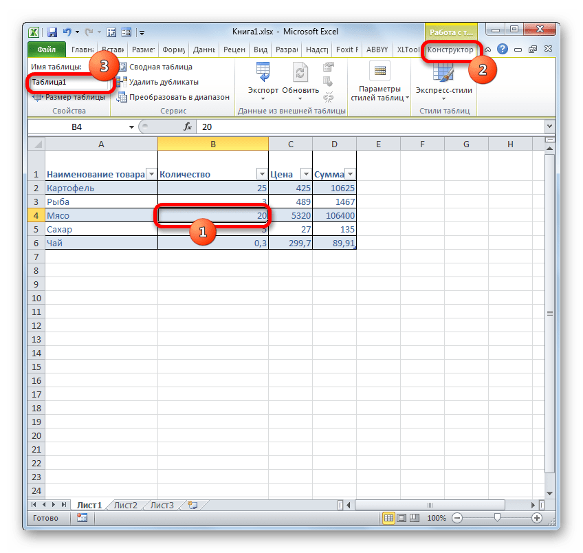
- После этого весь указанный диапазон будет отформатирован, как таблица, что повлияет как на его свойства (например, растягивание), так и на визуальное отображение. Указанной таблице будет присвоено имя. Чтобы его узнать и по желанию изменить, клацаем по любому элементу массива. На ленте появляется дополнительная группа вкладок – «Работа с таблицами». Перемещаемся во вкладку «Конструктор», размещенную в ней. На ленте в блоке инструментов «Свойства» в поле «Имя таблицы» будет указано наименование массива, которое ему присвоила программа автоматически.
- При желании это наименование пользователь может изменить на более информативное, просто вписав в поле с клавиатуры желаемый вариант и нажав на клавишу Enter.
- После этого таблица готова и можно переходить непосредственно к организации запроса. Перемещаемся во вкладку «XLTools».
- После перехода на ленте в блоке инструментов «SQL запросы» щелкаем по значку «Выполнить SQL».
- Запускается окно выполнения SQL запроса. В левой его области следует указать лист документа и таблицу на древе данных, к которой будет формироваться запрос.
В правой области окна, которая занимает его большую часть, располагается сам редактор SQL запросов. В нем нужно писать программный код. Наименования столбцов выбранной таблицы там уже будут отображаться автоматически. Выбор столбцов для обработки производится с помощью команды SELECT. Нужно оставить в перечне только те колонки, которые вы желаете, чтобы указанная команда обрабатывала.
Далее пишется текст команды, которую вы хотите применить к выбранным объектам. Команды составляются при помощи специальных операторов. Вот основные операторы SQL:
- ORDER BY – сортировка значений;
- JOIN – объединение таблиц;
- GROUP BY – группировка значений;
- SUM – суммирование значений;
- DISTINCT – удаление дубликатов.
Кроме того, в построении запроса можно использовать операторы MAX, MIN, AVG, COUNT, LEFT и др.
В нижней части окна следует указать, куда именно будет выводиться результат обработки. Это может быть новый лист книги (по умолчанию) или определенный диапазон на текущем листе. В последнем случае нужно переставить переключатель в соответствующую позицию и указать координаты этого диапазона.
После того, как запрос составлен и соответствующие настройки произведены, жмем на кнопку «Выполнить» в нижней части окна. После этого введенная операция будет произведена.


Урок: «Умные» таблицы в Экселе
Способ 2: использование встроенных инструментов Excel
Существует также способ создать SQL запрос к выбранному источнику данных с помощью встроенных инструментов Эксель.
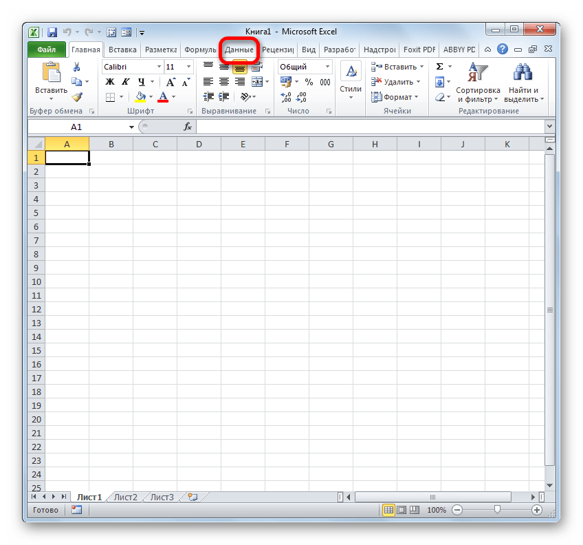
- Запускаем программу Excel. После этого перемещаемся во вкладку «Данные».
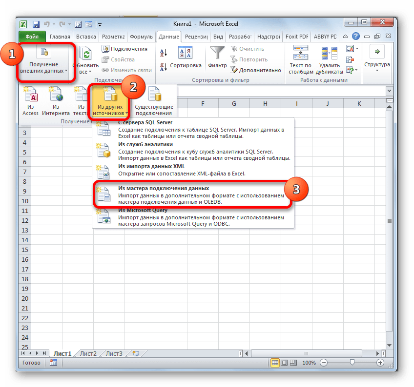
- В блоке инструментов «Получение внешних данных», который расположен на ленте, жмем на значок «Из других источников». Открывается список дальнейших вариантов действий. Выбираем в нем пункт «Из мастера подключения данных».
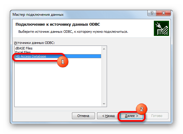
- Запускается Мастер подключения данных. В перечне типов источников данных выбираем «ODBC DSN». После этого щелкаем по кнопке «Далее».
- Открывается окно Мастера подключения данных, в котором нужно выбрать тип источника. Выбираем наименование «MS Access Database». Затем щелкаем по кнопке «Далее».
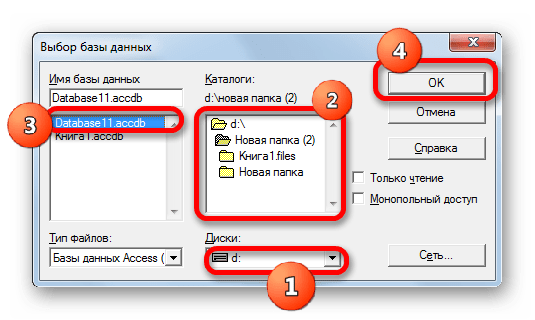
- Открывается небольшое окошко навигации, в котором следует перейти в директорию расположения базы данных в формате mdb или accdb и выбрать нужный файл БД. Навигация между логическими дисками при этом производится в специальном поле «Диски». Между каталогами производится переход в центральной области окна под названием «Каталоги». В левой области окна отображаются файлы, расположенные в текущем каталоге, если они имеют расширение mdb или accdb. Именно в этой области нужно выбрать наименование файла, после чего кликнуть на кнопку «OK».
- Вслед за этим запускается окно выбора таблицы в указанной базе данных. В центральной области следует выбрать наименование нужной таблицы (если их несколько), а потом нажать на кнопку «Далее».
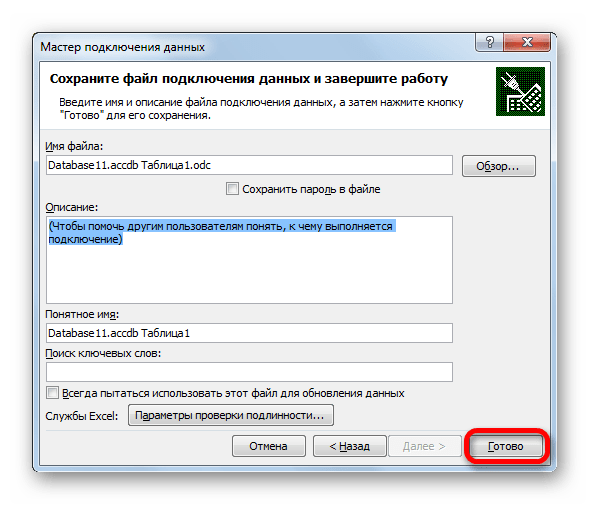
- После этого открывается окно сохранения файла подключения данных. Тут указаны основные сведения о подключении, которое мы настроили. В данном окне достаточно нажать на кнопку «Готово».
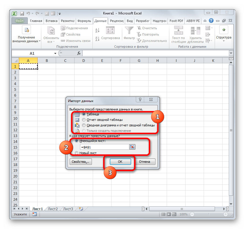
- На листе Excel запускается окошко импорта данных. В нем можно указать, в каком именно виде вы хотите, чтобы данные были представлены:
- Таблица;
- Отчёт сводной таблицы;
- Сводная диаграмма.
Выбираем нужный вариант. Чуть ниже требуется указать, куда именно следует поместить данные: на новый лист или на текущем листе. В последнем случае предоставляется также возможность выбора координат размещения. По умолчанию данные размещаются на текущем листе. Левый верхний угол импортируемого объекта размещается в ячейке A1.
После того, как все настройки импорта указаны, жмем на кнопку «OK».
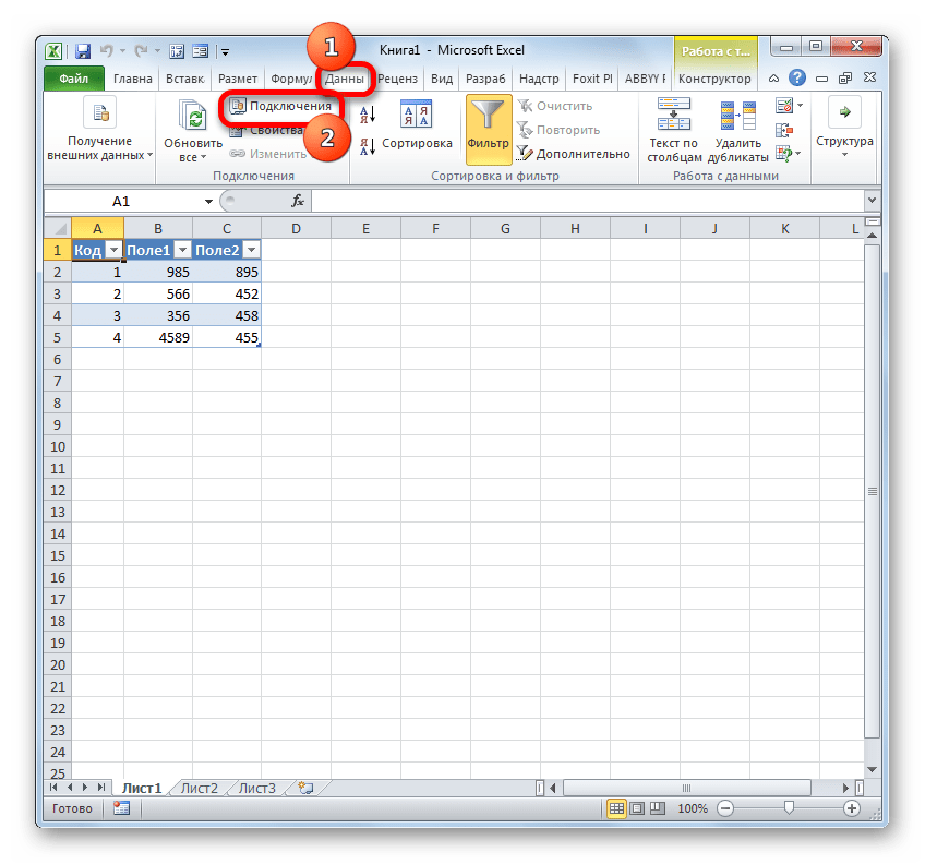
- Как видим, таблица из базы данных перемещена на лист. Затем перемещаемся во вкладку «Данные» и щелкаем по кнопке «Подключения», которая размещена на ленте в блоке инструментов с одноименным названием.
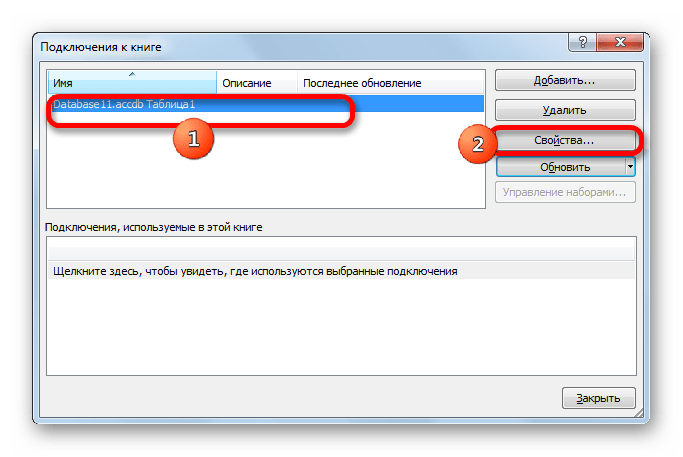
- После этого запускается окно подключения к книге. В нем мы видим наименование ранее подключенной нами базы данных. Если подключенных БД несколько, то выбираем нужную и выделяем её. После этого щелкаем по кнопке «Свойства…» в правой части окна.
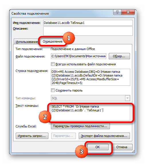
- Запускается окно свойств подключения. Перемещаемся в нем во вкладку «Определение». В поле «Текст команды», находящееся внизу текущего окна, записываем SQL команду в соответствии с синтаксисом данного языка, о котором мы вкратце говорили при рассмотрении Способа 1. Затем жмем на кнопку «OK».
- После этого производится автоматический возврат к окну подключения к книге. Нам остается только кликнуть по кнопке «Обновить» в нем. Происходит обращение к базе данных с запросом, после чего БД возвращает результаты его обработки назад на лист Excel, в ранее перенесенную нами таблицу.


Способ 3: подключение к серверу SQL Server
Кроме того, посредством инструментов Excel существует возможность соединения с сервером SQL Server и посыла к нему запросов. Построение запроса не отличается от предыдущего варианта, но прежде всего, нужно установить само подключение. Посмотрим, как это сделать.
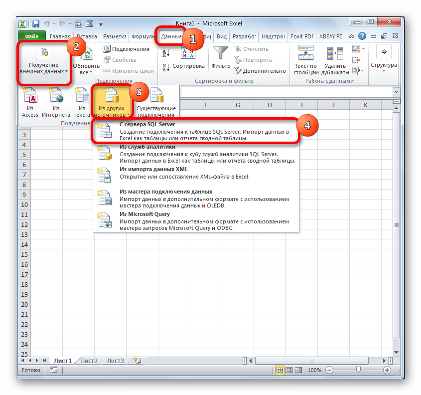
- Запускаем программу Excel и переходим во вкладку «Данные». После этого щелкаем по кнопке «Из других источников», которая размещается на ленте в блоке инструментов «Получение внешних данных». На этот раз из раскрывшегося списка выбираем вариант «С сервера SQL Server».
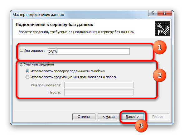
- Происходит открытие окна подключения к серверу баз данных. В поле «Имя сервера» указываем наименование того сервера, к которому выполняем подключение. В группе параметров «Учетные сведения» нужно определиться, как именно будет происходить подключение: с использованием проверки подлинности Windows или путем введения имени пользователя и пароля. Выставляем переключатель согласно принятому решению. Если вы выбрали второй вариант, то кроме того в соответствующие поля придется ввести имя пользователя и пароль. После того, как все настройки проведены, жмем на кнопку «Далее». После выполнения этого действия происходит подключение к указанному серверу. Дальнейшие действия по организации запроса к базе данных аналогичны тем, которые мы описывали в предыдущем способе.
Как видим, в Экселе SQL запрос можно организовать, как встроенными инструментами программы, так и при помощи сторонних надстроек. Каждый пользователь может выбрать тот вариант, который удобнее для него и является более подходящим для решения конкретно поставленной задачи. Хотя, возможности надстройки XLTools, в целом, все-таки несколько более продвинутые, чем у встроенных инструментов Excel. Главный же недостаток XLTools заключается в том, что срок бесплатного пользования надстройкой ограничен всего двумя календарными неделями.
Еще статьи по данной теме:
Помогла ли Вам статья?
Excel is a combination of rows and columns, and these rows and columns store our data, which in other terms are named records. As Excel is the most common tool, we reserve the data in Excel, making it a database. Therefore, when we put data in Excel in some form of tables in rows and columns and give the table a name, that is a database in Excel. We can also import data from other sources in Excel, given the data format is proper with the Excel format.
For example, you may create a company’s sales report of different regions on a database in Excel for easy access and complete control over data management while working with the program.
Creating an Excel Database
Having the data in Excel will make life easier for you because Excel is a powerful tool where we can play with the data. If you maintain the data in other sources, you may not correctly get all the formulas, dates, and time format. I hope you have experienced this in your daily work. Having the data in the right database platform is very important. Having the data in Excel has its pros and cons. However, if you are a regular user of Excel, it is much easier to work with Excel. This article will show you how to create a database in Excel.
Table of contents
- Creating an Excel Database
- How to Create a Database in Excel?
- Things to Remember While Creating a Database in Excel
- Recommended Articles
You are free to use this image on your website, templates, etc, Please provide us with an attribution linkArticle Link to be Hyperlinked
For eg:
Source: Database in Excel (wallstreetmojo.com)
How to Create a Database in Excel?
We do not see any of the schools are colleges teaching us to Excel as the software in our academics. Whatever business models, we learn a theory until joining the corporate company.
The biggest problem with this theoretical knowledge is it does not support real-time life examples. But, nothing to worry about; we will guide you through the process of creating a database in Excel.
We need to design the Excel worksheet carefully to have accurate data in the database format.
You can download this Create Database Excel Template here – Create Database Excel Template
Follow the below steps to create a database in Excel.
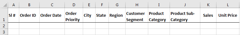
- We must first ensure all the required columns and name each heading properly.

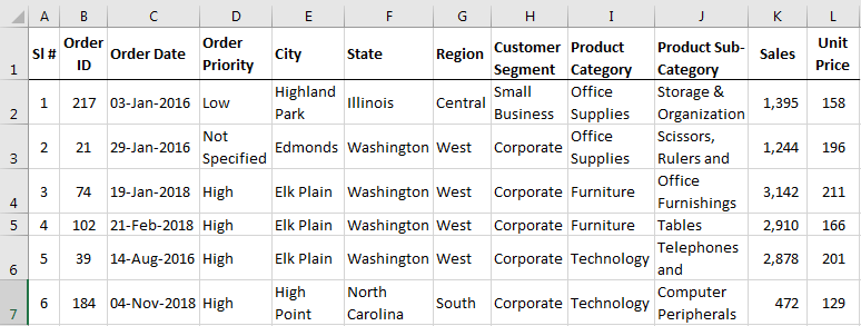
- Once the headers of the data table are clear, we can easily start entering the data just below the respective column headings.

In database terminology, rows are called Records, and columns are called Fields.
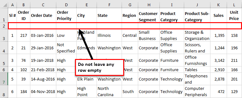
- We cannot leave a single row empty when entering the data. For example, we have entered the headings in the first row, and if we start entering the data from the third row by leaving the 2nd row empty, we are gone.

Not only the first or second row, but we also cannot leave any row empty after entering certain data into the database field.
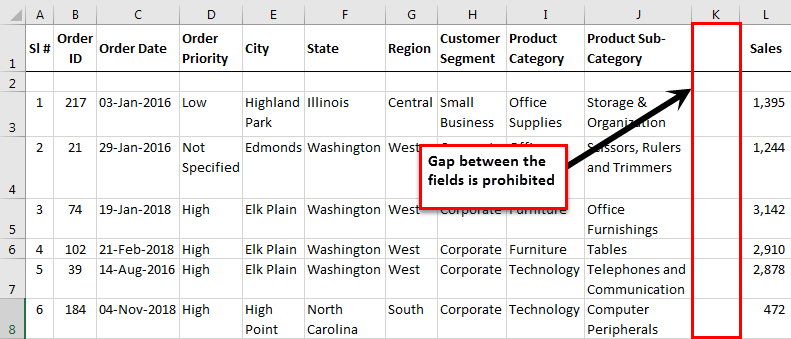
- As we said, each column is called Fields in the database. Similarly, we cannot have an empty field between the data.
We need to enter the fields one after the other. Having a gap of even one column or field is strictly prohibited.

I am so stressed about not having an empty record or field because when the data needs to be exported to other software or the web, as soon as the software sees the blank record or field, it assumes that it is the end of the data. Therefore, it may not consider the full data.
- We must fill in all the data carefully.
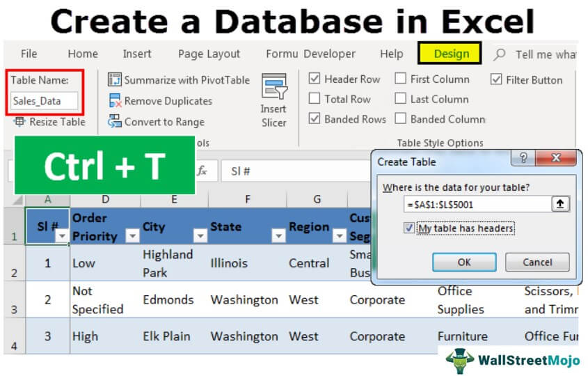
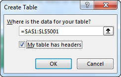
In the above image, I have data all the way from row 1 to row 5001. - The final thing we need to do is convert this data to an excel table. By selecting the data, press Ctrl + T.

- Here, we need to make sure the My table has a header checkbox is ticked and the range is selected properly.

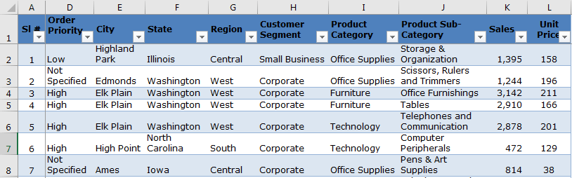
- Then, we must click on OK to complete the table creation. As a result, we may have a table like this now.

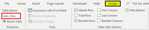
- We must now give a proper name to the table under the table Design tab.

- Since we have created a table, automatically, it would expand whenever we enter the data after the last column.
We have the database ready now. Follow the pros and cons below to have a good hand on your database.

Things to Remember While Creating a Database in Excel
- We can upload the file to MS Access to have a secure database and back up a platform.
- Since we have all the data in Excel, it is very easy for your calculations and statistics.
- Excel is the best tool for database analysis.
- Easy to read and not complicated because of clear fields and records.
- We can filter out the records by using auto filters.
- If possible, sort the data according to date-wise.
- As the data keeps growing, Excel will slow down considerably.
- We cannot share more than 34 MB files with others in an email.
- We can Apply the Pivot tableA Pivot Table is an Excel tool that allows you to extract data in a preferred format (dashboard/reports) from large data sets contained within a worksheet. It can summarize, sort, group, and reorganize data, as well as execute other complex calculations on it.read more and give a detailed analysis of the database.
- We can download the workbook and use it for your practice purpose.
Recommended Articles
This article is a guide to Databases in Excel. Here, we discuss creating a database in Excel with examples and downloadable Excel templates. You may also look at these useful functions in Excel: –
- Excel Database Template
- Match Data using Excel Functions
- Forms for Data Entry in Excel
- Create a Data Table in Excel
- SUMIFS with Dates
Steps to create a database in Excel
- Create a data spreadsheet
- Add or import data
- Convert your data into a table
- Customize the table design and assign a name
- Interact with the data
Every business has numbers to crunch, but not every CEO is a math wiz. That’s why small business owners often outsource their accounting or let their bookkeeper deal with it.
However, there are many other ways you can process data to make operations more efficient. Plus, you probably want to avoid constantly running to someone else for help.
That’s where a basic knowledge of Excel databases comes in handy.
Excel is one of those tools that almost everyone has on their desktop, and you can enjoy its benefits without being a numbers wizard.
Excel databases provide a simple way to analyze data (such as sales numbers and forecasts), look at various calculations, and compare different data sets. Of course, there are advanced formulas and functions if you dive deeper and invest time in becoming a pro. But for many business owners, just knowing how to create a database in Excel will give them a lot of power.
Let’s take a step-by-step tour of using Excel to create a database.
Just so you know
Learn how to make the most of your data with Jotform’s detailed Microsoft Excel tutorial. You can even integrate Jotform with Excel to sync form data to your spreadsheets!
1. Create a data spreadsheet
Start by opening a new Excel sheet.
The Excel sheet is made up of vertical columns and horizontal rows, with each row representing a different line of data. Columns are labeled with letters, and rows are labeled with numbers.
The first row should display the names for each column. Click on a cell in the first row and begin typing to insert header names. The Tab button is a quick way to navigate the table; each time you press the Tab button, you’ll jump to the next column in a row. When you reach the end of a row, the cursor will jump to the first column of the next row, and so on.
2. Add or import data
You can add data in two ways: by entering it manually or importing data from other files, such as text or CSV files.
To add data manually, click on a cell and begin typing. To insert a new row or column, go to the Home tab and look for the Cells section. There you’ll find the Insert dropdown arrow. By clicking on the arrow, you can select the item you want to insert (i.e., column, row, etc.).
To import data from outside sources, click on the Data tab, go to the Get/Transform Data section, and select the source destination. In order to import data successfully, you must ensure that the data has the correct formatting, and formatting depends on the type of source file.
3. Convert your data into a table
To get the functionality of a database, you must convert the data into a table.
Click your mouse on any cell of the data you entered, and then click on Insert >Table. A popup box will appear, showing you the data fields to be included in the table. The table will automatically incorporate all the rows and columns in the block. It’s important not to leave any blank rows in your data block — these act as “breaks” and indicate to the software that they aren’t part of the table.
If the correct fields are shown in the dialog box and your headers are in order, click OK.
Remember, any blank rows are not automatically integrated into the table. To include newly entered data in the table, hover on the small triangle nestled in the bottom right corner of the current table and drag the table border down to include the new data rows.
4. Customize the table design and assign a name
There are several options for table design, but don’t spend a lot of time on this. Making your table easily viewable is the aim of the game.
Click the Design tab on the main menu. Change the table colors with a quick click on one of the predefined color themes. The default table design features banded rows, meaning every second row has a background fill. Many users like this style, as it makes the data easier to view. Uncheck the Banded Rows box if you prefer a clean, white table.
In the far left section of the Design toolbar, you can change the table name. Give it a name that is specific and easy to identify. This will help later down the road when you’re working with many Excel databases.
5. Interact with the data
Once your table is set up, it’s time to start interacting with it and getting the insights you need. Several formulas are predefined in Excel software, including Average, Count, and Sum, among others.
Click on the cell at the base of any data column you want to work with. The cell displays a clickable arrow that opens a dropdown menu of available formulas. Select the formula, and the calculation will automatically appear in the cell.
In the example below, we’re calculating the average number of units sold. The Average formula is an option in the dropdown menu.
The average number of units sold is calculated and appears in the cell.
There are so many ways you can use Excel to perform calculations and derive useful data for decision-making. Now that you’ve created a database in Excel, you can explore all the available features and functionality.
Go beyond Excel: Working with Jotform Tables
While Excel is a longstanding favorite for number crunching, tools like Jotform Tables can give you much more than a spreadsheet. Jotform Tables provides a full workspace for managing, tracking, and processing data, and integrating it into workflows and collaboration for smoother operations.
If you work with Excel databases, you can easily import them into Jotform Tables and continue your data management there. And as a free tool, Jotform Tables requires none of the investment and licenses you need with Excel.
For companies already using Jotform, Jotform Tables is the next step, as it enables you to build effective data-based strategies so your business can truly excel.
This article is originally published on Nov 10, 2020, and updated on Feb 24, 2023.