
A range is a group or block of cells in a worksheet that are selected or highlighted. Also, a range can be a group or block of cell references that are entered as an argument for a function, used to create a graph, or used to bookmark data.
The information in this article applies to Excel versions 2019, 2016, 2013, 2010, Excel Online, and Excel for Mac.
Contiguous and Non-Contiguous Ranges
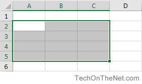
A contiguous range of cells is a group of highlighted cells that are adjacent to each other, such as the range C1 to C5 shown in the image above.
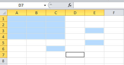
A non-contiguous range consists of two or more separate blocks of cells. These blocks can be separated by rows or columns as shown by the ranges A1 to A5 and C1 to C5.
Both contiguous and non-contiguous ranges can include hundreds or even thousands of cells and span worksheets and workbooks.
Range Names
Ranges are so important in Excel and Google Spreadsheets that names can be given to specific ranges to make them easier to work with and reuse when referencing them in charts and formulas.
Select a Range in a Worksheet
When cells have been selected, they are surrounded by an outline or border. By default, this outline or border surrounds only one cell in a worksheet at a time, which is known as the active cell. Changes to a worksheet, such as data editing or formatting, affect the active cell.
When a range of more than one cell is selected, changes to the worksheet, with certain exceptions such as data entry and editing, affect all cells in the selected range.
There a number of ways to select a range in a worksheet. These include using the mouse, the keyboard, the name box, or a combination of the three.
To create a range consisting of adjacent cells, drag with the mouse or use a combination of the Shift and four arrow keys on the keyboard. To create ranges consisting of non-adjacent cells, use the mouse and keyboard or just the keyboard.
Select a Range for Use in a Formula or Chart
When entering a range of cell references as an argument for a function or when creating a chart, in addition to typing in the range manually, the range can also be selected using pointing.
Ranges are identified by the cell references or addresses of the cells in the upper left and lower right corners of the range. These two references are separated by a colon. The colon tells Excel to include all the cells between these start and endpoints.
Range vs. Array
At times the terms range and array seem to be used interchangeably for Excel and Google Sheets since both terms are related to the use of multiple cells in a workbook or file.
To be precise, the difference is because a range refers to the selection or identification of multiple cells (such as A1:A5) and an array refers to the values located in those cells (such as {1;2;5;4;3}).
Some functions, such as SUMPRODUCT and INDEX, take arrays as arguments. Other functions, such as SUMIF and COUNTIF, accept only ranges for arguments.
That’s not to say that a range of cell references cannot be entered as arguments for SUMPRODUCT and INDEX. These functions extract the values from the range and translate them into an array.
For example, the following formulas both return a result of 69 as shown in cells E1 and E2 in the image.
=SUMPRODUCT(A1:A5,C1:C5)
=SUMPRODUCT({1;2;5;4;3},{1;4;8;2;4})
On the other hand, SUMIF and COUNTIF do not accept arrays as arguments. So, while the formula below returns an answer of 3 (see cell E3 in the image), the same formula with an array would not be accepted.
COUNTIF(A1:A5,"<4")
As a result, the program displays a message box listing possible problems and corrections.
Thanks for letting us know!
Get the Latest Tech News Delivered Every Day
Subscribe
Find Range in Excel (Table of Contents)
- Range in Excel
- How to Find Range in Excel?
Range in Excel
Whenever we talk about the range in excel, it can be one cell or can be a collection of cells. It can be the adjacent cells or non-adjacent cells in the dataset.
What is Range in Excel & its Formula?
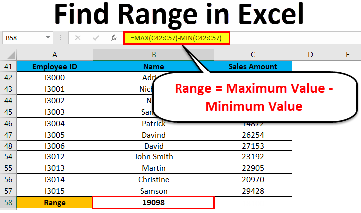
A range is the collection of values spread between the Maximum value and the Minimum value. A range is a difference between the Largest (maximum) value and the Shortest (minimum) value in a given dataset in mathematical terms.
Range defines the spread of values in any dataset. It calculates by a simple formula like below:
Range = Maximum Value – Minimum Value
How to Find Range in Excel?
Finding a range is a very simple process, and it is calculated using the Excel in-built functions MAX and MIN. Let’s understand the working of finding a range in excel with some examples.
You can download this Find Range Excel Template here – Find Range Excel Template
Range in Excel – Example #1
We have given below a list of values:
23, 11, 45, 21, 2, 60, 10, 35
The largest number in the above-given range is 60, and the smallest number is 2.
Thus, the Range = 60-2 = 58
Explanation:
- In this above example, the Range is 58 in the given dataset, which defines the span of the dataset. It gave you a visual indication of the range as we are looking for the highest and smallest point.
- If the dataset is large, it gives you the widespread of the result.
- If the dataset is small, it gives you a closely centered result.
A process of defining the range in Excel
For defining the range, we need to find out the maximum and minimum values of the dataset. In this process, two function plays a very important role. They are:
- MAX
- MIN
Use of MAX function:
Let’s take an example to understand the usage of this function.
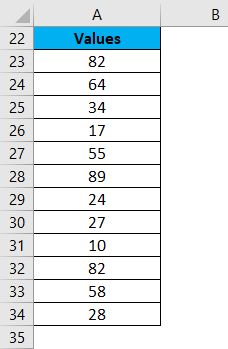
Range in Excel – Example #2
We have given some set of values:
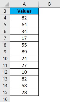
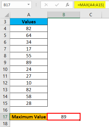
For finding the maximum value from the dataset, we will apply here the MAX function as below screenshot:
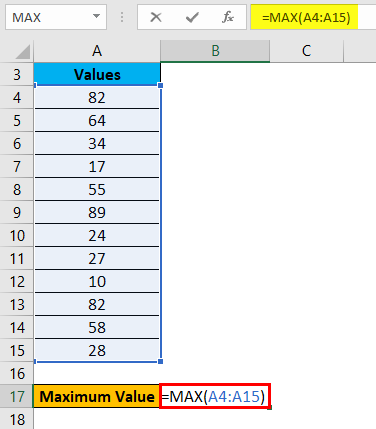
Hit enter, and it will give you the maximum value. The result is shown below:
Range in Excel – Example #3
Use of MIN function:
Let’s take the same above dataset to understand the usage of this function.
For calculating the minimum value from the given dataset, we will apply the MIN function here as per the below screenshot.
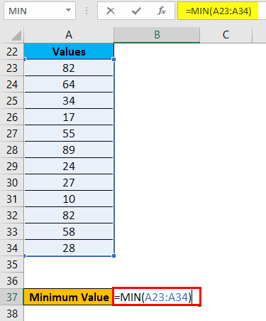
Press ENTER key, and it will give you the minimum value. The result is given below:
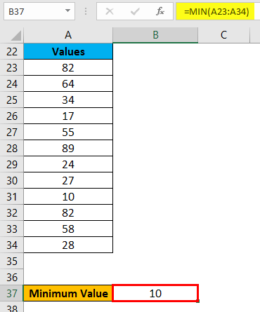
Now you can find out the range of the dataset after taking the difference between Maximum and Minimum value.
We can reduce the steps for calculating the range of a dataset by using the MAX and MIN functions together in one line.
For this, we again take an example to understand the process.
Range in Excel – Example #4
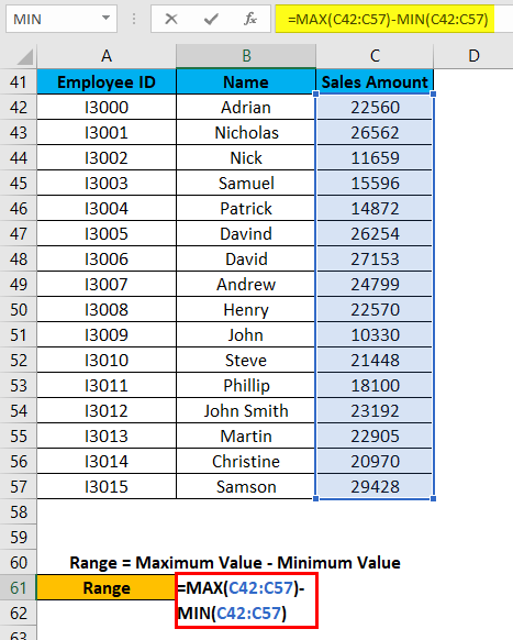
Let’s assume the below dataset of a company employee with their achieved sales target.
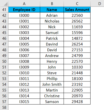
Now for identifying the span of sales amount in the above dataset, we will calculate the range. For this, we will follow the same procedure as we did in the above examples.
We will apply the MAX and MIN functions for calculating the Maximum and Minimum sales amount in the data.
For finding the range of sales amount, we will apply the below formula:
Range = Maximum Value – Minimum Value
Refer to the below screenshot:
Press Enter key, and it will give you the range of the dataset. The result is shown below:
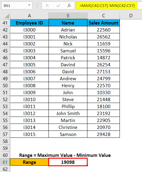
As we can see in the above screenshot, we applied the MAX and MIN formulas in one line, and by calculating their results difference, we found the range of the dataset.
Things to Remember
- If the values are available in the non-adjacent cells, you want to find out the range; you can pass the cell address individually, separated with a comma as an argument of the MAX and MIN functions.
- We can reduce the steps for calculating the range by applying MAX and MIN functions in one line. (Refer to Example 4 for your reference)
Recommended Articles
This has been a guide to Range in Excel. Here we discuss how to find Range in Excel along with excel examples and downloadable excel template. You may learn more about Excel from the following articles –
- Excel Function for Range
- Excel Named Range
- VBA Range
- VBA Selecting Range
Содержание
- Объект Range (Excel)
- Примечания
- Пример
- Методы
- Свойства
- См. также
- Поддержка и обратная связь
- Cell Range In Excel With Operations and Examples
- What is Cell Range in Excel
- Select Single Cell Range in Excel
- Regular Multiple Range Selection
- Irregular Multiple Range Selection
- Column Range Selection Using Mouse and Keyboard
- Row Cell Range Selection with Mouse and Keyboard
- Get Range Selection for A Function of Excel
- How to Autofill Numbers for the Selected Cell Range in Excel
- Copy Same Number to Certain Cell Range
- Autofill Number in Multiples of 2 to Certain Cell Range
- Autofill Dates in the Certain Cell Range in Excel
- Generate Sequence of Months in Cell Range in Excel
Объект Range (Excel)
Представляет ячейку, строку, столбец или группу ячеек, содержащую один или несколько смежных блоков ячеек или объемный диапазон.
Хотите создавать решения, которые расширяют возможности Office на разнообразных платформах? Ознакомьтесь с новой моделью надстроек Office. Надстройки Office занимают меньше места по сравнению с надстройками и решениями VSTO, и вы можете создавать их, используя практически любую технологию веб-программирования, например HTML5, JavaScript, CSS3 и XML.
Примечания
Элемент по умолчанию объекта Range направляет вызовы без параметров в свойство Value, а вызовы с параметрами — в элемент Item. Таким образом, someRange = someOtherRange соответствует someRange.Value = someOtherRange.Value , someRange(1) соответствует someRange.Item(1) и someRange(1,1) соответствует someRange.Item(1,1) .
В разделе Пример описаны следующие свойства и методы для возврата объекта Range:
- Свойства Range и Cells объекта Worksheet
- Свойства Range и Cells объекта Range
- Свойства Rows и Columns объекта Worksheet
- Свойства Rows и Columns объекта Range
- Свойство Offset объекта Range
- Метод Union объекта Application
Пример
Чтобы вернуть объект Range, представляющий одну ячейку или диапазон ячеек, используйте синтаксис Range ( arg ), где arg обозначает диапазон. В следующем примере значение ячейки A1 помещается в ячейку A5.
В следующем примере диапазон A1:H8 заполняется случайными числами путем задания формулы для каждой ячейки в диапазоне. При использовании без квалификатора объекта (объекта слева от точки) свойство Range возвращает диапазон на активном листе. Если активное окно не является листом, метод завершается с ошибкой.
Используйте метод Activate объекта Worksheet, чтобы активировать лист перед использованием свойства Range без явного квалификатора объекта.
В следующем примере очищается содержимое диапазона Criteria.
Если используется текстовый аргумент для адреса диапазона, необходимо указать адрес в нотации стиля A1 (нельзя использовать нотацию в стиле R1C1).
Чтобы получить диапазон, содержащий все отдельные ячейки листа, используйте свойство Cells на листе. Вы можете обращаться к отдельным ячейкам, используя синтаксис Item(строка, столбец), где строка — индекс строки, а столбец — индекс столбца. Свойство Item можно пропустить, так как вызов направляется к нему с помощью элемента по умолчанию объекта Range. В следующем примере на первом листе активной книги ячейке A1 присваивается значение 24, а в ячейке B1 — значение 42.
В следующем примере задается формула для ячейки A2.
Хотя также можно использовать Range(«A1») , чтобы вернуть значение ячейки A1, иногда свойство Cells может быть удобнее, так как позволяет использовать переменную для строки или столбца. В следующем примере создаются заголовки столбцов и строк на листе Sheet1. Обратите внимание, что после активации листа можно использовать свойство Cells без явного объявления листа (оно возвращает ячейку на активном листе).
Хотя для изменения ссылок в стиле A1 можно использовать строковые функции Visual Basic, проще (и лучше при программировании) использовать нотацию Cells(1, 1) .
Используйте синтаксис_выражение_.Cells, где выражение возвращает объект Range, чтобы получить диапазон с тем же адресом, состоящий из отдельных ячеек. В таком диапазоне отдельные ячейки доступны с помощью синтаксиса Item(строка, столбец) относительно левого верхнего угла первой области диапазона. Свойство Item можно пропустить, так как вызов направляется к нему с помощью элемента по умолчанию объекта Range. В следующем примере на первом листе активной книги в ячейках C5 и D5 указывается формула.
Чтобы вернуть объект Range, используйте синтаксис Range ( ячейка1, ячейка2 ), где ячейка1 и ячейка2 — это объекты Range, указывающие начальную и конечную ячейки. В следующем примере устанавливается тип линии границы для ячеек A1:J10.
Имейте в виду, что точка перед каждым появлением свойства Cells является обязательной, если результат предыдущего оператора With нужно применять к свойству Cells. В данном случае указано, что ячейки расположены на листе один (без точки свойство Cells будет возвращать ячейки активного листа).
Чтобы получить диапазон, содержащий все строки листа, используйте свойство Rows на листе. Вы можете обращаться к отдельным строкам с помощью синтаксиса Item(строка), где строка — это индекс строки. Свойство Item можно пропустить, так как вызов направляется к нему с помощью элемента по умолчанию объекта Range.
Недопустимо указывать второй параметр свойства Item для диапазонов, состоящих из строк. Сначала нужно преобразовать их в отдельные ячейки, используя свойство Cells.
В следующем примере удаляются строки 5 и 10 первого листа активной книги.
Чтобы получить диапазон, содержащий все столбцы листа, используйте свойство Columns на листе. Вы можете обращаться к отдельным столбцам с помощью синтаксиса Item(строка) [sic], где строка — это индекс столбца в виде числа или адреса столбца в формате А1. Свойство Item можно пропустить, так как вызов направляется к нему с помощью элемента по умолчанию объекта Range.
Недопустимо указывать второй параметр свойства Item для диапазонов, состоящих из столбцов. Сначала нужно преобразовать их в отдельные ячейки, используя свойство Cells.
В следующем примере удаляются столбцы B, C, E и J первого листа активной книги.
Используйте синтаксис_выражение_.Rows, где выражение возвращает объект Range, чтобы получить диапазон, состоящий из строк первой области диапазона. Вы можете обращаться к отдельным строкам с помощью синтаксиса Item(строка), где строка — это относительный индекс строки от верхнего края первой области диапазона. Свойство Item можно пропустить, так как вызов направляется к нему с помощью элемента по умолчанию объекта Range.
Недопустимо указывать второй параметр свойства Item для диапазонов, состоящих из строк. Сначала нужно преобразовать их в отдельные ячейки, используя свойство Cells.
В следующем примере удаляются диапазоны C8:D8 и C6:D6 первого листа активной книги.
Используйте синтаксис_выражение_.Columns, где выражение возвращает объект Range, чтобы получить диапазон, состоящий из столбцов первой области диапазона. Вы можете обращаться к отдельным столбцам с помощью синтаксиса Item(строка) [sic], где строка — это относительный индекс столбца от левого края первой области диапазона, указанный в виде числа или адреса столбца в формате A1. Свойство Item можно пропустить, так как вызов направляется к нему с помощью элемента по умолчанию объекта Range.
Недопустимо указывать второй параметр свойства Item для диапазонов, состоящих из столбцов. Сначала нужно преобразовать их в отдельные ячейки, используя свойство Cells.
В следующем примере удаляются диапазоны L2:L10, G2:G10, F2:F10 и D2:D10 первого листа активной книги.
Чтобы вернуть диапазон с указанным смещением относительно другого диапазона, используйте синтаксис Offset ( строка, столбец ), где строка и столбец — это смещения строк и столбцов. В следующем примере выделяются ячейки, расположенные на три строки вниз и на один столбец вправо от ячейки в левом верхнем углу текущего выделенного фрагмента. Нельзя выбрать ячейку, которая находится не на активном листе, поэтому сначала необходимо активировать лист.
Используйте синтаксис Union ( диапазон1, диапазон2, . ) для возврата диапазонов из нескольких областей, то есть диапазонов, состоящих из двух или более смежных блоков ячеек. В следующем примере создается объект, определенный как объединение диапазонов A1:B2 и C3:D4, а затем выбирается определенный диапазон.
При работе с выделенными фрагментами, содержащими несколько областей, удобно применять свойство Areas. Оно разделяет выделенный фрагмент с несколькими областями на отдельные объекты Range, а затем возвращает объекты в виде коллекции. Используйте свойство Count в возвращенной коллекции, чтобы убедиться, что выделение содержит более одной области, как показано в следующем примере.
В этом примере используется метод AdvancedFilter объекта Range для создания списка уникальных значений, а также количества появлений этих уникальных значений в диапазоне столбца A.
Методы
Свойства
См. также
Поддержка и обратная связь
Есть вопросы или отзывы, касающиеся Office VBA или этой статьи? Руководство по другим способам получения поддержки и отправки отзывов см. в статье Поддержка Office VBA и обратная связь.
Источник
Cell Range In Excel With Operations and Examples
In this tutorial, learn to use Cell Range In Excel with its different operations. A cell range is a collection of two or more cells to use in Excel formula. You can perform operations over single or multiple cells in MS Excel.
Table of Contents
What is Cell Range in Excel
A cell range is a group of cells you select to use in functions and perform certain operations. The cell you have to use for the range is the intersection of rows and columns.
You can select multiple cells in a regular and irregular manner. To use the range in any function of Excel, you have to select the cell range with the method given below. You may also like to read post on rows and columns to create a cell in MS Excel.
Select Single Cell Range in Excel
A single cell is the intersection of the row and column of excel. If you click on any cell of the Excel sheet, you can find that it contains a column name and row name.
Let us take an example for the image given below. The below-selected cell is the intersection of column B and row 3. You can read the cell as the combination of row and column name as B3.
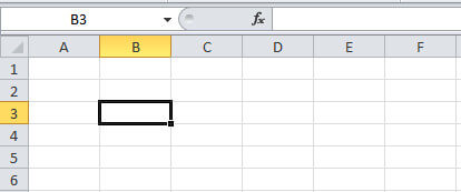
The same rule you have to follow the same naming rule when you select any cell.
Regular Multiple Range Selection
It the method of selecting multiple cells in a certain pattern like square, rectangular, etc. You can select the small and larger area of cells using this method.
To select your pattern, you have followed the steps given below.
Step 1: Go to start cell using mouse or keyboard.
Step 2: Hold ‘shift’ key of the keyboard.
Step 3: Click the last cell
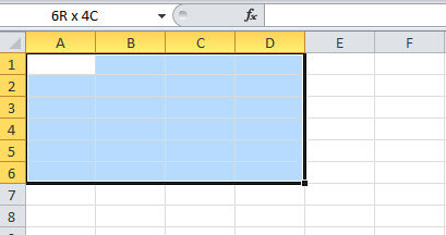
Example: Suppose you want to select the range (A1: D6) as you check in the above image. You have to first go to the cell A1 using your mouse or keyboard. Now, hold the keyboard ‘shift’ key and click the cell D6. This will select the required cell range as given in the above image.
Irregular Multiple Range Selection
An irregular selection is the selection of multiple cells without any patterns. You have to select any numbers of cells in Excel.
To select an irregular pattern, you have to follow the below-given steps:
Step 1: Click on the start cell using the mouse.
Step 2: Hold ‘ctrl’ key of your keyboard.
Step 3: Click the cells you want to select
Example: Suppose you want to select the range (A1:C4,C6,E3,E5) given in the above image. Click the start cell or visit start cell using the arrow key of the keyboard. Now, hold the ‘ctrl’ key and click C4. Again click C6, E3, and E5 cells to select with the hold of the ‘ctrl’ keyboard key.
Column Range Selection Using Mouse and Keyboard
If you select all column cell, this also describes the range in Excel. To select all the cells of a column, you can use either your mouse or keyboard depend upon your choice. below are the methods to select all column cell.
Using Mouse
Step 1: Click the column cell name.
Using Keyboard
Step 1: Go the cell to select the column for.
Step 2: Hold ‘ctrl’ and press ‘space’ key of the keyboard.
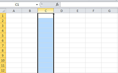
Example Suppose you want to select all the cells of column C given in the above image. You have to just click the column name C using the mouse.
If you want to select using the keyboard, you have to go the column C using arrow key. After that hold the ‘ctrl’ key and press the ‘space’ button of your keyboard. You may also like to read post on how to insert a new column in Excel using a keyboard.
Row Cell Range Selection with Mouse and Keyboard
To select all the cell range of a row, you can use a keyboard or mouse. For mouse use, you have to click the row name given to the left of the cell.
If you want to select all the row cell using only the keyboard, you have to follow the below-given steps.
Step 1: Go to the cell for the row you want using the arrow key.
Step 2: Hold the ‘shift’ key and press ‘space’ button of the keyboard to select the row.
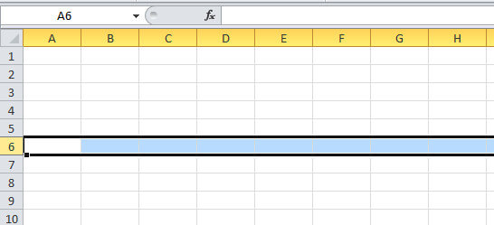
Example: If you want to select the row named 6 as given above. You have to click the name of the row using the mouse. You can also select a row using your keyboard shortcut. Go to any cell of row 6 using your keyboard arrow key. Now, hold the ‘shift’ key and push the ‘space’ bar of your keyboard.`
This will select the row with name 6. You may also like to read post on how to add a new row using MS Excel using the keyboard.
Get Range Selection for A Function of Excel
If you want to select the range from A1 to D7. Go to the cell A1 to start selecting the range. You have to select the range by pressing and holding the keyboard shift key. Now, click the cell D7 to complete the selection.
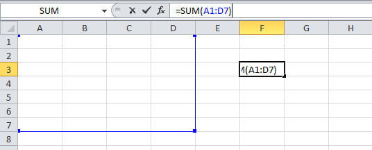
The range after selection showing in the function as SUM(A1:D7). See the image below showing the selection and the output of the sum function.
How to Autofill Numbers for the Selected Cell Range in Excel
Excel comes with many useful features to fill numbers in range. You can autofill range of number in multiple of 1, 2, 3, etc. You have to just grab the plus symbol creates when hovering over the cell. So, let’s create some useful autofill numbers in Excel.
Copy Same Number to Certain Cell Range
Step 1: Go to any cell( e.g.B2) and press the numeric 1 button.
Step 2: Mouse hovers over as indicated arrow location in the below image and holds the left mouse button. You will get a plus(+) sign in place of boxed mouse arrow sign. 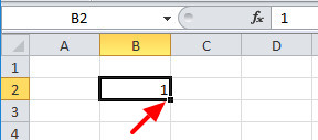
Step 3: Drag the mouse to B7 to get the copy of the number 1 from cell B2 to B7. 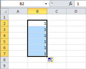
You can copy any number within a certain range using this method.
Autofill Number in Multiples of 2 to Certain Cell Range
Step 1: Go to cell B2, B3 and fill number by pressing button 2,4. In such a manner that 2 is in B2 and 4 is in B3. 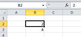
Step 2: Go to cell B2 and press and hold ‘shift’ key. Now, click the B3 cell while holding the ‘shift’ key. This selects the cell B2 and B3. 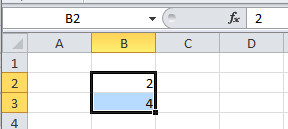
Step 3: Mouse hovers the indicated arrow location given below and holds the left button of the mouse. A plus(+) sign starts to appear in place of boxed mouse arrow sign. 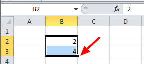
Step 4: Now, you have to just drag the mouse to B8 to get the multiples of 2 from B2 to B8. 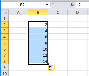
You can fill multiples of any number using the above method. All you have to do is to put the number in multiple first in step 1.
Autofill Dates in the Certain Cell Range in Excel
Step 1: Go to cell B2 and type 1-Aug-95.
Step 2: After typing date, hover over the indicated place given in the image and hold the mouse left button. plus(+) sign showing when you hover over the indicated place. 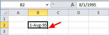
Step 3: Drag the mouse to B11 while holding the mouse left button. This will autofill the date range to a certain cell range. 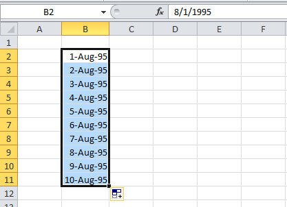
Generate Sequence of Months in Cell Range in Excel
In addition to the above date format, you can also autofill the months. To perform this task and autofill months, follow the given below step-by-step method.
Step 1: Click the cell B2 and type Feb.
Step 2: Now, take your mouse to indicated place as given in the image and hold the mouse left button. A plus(+) sign displays when hovering over the indicated place. 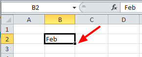
Step 3: You have to just drag the mouse down to the cell B11 with mouse left the button on hold. The selected cell range auto-filled with the sequence of months. 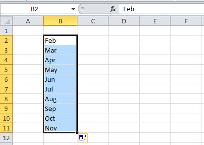
Hope, you like this post of cell range in excel with certain operations. If you have any query regarding the tutorial, please comment below.
Also tell me, what other operations you perform with the range in Excel
Источник

In Microsoft Excel, a range is a collection of cells. A range can be 2 or more cells and those cells don’t necessarily have to be adjacent to each other. Let’s look at some examples to quickly demonstrate the different types of ranges.
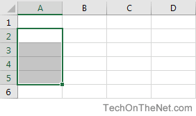
Vertical Range
This vertical range is A2:A5. In this example, if you had selected the entire column A, the range would be A:A.
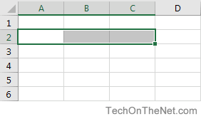
Horizontal Range
This horizontal range is A2:C2. In this example, if you selected the entire row 2, the range would have be 2:2.
Mixed Range
This mixed range is A2:C5. This is a collection of cells that can be from multiple rows and columns.
Multiple Selection Range
This multiple selection range is A2:A3,B4:B5. This is a collection of cells that does not have to be adjacent.
Each range has its own set of coordinates or position in the worksheet such as A2:A5, A2:C2, A2:C5, and so on.
There are many things that you can do with ranges in Excel such as copying, moving, formatting, and naming ranges. Here is a list of topics that explain how to use ranges in Excel.
Cell, Row, Column | Range Examples | Fill a Range | Move a Range | Copy/Paste a Range | Insert Row, Column
A range in Excel is a collection of two or more cells. This chapter gives an overview of some very important range operations.
Cell, Row, Column
Let’s start by selecting a cell, row and column.
1. To select cell C3, click on the box at the intersection of column C and row 3.

2. To select column C, click on the column C header.

3. To select row 3, click on the row 3 header.

Range Examples
A range is a collection of two or more cells.
1. To select the range B2:C4, click on cell B2 and drag it to cell C4.

2. To select a range of individual cells, hold down CTRL and click on each cell that you want to include in the range.

Fill a Range
To fill a range, execute the following steps.
1a. Enter the value 2 into cell B2.

1b. Select cell B2, click on the lower right corner of cell B2 and drag it down to cell B8.

Result:

This dragging technique is very important and you will use it very often in Excel. Here’s another example.
2a. Enter the value 2 into cell B2 and the value 4 into cell B3.

2b. Select cell B2 and cell B3, click on the lower right corner of this range and drag it down.

Excel automatically fills the range based on the pattern of the first two values. That’s pretty cool huh!? Here’s another example.
3a. Enter the date 6/13/2016 into cell B2 and the date 6/16/2016 into cell B3.

3b. Select cell B2 and cell B3, click on the lower right corner of this range and drag it down.

Note: visit our page about AutoFill for many more examples.
Move a Range
To move a range, execute the following steps.
1. Select a range and click on the border of the range.

2. Drag the range to its new location.

Copy/Paste a Range
To copy and paste a range, execute the following steps.
1. Select the range, right click, and then click Copy (or press CTRL + c).

2. Select the cell where you want the first cell of the range to appear, right click, and then click Paste under ‘Paste Options:’ (or press CTRL + v).

Insert Row, Column
To insert a row between the values 20 and 40 below, execute the following steps.
1. Select row 3.

2. Right click, and then click Insert.

Result.

The rows below the new row are shifted down. In a similar way, you can insert a column.