Microsoft excel values only - Word и Excel - помощь в работе с программами

I’m quite new to Excel and completely new to this forum.

I have taken the code from the below forum and modified it to my need.

http://pressf1.pcworld.co.nz/showthread.php?90122-Creating-Macro-to-copy-and-paste-data-into-the-next-empty-column.

Sub copyTotals()
    Dim TargetSht As Worksheet, SourceSht As Worksheet, SourceRow As Integer, SourceCells As Range
    Set SourceSht = ThisWorkbook.Sheets("DUN - Jan")
    Set TargetSht = ThisWorkbook.Sheets("DUN Jan - Jan,Feb,Mar,Apr")
    Set SourceCells = SourceSht.Range("L36,N36")
    If TargetSht.Range("C11").Value = "" Then
        SourceRow = 1
    ElseIf TargetSht.Range("C41") <> "" Then
        MsgBox ("The sheet is full, you need to create a new sheet")
    Else
        SourceRow = TargetSht.Range("C41").End(xlUp).Row + 1
    End If

    SourceCells.Copy TargetSht.Cells(SourceRow, 3)
End Sub

The problem is that the values pasted have the formating of the source and i only want to paste the values.

Can someone please help me with this.

Scimonster

32.6k8 gold badges78 silver badges88 bronze badges

asked Jan 3, 2013 at 8:49

Use .Copy together with .PasteSpecial. Instead of:

SourceCells.Copy TargetSht.Cells(2, SourceCol)

Do this:

SourceCells.Copy
TargetSht.Cells(2, SourceCol).PasteSpecial xlPasteValues

answered Jan 3, 2013 at 8:56

DanDan

10.4k21 silver badges49 bronze badges

Using the macro recorder yields this kind of thing. I use it a lot when stuck.

Selection.PasteSpecial Paste:=xlPasteValues, Operation:=xlNone, SkipBlanks _
    :=False, Transpose:=False

answered Jan 3, 2013 at 23:30

You don’t need to copy and paste to do this (at least in Excel 2010 and above, I think). You just set the .Value of the range to equal itself. eg:

rng.Value = rng.Value

Sheet1.Range("A1:A10").Value = Sheet1.Range("A1:A10").Value

since .Value «Returns or sets a Variant value that represents the value of the specified range.»

Note that this just works for values, not formats.

http://msdn.microsoft.com/en-us/library/office/ff195193(v=office.15).aspx

answered Oct 2, 2014 at 8:42

SJCSJC

6526 silver badges14 bronze badges

right click in the cell and select paste special then you can choose values only

edit: for macros its the same principle
use
.PasteSpecial xlPasteValues
like here

Set rng6 = .Range("A3").End(xlDown).Offset(0, 41)
rng6.Copy
ActiveSheet.Paste Destination:=Worksheets("Positions").Range("W2")

answered Jan 3, 2013 at 8:51

ufosnowcatufosnowcat

5582 silver badges13 bronze badges

Источник

This post will guide you on how to show only positive values in Excel. There are several ways to accomplish this, including formatting cells, using conditional formatting, and using VBA code.

We will discuss each method in detail and provide step-by-step instructions on how to implement them.

Table of Contents

1. Video: Show Only Positive Values
2. Show Only Positive Numbers in a Range with Format Cells
3. Show Only Positive Numbers in a Range with Conditional Formatting
4. Show Only Positive Numbers in a Range with VBA Code
5. Show Only Positive Values after Calculating
6. Related Functions

In this video, we will explore various methods, such as formatting cells, using conditional formatting, and VBA code, to show only positive values in Excel.

2. Show Only Positive Numbers in a Range with Format Cells

To only display positive numbers in a range using the Format Cells feature in Microsoft Excel, follow these steps:

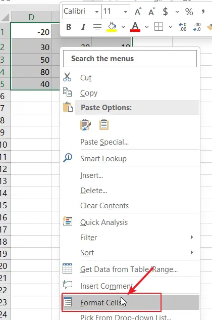
Step1: Select one range that you want to format.

Step2: Right-click and select “Format Cells” from the context menu.

Step3: In the Format Cells dialog box, select the “Number” tab. Select “Custom” from the Category list. In the “Type” field, enter the following format code: 0;[White0 , Click “OK” to apply the formatting.

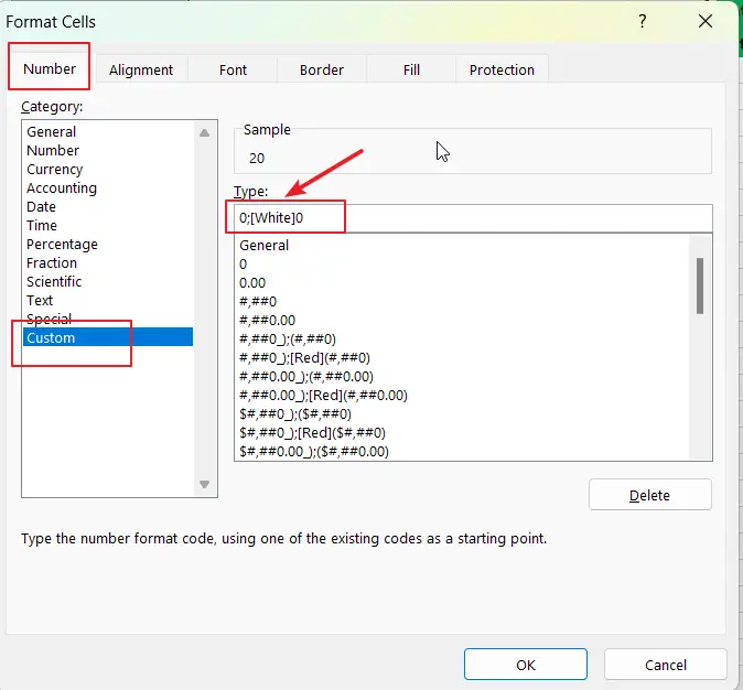
Step3: only positive numbers in the selected range will be displayed.

3. Show Only Positive Numbers in a Range with Conditional Formatting

If you only want to highlight or format positive numbers in a range, you can also use the Conditional Formatting feature in Microsoft Excel, just do the following steps:

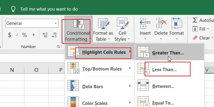
Step1: Select one range that want to format.

Step2: Click on the “Conditional Formatting” button in the “Home” tab of the ribbon. Select “Highlight Cell Rules” and then “Less Than” from the dropdown menu.

Step3: In the “Less Than” dialog box, enter “0” in the “Value” field. Choose “Custom Format…”, then set the font color as white.

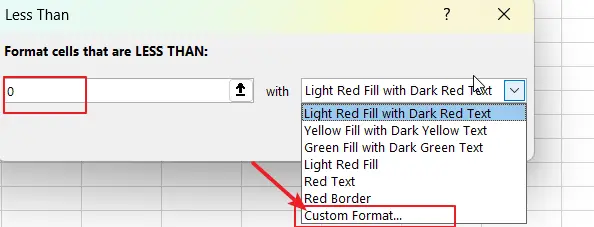
Step3: Click “OK” to apply the formatting.

This will only show all cells in the selected range that contain a value greater than zero.

4. Show Only Positive Numbers in a Range with VBA Code

If you want to show positive numbers in a range using VBA code, you can use a loop to iterate through each cell in the range and check if the value is greater than zero. If the value is positive, you can keep it in the cell. Otherwise, you can set font color as white.

Just refer to the following steps:

Step1: Press Alt + F11 on your keyboard. This will open the Visual Basic Editor.

Step2: Go to the menu bar at the top of the Visual Basic Editor and click on Insert -> Module. This will create a new module in the project.

Step3: Copy the following VBA code you want to run and paste it into the module. Save the VBA code and close the Visual Basic Editor.

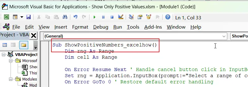
Sub ShowPositiveNumbers_excelhow()
    Dim rng As Range
    Dim cell As Range
    
    On Error Resume Next ' Handle cancel button click in InputBox
    Set rng = Application.InputBox(prompt:="Select a range of cells", Type:=8)
    On Error GoTo 0 ' Restore default error handling
    
    If Not rng Is Nothing Then ' Check if a range was selected
        For Each cell In rng
            If cell.Value < 0 Then
                cell.Font.Color = RGB(255, 255, 255)
            End If
        Next cell
    End If
End Sub

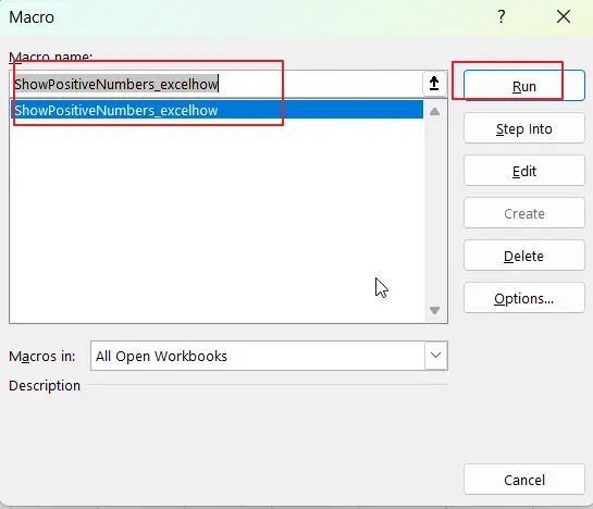
Step4: Press Alt + F8 to open the Macros dialog box. Select the macro you want to run and click on the Run button.

Step5: select a range of cells that you want to filter all positive values.

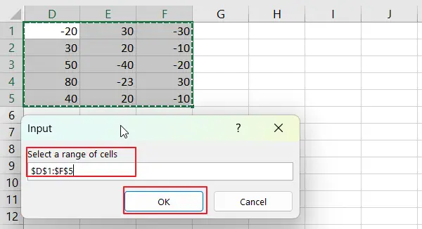
Step5: You can see that only positive values are shown in your selected range of cells.

5. Show Only Positive Values after Calculating

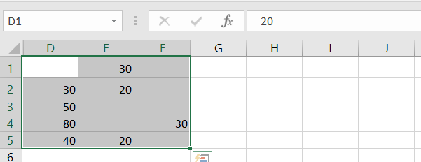
Assuming that you have a list of data, and you want to sum the range of cells A1:C5 and if the summation result is greater than 0 or is a positive number, then display this result. Otherwise, display as a blank cell.

You can create a formula based on the IF function, and the SUM function to sum all values in the range A1:C5 and just show only positive values. Like this:

=IF(SUM(A1:C1)<0, "",SUM(A1:C1))

Type this formula into the formula box of the cell D1, then drag AutoFill Handler over other cells to apply this formula.

show only positve values1

You will see that the returned results of this formula only show positive values.

Excel SUM function
The Excel SUM function will adds all numbers in a range of cells and returns the sum of these values. You can add individual values, cell references or ranges in excel.The syntax of the SUM function is as below:= SUM(number1,[number2],…)…
Excel IF function
The Excel IF function perform a logical test to return one value if the condition is TRUE and return another value if the condition is FALSE. The IF function is a build-in function in Microsoft Excel and it is categorized as a Logical Function.The syntax of the IF function is as below:= IF (condition, [true_value], [false_value])….

Источник

Data Validation is a feature in Microsoft Excel which restricts the values or type of data that users enter into a cell. It automatically checks whether the value entered is allowed based on the specified criteria. This step by step tutorial will assist all levels of Excel users in allowing unique values only.

Figure 1. Final result: Data validation unique values only

Working formula: =COUNTIF(C$3:C$7,C3)<2

Syntax of COUNTIF Function

COUNTIF returns the count or number of values in a specified range based on a given condition

=COUNTIF(range,criteria)

range – the data range that will be evaluated using the criteria
criteria – the criteria or condition that determines which cells will be counted

Setting up Our Data

Our table consists of two columns: Name (column B) and Student ID(column C). We want to ensure that a Student ID is unique to each student. We can restrict the values entered in column C and allow unique values only by applying Data Validation.

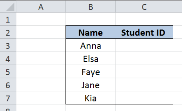Figure 2. Sample data: Data validation unique values only

We want to restrict the Student IDs entered in column C to be unique for each student. We can do this with Data Validation by following these steps:

Step 1. Select the cells whose values we want to restrict. In this case, select cells C3:C7

Step 2. Click the Data tab, then the Data Validation menu and select Data Validation

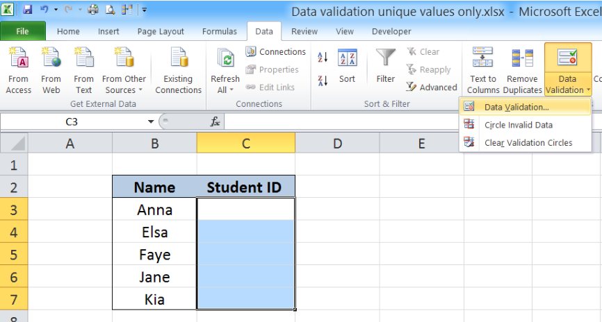Figure 3. Selecting Data Validation

The Data Validation dialog box will pop up.

Figure 4. Data Validation preview

Step 3. Click the Allow: drop-down button and select Custom as Validation criteria

Step 4. Enter the following in the Formula bar: =COUNTIF(C$3:C$7,C3)<2

The dollar signs “$” are necessary to fix specific cells in our formula and enable the validation criteria to work properly for all selected cells.

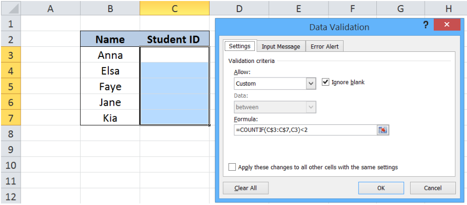Figure 5. Creating a data validation rule

Our COUNTIF function returns the count of the value in C3 within the range C3:C7. Our formula checks if the value entered in C3 does not already exist in the range C3:C7.

If the formula returns a count less than “2”, specifically “0” or “1”, Data Validation passes and the value is allowed. Otherwise, Data Validation fails and the value is restricted.

Step 5. Click OK

We have now restricted the values in C3:C7 to allow only unique values. Let us try and enter “19001” into cell C3.

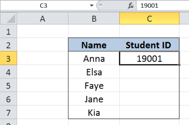Figure 6. Unique value “19001” allowed by Data Validation

The Student ID “19001” is allowed because it is unique in column C, and no other value is entered yet. Now let’s input “19001” into cell C4.

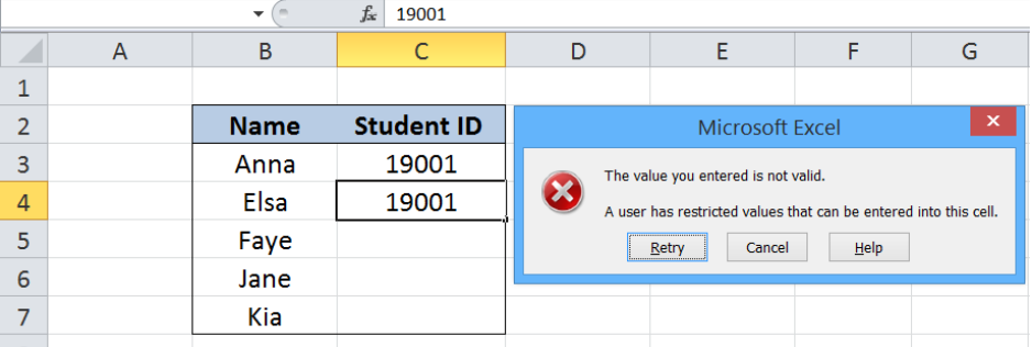Figure 7. ID “19001” entered twice and restricted by Data Validation

This time, the COUNTIF formula returns the count of 2 for “19001”, which exists in both cells C3 and C4. Hence, Data Validation fails and restricts the input of “19001” into cell C4. For restricted values, Excel shows a default warning message that says:

“The value you entered is not valid. A user has restricted values that can be entered into this cell.”

We are then presented with three options: Retry, Cancel or seek Help.

Data Validation is very accurate in allowing only the values as specified in the formula or validation criteria. See below table that is filled up with Student IDs unique to each student, as allowed by Data Validation.

Figure 8. Output: Data validation unique values only

Most of the time, the problem you will need to solve will be more complex than a simple application of a formula or function. If you want to save hours of research and frustration, try our live Excelchat service! Our Excel Experts are available 24/7 to answer any Excel question you may have. We guarantee a connection within 30 seconds and a customized solution within 20 minutes.

Источник

I have a table with month in one column and then sales in that month in the next column. Some months have no sales. I want to create a new table based using formulas so I only see the months with sales along with their sales. Such that;

Apr — 500
May — 500
June —
July —
Aug — 500

etc becomes

Apr — 500
May — 500
Aug — 500

asked May 21, 2020 at 15:40

Use the FILTER function:

The formula in cell I1:

=FILTER(F1:G5,G1:G5<>"")

EDIT:

If you don’t have the FILTER function, you can use an Advanced Filter on the «Sort & Filter» group on the Data tab on the Ribbon.

Configure a small filter table, which include a column without a header that has a formula that refers to a cell in the amount column in your data. The formula in cell K2 in the screenshot below is:

=G2<>""

answered May 21, 2020 at 16:38

FlexYourDataFlexYourData

6,2252 gold badges6 silver badges20 bronze badges

For older versions use INDEX/AGGREGATE:

=IFERROR(INDEX(A:A,AGGREGATE(15,7,ROW(A$1:A$5)/($B$1:$B$5<>""),ROW(A1))),"")

Put that in the first cell and copy over one column and down till you get blanks.

answered May 21, 2020 at 22:16

Scott CranerScott Craner

22.2k3 gold badges21 silver badges24 bronze badges

You need an Array (CSE) formula:

Formula in cell Q36:

{=IFERROR(INDEX(N$36:N$43,SMALL(IF($O$36:$O$43<>"",ROW($O$36:$O$43)-ROW($O$36)+1),ROWS(Q$35:Q35))),"")}

Finish formula with Ctrl+Shift+Enter & fill across.

:Edited:

 {=SMALL(IF(O$36:O$43<>"",ROW(O$36:O$43)-ROW(O$36)+1),ROWS(Q$35:Q35))}

Above formula, if is an array formula, then returns Row number of non blanks values from O36 to O43, otherwise gets only the first value’s Row number 1.

Check this explains that, how it works.

An Array (CSE) formula in cell V36:

{=SMALL(IF(O$36:O$43<>"",ROW(O$36:O$43)-ROW(O$36)+1),ROWS(V$35:V35))}

Formula in cell W36:

=INDEX(N$36:N$43,$V36)
Gets correct month name match with non blank cells, where INDEX gets order from V36 to V40.

And if you fill it Right then Down you get,

IFERROR replaces #NUM error with blanks.

So that the proper combination of INDEX and SMALL gets the month’s name along with related values in desire order.

Adjust cell references in all above formula as needed.

answered May 22, 2020 at 7:53

Rajesh SinhaRajesh Sinha

8,8926 gold badges15 silver badges35 bronze badges

Use a pivot table.

Step 1: create pivot table

Step 2: go to row labels -> value filters -> does not equal

Step 3: enter 0

Step 4: click ok, your pivot table should now look like this:

answered May 28, 2020 at 17:17

gns100gns100

9625 silver badges5 bronze badges

Источник

In this article, we will learn How to Only Return Results from Non-Blank Cells in Microsoft Excel.

What is a blank and non blank cell in Excel?

In Excel, Sometimes we don’t even want blank cells to disturb the formula. Most of the time we don’t want to work with a blank cell as it creates errors using the function. For Example VLOOKUP function returns #NA error when match type value is left blank. There are many functions like ISERROR which treats errors, but In this case we know the error is because of an empty value. So We learn the ISBLANK function in a formula with IF function.

IF — ISBLANK formula in Excel

ISBLANK function returns TRUE or FALSE boolean values based on the condition that the cell reference used is blank or not. Then use the required formula in the second or third argument.

Syntax of formula:

=IF(ISBLANK(cell_ref),[formula_if_blank],[ formula_if_false]

Cell ref : cell to check, if cell is blank or not.

Formula_if_true : formula or value if the cell is blank. Use Empty value («») if you want empty cell in return

Formula_if_false : formula or value if the cell is not blank. Use Empty value («») if you want empty cell in return

Example :

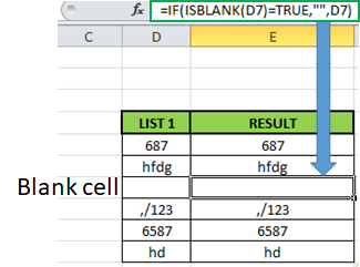
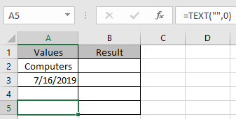
All of these might be confusing to understand. Let’s understand how to use the function using an example. Here we have some values on list 1 and we only want the formula to return the same value if not blank and empty value if blank.

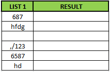
Formula:

=IF(ISBLANK(D5)=TRUE,«», D5)

Explanation:

ISBLANK : function checks the cell D5.

«» : returns an empty string blank cell instead of Zero.

IF function performs a logic_test if the test is true, it returns an empty string else returns the same value.

The resulting output will be like

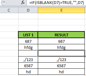
As you can see the formula returns the same value or blank cell based on the logic_test.

ISBLANK function with example

ISBLANK function returns TRUE or FALSE having cell reference as input.

Syntax:

Cell_ref : cell reference of cell to check e.g. B3

All of these might be confusing to understand. Let’s understand how to use the function using an example. Here We have some Values to test the function, except in the A5 cell. A5 cell has a formula that returns empty text.

Use the Formula

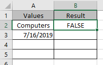
It returns False as there is text in the A2 cell.

Applying the formula in other cells using Ctrl + D shortcut key.

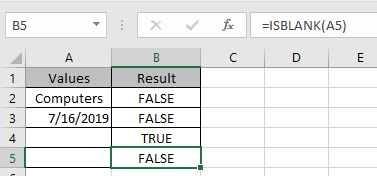
You must be wondering why didn’t the function returns False. As A5 cell has a formula making it non blank.

Hope this article about How to Only Return Results from Non-Blank Cells in Microsoft Excel is explanatory. Find more articles on blank values and related Excel formulas here. If you liked our blogs, share it with your friends on Facebook. And also you can follow us on Twitter and Facebook. We would love to hear from you, do let us know how we can improve, complement or innovate our work and make it better for you. Write to us at info@exceltip.com.

Related Articles :

Adjusting a Formula to Return a Blank : Formula adjusts its result on the basis of whether the cell is blank or not. Click the link to know how to use ISBLANK function with IF function in Excel.

Checking Whether Cells in a Range are Blank, and Counting the Blank Cells : If cells in a range are blank and calculating the blank cells in Excel then follow the link to understand more.

How to Calculate Only If Cell is Not Blank in Excel : Calculate only and only if the cell is not blank then use ISBLANK function in Excel.

Delete drop down list in Excel : The dropdown list is used to restrict the user to input data and gives the option to select from the list. We need to delete or remove the Dropdown list as the user will be able to input any data instead of choosing from a list.

Deleting All Cell Comments in Excel 2016 : Comments in Excel to remind ourselves and inform someone else about what the cell contains. To add the comment in a cell, Excel 2016 provides the insert Comment function. After inserting the comment it is displayed with little red triangles.

How to Delete only Filtered Rows without the Hidden Rows in Excel :Many of you are asking how to delete the selected rows without disturbing the other rows. We will use the Find & Select option in Excel.

How to Delete Sheets Without Confirmation Prompts Using VBA In Excel :There are times when we have to create or add sheets and later on we find no use of that sheet, hence we get the need to delete sheets quickly from the workbook

Popular Articles :

How to use the IF Function in Excel : The IF statement in Excel checks the condition and returns a specific value if the condition is TRUE or returns another specific value if FALSE.

How to use the VLOOKUP Function in Excel : This is one of the most used and popular functions of excel that is used to lookup value from different ranges and sheets.

How to use the SUMIF Function in Excel : This is another dashboard essential function. This helps you sum up values on specific conditions.

How to use the COUNTIF Function in Excel : Count values with conditions using this amazing function. You don’t need to filter your data to count specific values. Countif function is essential to prepare your dashboard.

Источник