
Excel for Microsoft 365 Excel for Microsoft 365 for Mac Excel for the web Excel 2021 Excel 2021 for Mac Excel 2019 Excel 2019 for Mac Excel 2016 Excel 2016 for Mac Excel 2013 Excel for iPad Excel for iPhone Excel for Android tablets Excel 2010 Excel 2007 Excel for Mac 2011 Excel for Android phones Excel Starter 2010 More…Less
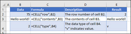
The CELL function returns information about the formatting, location, or contents of a cell. For example, if you want to verify that a cell contains a numeric value instead of text before you perform a calculation on it, you can use the following formula:
=IF(CELL(«type»,A1)=»v»,A1*2,0)
This formula calculates A1*2 only if cell A1 contains a numeric value, and returns 0 if A1 contains text or is blank.
Note: Formulas that use CELL have language-specific argument values and will return errors if calculated using a different language version of Excel. For example, if you create a formula containing CELL while using the Czech version of Excel, that formula will return an error if the workbook is opened using the French version. If it is important for others to open your workbook using different language versions of Excel, consider either using alternative functions or allowing others to save local copies in which they revise the CELL arguments to match their language.
Syntax
CELL(info_type, [reference])
The CELL function syntax has the following arguments:
|
Argument |
Description |
|---|---|
|
info_type Required |
A text value that specifies what type of cell information you want to return. The following list shows the possible values of the Info_type argument and the corresponding results. |
|
reference Optional |
The cell that you want information about. If omitted, the information specified in the info_type argument is returned for cell selected at the time of calculation. If the reference argument is a range of cells, the CELL function returns the information for active cell in the selected range. Important: Although technically reference is optional, including it in your formula is encouraged, unless you understand the effect its absence has on your formula result and want that effect in place. Omitting the reference argument does not reliably produce information about a specific cell, for the following reasons:
|
info_type values
The following list describes the text values that can be used for the info_type argument. These values must be entered in the CELL function with quotes (» «).
|
info_type |
Returns |
|---|---|
|
«address» |
Reference of the first cell in reference, as text. |
|
«col» |
Column number of the cell in reference. |
|
«color» |
The value 1 if the cell is formatted in color for negative values; otherwise returns 0 (zero). Note: This value is not supported in Excel for the web, Excel Mobile, and Excel Starter. |
|
«contents» |
Value of the upper-left cell in reference; not a formula. |
|
«filename» |
Filename (including full path) of the file that contains reference, as text. Returns empty text («») if the worksheet that contains reference has not yet been saved. Note: This value is not supported in Excel for the web, Excel Mobile, and Excel Starter. |
|
«format» |
Text value corresponding to the number format of the cell. The text values for the various formats are shown in the following table. Returns «-» at the end of the text value if the cell is formatted in color for negative values. Returns «()» at the end of the text value if the cell is formatted with parentheses for positive or all values. Note: This value is not supported in Excel for the web, Excel Mobile, and Excel Starter. |
|
«parentheses» |
The value 1 if the cell is formatted with parentheses for positive or all values; otherwise returns 0. Note: This value is not supported in Excel for the web, Excel Mobile, and Excel Starter. |
|
«prefix» |
Text value corresponding to the «label prefix» of the cell. Returns single quotation mark (‘) if the cell contains left-aligned text, double quotation mark («) if the cell contains right-aligned text, caret (^) if the cell contains centered text, backslash () if the cell contains fill-aligned text, and empty text («») if the cell contains anything else. Note: This value is not supported in Excel for the web, Excel Mobile, and Excel Starter. |
|
«protect» |
The value 0 if the cell is not locked; otherwise returns 1 if the cell is locked. Note: This value is not supported in Excel for the web, Excel Mobile, and Excel Starter. |
|
«row» |
Row number of the cell in reference. |
|
«type» |
Text value corresponding to the type of data in the cell. Returns «b» for blank if the cell is empty, «l» for label if the cell contains a text constant, and «v» for value if the cell contains anything else. |
|
«width» |
Returns an array with 2 items. The 1st item in the array is the column width of the cell, rounded off to an integer. Each unit of column width is equal to the width of one character in the default font size. The 2nd item in the array is a Boolean value, the value is TRUE if the column width is the default or FALSE if the width has been explicitly set by the user. Note: This value is not supported in Excel for the web, Excel Mobile, and Excel Starter. |
CELL format codes
The following list describes the text values that the CELL function returns when the Info_type argument is «format» and the reference argument is a cell that is formatted with a built-in number format.
|
If the Excel format is |
The CELL function returns |
|---|---|
|
General |
«G» |
|
0 |
«F0» |
|
#,##0 |
«,0» |
|
0.00 |
«F2» |
|
#,##0.00 |
«,2» |
|
$#,##0_);($#,##0) |
«C0» |
|
$#,##0_);[Red]($#,##0) |
«C0-« |
|
$#,##0.00_);($#,##0.00) |
«C2» |
|
$#,##0.00_);[Red]($#,##0.00) |
«C2-« |
|
0% |
«P0» |
|
0.00% |
«P2» |
|
0.00E+00 |
«S2» |
|
# ?/? or # ??/?? |
«G» |
|
m/d/yy or m/d/yy h:mm or mm/dd/yy |
«D4» |
|
d-mmm-yy or dd-mmm-yy |
«D1» |
|
d-mmm or dd-mmm |
«D2» |
|
mmm-yy |
«D3» |
|
mm/dd |
«D5» |
|
h:mm AM/PM |
«D7» |
|
h:mm:ss AM/PM |
«D6» |
|
h:mm |
«D9» |
|
h:mm:ss |
«D8» |
Note: If the info_type argument in the CELL function is «format» and you later apply a different format to the referenced cell, you must recalculate the worksheet (press F9) to update the results of the CELL function.
Examples
Need more help?
You can always ask an expert in the Excel Tech Community or get support in the Answers community.
See Also
Change the format of a cell
Create or change a cell reference
ADDRESS function
Add, change, find or clear conditional formatting in a cell
Need more help?
Want more options?
Explore subscription benefits, browse training courses, learn how to secure your device, and more.
Communities help you ask and answer questions, give feedback, and hear from experts with rich knowledge.
Return to Excel Formulas List
Download Example Workbook
Download the example workbook
This tutorial demonstrates how to get a cell value using the address of the cell (row and column) in Excel and Google Sheets.
Get Cell Value With the INDEX Function
We can get the value of a cell (its content) by using the INDEX Function.
The INDEX Function looks up a cell contained within a specified range and returns its value.
=INDEX(A1:J10,C3,C4)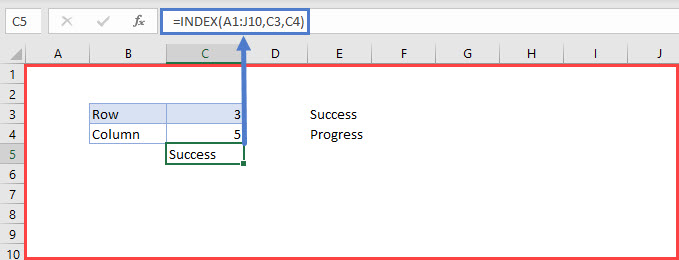
In the example above, the range specified in the INDEX formula is “A1:J10”, the row is cell “C3” (“3”), and the column is cell “C4” (“5”).
The formula looks through the range “A1:J10”, checks the cell in Row 3 and Column 5 (“E3”) and returns its value (“Success”).
Get Cell Value With the INDIRECT Function
Another option for getting the value of a cell by its address is to use the INDIRECT Function.
We can use the INDIRECT Function here in two different ways.
Using Text Reference Within the INDIRECT Function
The INDIRECT Function changes a specified text string to a cell reference and returns its value.
=INDIRECT("R" & 3 & "C" & 2,FALSE)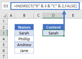
In the example above, the specified text string is “R3C2”. This means Row 3, Column 2. So the formula returns the value in that address (“Sarah”).
Note: The FALSE argument in this formula indicates the cell reference format (R1C1). (TRUE would use A1 style cell referencing).
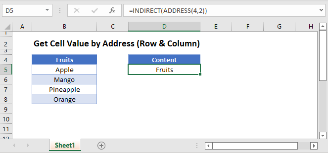
Get Cell Value by Using INDIRECT and ADDRESS
The second way to get the value of a cell using the INDIRECT Function is to combine it with the ADDRESS Function.
=INDIRECT(ADDRESS(4,2))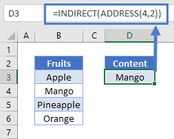
Let’s breakdown the formula into steps.
=ADDRESS(4,2)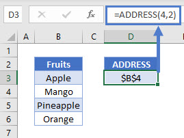
The ADDRESS Function takes a specified row number (“4”) and column number (“2”) and returns its absolute reference (“$B$4”). Therefore, the absolute reference for the cell in Column 2 (Column B based on position) and Row 4 is $B$4.
The INDIRECT Function returns the value of the cell referenced.
=INDIRECT(D3)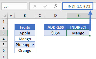
Combining these steps gives us our initial formula:
=INDIRECT(ADDRESS(4,2))
Note: The INDIRECT Function is volatile. It recalculates every time the workbook does and can cause Excel to run slowly. We recommend avoiding the use of large numbers of INDIRECT Functions in your workbooks.
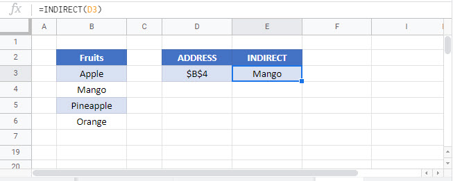
Get Cell Value by Address in Google Sheets
These formulas work exactly the same in Google Sheets as in Excel.
На чтение 18 мин. Просмотров 74.9k.

сэр Артур Конан Дойл
Это большая ошибка — теоретизировать, прежде чем кто-то получит данные
Эта статья охватывает все, что вам нужно знать об использовании ячеек и диапазонов в VBA. Вы можете прочитать его от начала до конца, так как он сложен в логическом порядке. Или использовать оглавление ниже, чтобы перейти к разделу по вашему выбору.
Рассматриваемые темы включают свойство смещения, чтение
значений между ячейками, чтение значений в массивы и форматирование ячеек.
Содержание
- Краткое руководство по диапазонам и клеткам
- Введение
- Важное замечание
- Свойство Range
- Свойство Cells рабочего листа
- Использование Cells и Range вместе
- Свойство Offset диапазона
- Использование диапазона CurrentRegion
- Использование Rows и Columns в качестве Ranges
- Использование Range вместо Worksheet
- Чтение значений из одной ячейки в другую
- Использование метода Range.Resize
- Чтение Value в переменные
- Как копировать и вставлять ячейки
- Чтение диапазона ячеек в массив
- Пройти через все клетки в диапазоне
- Форматирование ячеек
- Основные моменты
Краткое руководство по диапазонам и клеткам
| Функция | Принимает | Возвращает | Пример | Вид |
| Range | адреса ячеек |
диапазон ячеек |
.Range(«A1:A4») | $A$1:$A$4 |
| Cells | строка, столбец |
одна ячейка |
.Cells(1,5) | $E$1 |
| Offset | строка, столбец |
диапазон | .Range(«A1:A2») .Offset(1,2) |
$C$2:$C$3 |
| Rows | строка (-и) | одна или несколько строк |
.Rows(4) .Rows(«2:4») |
$4:$4 $2:$4 |
| Columns | столбец (-цы) |
один или несколько столбцов |
.Columns(4) .Columns(«B:D») |
$D:$D $B:$D |
Введение
Это третья статья, посвященная трем основным элементам VBA. Этими тремя элементами являются Workbooks, Worksheets и Ranges/Cells. Cells, безусловно, самая важная часть Excel. Почти все, что вы делаете в Excel, начинается и заканчивается ячейками.
Вы делаете три основных вещи с помощью ячеек:
- Читаете из ячейки.
- Пишите в ячейку.
- Изменяете формат ячейки.
В Excel есть несколько методов для доступа к ячейкам, таких как Range, Cells и Offset. Можно запутаться, так как эти функции делают похожие операции.
В этой статье я расскажу о каждом из них, объясню, почему они вам нужны, и когда вам следует их использовать.
Давайте начнем с самого простого метода доступа к ячейкам — с помощью свойства Range рабочего листа.
Важное замечание
Я недавно обновил эту статью, сейчас использую Value2.
Вам может быть интересно, в чем разница между Value, Value2 и значением по умолчанию:
' Value2
Range("A1").Value2 = 56

' Value
Range("A1").Value = 56

' По умолчанию используется значение
Range("A1") = 56
Использование Value может усечь число, если ячейка отформатирована, как валюта. Если вы не используете какое-либо свойство, по умолчанию используется Value.
Лучше использовать Value2, поскольку он всегда будет возвращать фактическое значение ячейки.
Свойство Range
Рабочий лист имеет свойство Range, которое можно использовать для доступа к ячейкам в VBA. Свойство Range принимает тот же аргумент, что и большинство функций Excel Worksheet, например: «А1», «А3: С6» и т.д.
В следующем примере показано, как поместить значение в ячейку с помощью свойства Range.
Sub ZapisVYacheiku()

    ' Запишите число в ячейку A1 на листе 1 этой книги
    ThisWorkbook.Worksheets("Лист1").Range("A1").Value2 = 67

    ' Напишите текст в ячейку A2 на листе 1 этой рабочей книги
    ThisWorkbook.Worksheets("Лист1").Range("A2").Value2 = "Иван Петров"

    ' Запишите дату в ячейку A3 на листе 1 этой книги
    ThisWorkbook.Worksheets("Лист1").Range("A3").Value2 = #11/21/2019#

End Sub
Как видно из кода, Range является членом Worksheets, которая, в свою очередь, является членом Workbook. Иерархия такая же, как и в Excel, поэтому должно быть легко понять. Чтобы сделать что-то с Range, вы должны сначала указать рабочую книгу и рабочий лист, которому она принадлежит.
В оставшейся части этой статьи я буду использовать кодовое имя для ссылки на лист.

Следующий код показывает приведенный выше пример с использованием кодового имени рабочего листа, т.е. Лист1 вместо ThisWorkbook.Worksheets («Лист1»).
Sub IspKodImya ()

    ' Запишите число в ячейку A1 на листе 1 этой книги
     Sheet1.Range("A1").Value2 = 67

    ' Напишите текст в ячейку A2 на листе 1 этой рабочей книги
    Sheet1.Range("A2").Value2 = "Иван Петров"

    ' Запишите дату в ячейку A3 на листе 1 этой книги
    Sheet1.Range("A3").Value2 = #11/21/2019#

End Sub
Вы также можете писать в несколько ячеек, используя свойство
Range
Sub ZapisNeskol()

    ' Запишите число в диапазон ячеек
    Sheet1.Range("A1:A10").Value2 = 67

    ' Написать текст в несколько диапазонов ячеек
    Sheet1.Range("B2:B5,B7:B9").Value2 = "Иван Петров"

End Sub
Свойство Cells рабочего листа
У Объекта листа есть другое свойство, называемое Cells, которое очень похоже на Range . Есть два отличия:
- Cells возвращают диапазон только одной ячейки.
- Cells принимает строку и столбец в качестве аргументов.
В приведенном ниже примере показано, как записывать значения
в ячейки, используя свойства Range и Cells.
Sub IspCells()

    ' Написать в А1
    Sheet1.Range("A1").Value2 = 10
    Sheet1.Cells(1, 1).Value2  = 10

    ' Написать в А10
    Sheet1.Range("A10").Value2 = 10
    Sheet1.Cells(10, 1).Value2  = 10

    ' Написать в E1
    Sheet1.Range("E1").Value2 = 10
    Sheet1.Cells(1, 5).Value2  = 10

End Sub
Вам должно быть интересно, когда использовать Cells, а когда Range. Использование Range полезно для доступа к одним и тем же ячейкам при каждом запуске макроса.
Например, если вы использовали макрос для вычисления суммы и
каждый раз записывали ее в ячейку A10, тогда Range подойдет для этой задачи.
Использование свойства Cells полезно, если вы обращаетесь к
ячейке по номеру, который может отличаться. Проще объяснить это на примере.
В следующем коде мы просим пользователя указать номер столбца. Использование Cells дает нам возможность использовать переменное число для столбца.
Sub ZapisVPervuyuPustuyuYacheiku()

    Dim UserCol As Integer

    ' Получить номер столбца от пользователя
    UserCol = Application.InputBox("Пожалуйста, введите номер столбца...", Type:=1)

    ' Написать текст в выбранный пользователем столбец
    Sheet1.Cells(1, UserCol).Value2 = "Иван Петров"

End Sub
В приведенном выше примере мы используем номер для столбца,
а не букву.
Чтобы использовать Range здесь, потребуется преобразовать эти значения в ссылку на
буквенно-цифровую ячейку, например, «С1». Использование свойства Cells позволяет нам
предоставить строку и номер столбца для доступа к ячейке.
Иногда вам может понадобиться вернуть более одной ячейки, используя номера строк и столбцов. В следующем разделе показано, как это сделать.
Использование Cells и Range вместе
Как вы уже видели, вы можете получить доступ только к одной ячейке, используя свойство Cells. Если вы хотите вернуть диапазон ячеек, вы можете использовать Cells с Range следующим образом:
Sub IspCellsSRange()

    With Sheet1
        ' Запишите 5 в диапазон A1: A10, используя свойство Cells
        .Range(.Cells(1, 1), .Cells(10, 1)).Value2 = 5

        ' Диапазон B1: Z1 будет выделен жирным шрифтом
        .Range(.Cells(1, 2), .Cells(1, 26)).Font.Bold = True

    End With

End Sub
Как видите, вы предоставляете начальную и конечную ячейку
диапазона. Иногда бывает сложно увидеть, с каким диапазоном вы имеете дело,
когда значением являются все числа. Range имеет свойство Address, которое
отображает буквенно-цифровую ячейку для любого диапазона. Это может
пригодиться, когда вы впервые отлаживаете или пишете код.
В следующем примере мы распечатываем адрес используемых нами
диапазонов.
Sub PokazatAdresDiapazona()

    ' Примечание. Использование подчеркивания позволяет разделить строки кода.
    With Sheet1

        ' Запишите 5 в диапазон A1: A10, используя свойство Cells
        .Range(.Cells(1, 1), .Cells(10, 1)).Value2 = 5
        Debug.Print "Первый адрес: " _
            + .Range(.Cells(1, 1), .Cells(10, 1)).Address

        ' Диапазон B1: Z1 будет выделен жирным шрифтом
        .Range(.Cells(1, 2), .Cells(1, 26)).Font.Bold = True
        Debug.Print "Второй адрес : " _
            + .Range(.Cells(1, 2), .Cells(1, 26)).Address

    End With

End Sub
В примере я использовал Debug.Print для печати в Immediate Window. Для просмотра этого окна выберите «View» -> «в Immediate Window» (Ctrl + G).


Свойство Offset диапазона
У диапазона есть свойство, которое называется Offset. Термин «Offset» относится к отсчету от исходной позиции. Он часто используется в определенных областях программирования. С помощью свойства «Offset» вы можете получить диапазон ячеек того же размера и на определенном расстоянии от текущего диапазона. Это полезно, потому что иногда вы можете выбрать диапазон на основе определенного условия. Например, на скриншоте ниже есть столбец для каждого дня недели. Учитывая номер дня (т.е. понедельник = 1, вторник = 2 и т.д.). Нам нужно записать значение в правильный столбец.

Сначала мы попытаемся сделать это без использования Offset.
' Это Sub тесты с разными значениями
Sub TestSelect()

    ' Понедельник
    SetValueSelect 1, 111.21
    ' Среда
    SetValueSelect 3, 456.99
    ' Пятница
    SetValueSelect 5, 432.25
    ' Воскресение
    SetValueSelect 7, 710.17

End Sub

' Записывает значение в столбец на основе дня
Public Sub SetValueSelect(lDay As Long, lValue As Currency)

    Select Case lDay
        Case 1: Sheet1.Range("H3").Value2 = lValue
        Case 2: Sheet1.Range("I3").Value2 = lValue
        Case 3: Sheet1.Range("J3").Value2 = lValue
        Case 4: Sheet1.Range("K3").Value2 = lValue
        Case 5: Sheet1.Range("L3").Value2 = lValue
        Case 6: Sheet1.Range("M3").Value2 = lValue
        Case 7: Sheet1.Range("N3").Value2 = lValue
    End Select

End Sub
Как видно из примера, нам нужно добавить строку для каждого возможного варианта. Это не идеальная ситуация. Использование свойства Offset обеспечивает более чистое решение.
' Это Sub тесты с разными значениями
Sub TestOffset()

    DayOffSet 1, 111.01
    DayOffSet 3, 456.99
    DayOffSet 5, 432.25
    DayOffSet 7, 710.17

End Sub

Public Sub DayOffSet(lDay As Long, lValue As Currency)

    ' Мы используем значение дня с Offset, чтобы указать правильный столбец
    Sheet1.Range("G3").Offset(, lDay).Value2 = lValue

End Sub
Как видите, это решение намного лучше. Если количество дней увеличилось, нам больше не нужно добавлять код. Чтобы Offset был полезен, должна быть какая-то связь между позициями ячеек. Если столбцы Day в приведенном выше примере были случайными, мы не могли бы использовать Offset. Мы должны были бы использовать первое решение.
Следует иметь в виду, что Offset сохраняет размер диапазона. Итак .Range («A1:A3»).Offset (1,1) возвращает диапазон B2:B4. Ниже приведены еще несколько примеров использования Offset.
Sub IspOffset()

    ' Запись в В2 - без Offset
    Sheet1.Range("B2").Offset().Value2 = "Ячейка B2"

    ' Написать в C2 - 1 столбец справа
    Sheet1.Range("B2").Offset(, 1).Value2 = "Ячейка C2"

    ' Написать в B3 - 1 строка вниз
    Sheet1.Range("B2").Offset(1).Value2 = "Ячейка B3"

    ' Запись в C3 - 1 столбец справа и 1 строка вниз
    Sheet1.Range("B2").Offset(1, 1).Value2 = "Ячейка C3"

    ' Написать в A1 - 1 столбец слева и 1 строка вверх
    Sheet1.Range("B2").Offset(-1, -1).Value2 = "Ячейка A1"

    ' Запись в диапазон E3: G13 - 1 столбец справа и 1 строка вниз
    Sheet1.Range("D2:F12").Offset(1, 1).Value2 = "Ячейки E3:G13"

End Sub
Использование диапазона CurrentRegion
CurrentRegion возвращает диапазон всех соседних ячеек в данный диапазон. На скриншоте ниже вы можете увидеть два CurrentRegion. Я добавил границы, чтобы прояснить CurrentRegion.

Строка или столбец пустых ячеек означает конец CurrentRegion.
Вы можете вручную проверить
CurrentRegion в Excel, выбрав диапазон и нажав Ctrl + Shift + *.
Если мы возьмем любой диапазон
ячеек в пределах границы и применим CurrentRegion, мы вернем диапазон ячеек во
всей области.
Например:
Range («B3»). CurrentRegion вернет диапазон B3:D14
Range («D14»). CurrentRegion вернет диапазон B3:D14
Range («C8:C9»). CurrentRegion вернет диапазон B3:D14 и так далее
Как пользоваться
Мы получаем CurrentRegion следующим образом
' CurrentRegion вернет B3:D14 из приведенного выше примера
Dim rg As Range
Set rg = Sheet1.Range("B3").CurrentRegion
Только чтение строк данных
Прочитать диапазон из второй строки, т.е. пропустить строку заголовка.
' CurrentRegion вернет B3:D14 из приведенного выше примера
Dim rg As Range
Set rg = Sheet1.Range("B3").CurrentRegion

' Начало в строке 2 - строка после заголовка
Dim i As Long
For i = 2 To rg.Rows.Count
    ' текущая строка, столбец 1 диапазона
    Debug.Print rg.Cells(i, 1).Value2
Next i
Удалить заголовок
Удалить строку заголовка (т.е. первую строку) из диапазона. Например, если диапазон — A1:D4, это возвратит A2:D4
' CurrentRegion вернет B3:D14 из приведенного выше примера
Dim rg As Range
Set rg = Sheet1.Range("B3").CurrentRegion

' Удалить заголовок
Set rg = rg.Resize(rg.Rows.Count - 1).Offset(1)

' Начните со строки 1, так как нет строки заголовка
Dim i As Long
For i = 1 To rg.Rows.Count
    ' текущая строка, столбец 1 диапазона
    Debug.Print rg.Cells(i, 1).Value2
Next i
Использование Rows и Columns в качестве Ranges
Если вы хотите что-то сделать со всей строкой или столбцом,
вы можете использовать свойство «Rows и
Columns» на рабочем листе. Они оба принимают один параметр — номер строки
или столбца, к которому вы хотите получить доступ.
Sub IspRowIColumns()

    ' Установите размер шрифта столбца B на 9
    Sheet1.Columns(2).Font.Size = 9

    ' Установите ширину столбцов от D до F
    Sheet1.Columns("D:F").ColumnWidth = 4

    ' Установите размер шрифта строки 5 до 18
    Sheet1.Rows(5).Font.Size = 18

End Sub
Использование Range вместо Worksheet
Вы также можете использовать Cella, Rows и Columns, как часть Range, а не как часть Worksheet. У вас может быть особая необходимость в этом, но в противном случае я бы избегал практики. Это делает код более сложным. Простой код — твой друг. Это уменьшает вероятность ошибок.
Код ниже выделит второй столбец диапазона полужирным. Поскольку диапазон имеет только две строки, весь столбец считается B1:B2
Sub IspColumnsVRange()

    ' Это выделит B1 и B2 жирным шрифтом.
    Sheet1.Range("A1:C2").Columns(2).Font.Bold = True

End Sub
Чтение значений из одной ячейки в другую
В большинстве примеров мы записали значения в ячейку. Мы
делаем это, помещая диапазон слева от знака равенства и значение для размещения
в ячейке справа. Для записи данных из одной ячейки в другую мы делаем то же
самое. Диапазон назначения идет слева, а диапазон источника — справа.
В следующем примере показано, как это сделать:
Sub ChitatZnacheniya()

    ' Поместите значение из B1 в A1
    Sheet1.Range("A1").Value2 = Sheet1.Range("B1").Value2

    ' Поместите значение из B3 в лист2 в ячейку A1
    Sheet1.Range("A1").Value2 = Sheet2.Range("B3").Value2

    ' Поместите значение от B1 в ячейки A1 до A5
    Sheet1.Range("A1:A5").Value2 = Sheet1.Range("B1").Value2

    ' Вам необходимо использовать свойство «Value», чтобы прочитать несколько ячеек
    Sheet1.Range("A1:A5").Value2 = Sheet1.Range("B1:B5").Value2

End Sub
Как видно из этого примера, невозможно читать из нескольких ячеек. Если вы хотите сделать это, вы можете использовать функцию копирования Range с параметром Destination.
Sub KopirovatZnacheniya()

    ' Сохранить диапазон копирования в переменной
    Dim rgCopy As Range
    Set rgCopy = Sheet1.Range("B1:B5")

    ' Используйте это для копирования из более чем одной ячейки
    rgCopy.Copy Destination:=Sheet1.Range("A1:A5")

    ' Вы можете вставить в несколько мест назначения
    rgCopy.Copy Destination:=Sheet1.Range("A1:A5,C2:C6")

End Sub
Функция Copy копирует все, включая формат ячеек. Это тот же результат, что и ручное копирование и вставка выделения. Подробнее об этом вы можете узнать в разделе «Копирование и вставка ячеек»
Использование метода Range.Resize
При копировании из одного диапазона в другой с использованием присваивания (т.е. знака равенства) диапазон назначения должен быть того же размера, что и исходный диапазон.
Использование функции Resize позволяет изменить размер
диапазона до заданного количества строк и столбцов.
Например:
Sub ResizePrimeri()

    ' Печатает А1
    Debug.Print Sheet1.Range("A1").Address

    ' Печатает A1:A2
    Debug.Print Sheet1.Range("A1").Resize(2, 1).Address

    ' Печатает A1:A5
    Debug.Print Sheet1.Range("A1").Resize(5, 1).Address

    ' Печатает A1:D1
    Debug.Print Sheet1.Range("A1").Resize(1, 4).Address

    ' Печатает A1:C3
    Debug.Print Sheet1.Range("A1").Resize(3, 3).Address

End Sub
Когда мы хотим изменить наш целевой диапазон, мы можем
просто использовать исходный размер диапазона.
Другими словами, мы используем количество строк и столбцов
исходного диапазона в качестве параметров для изменения размера:
Sub Resize()

    Dim rgSrc As Range, rgDest As Range

    ' Получить все данные в текущей области
    Set rgSrc = Sheet1.Range("A1").CurrentRegion

      ' Получить диапазон назначения
    Set rgDest = Sheet2.Range("A1")
    Set rgDest = rgDest.Resize(rgSrc.Rows.Count, rgSrc.Columns.Count)

    rgDest.Value2 = rgSrc.Value2

End Sub
Мы можем сделать изменение размера в одну строку, если нужно:
Sub Resize2()

    Dim rgSrc As Range

    ' Получить все данные в ткущей области
    Set rgSrc = Sheet1.Range("A1").CurrentRegion

    With rgSrc
        Sheet2.Range("A1").Resize(.Rows.Count, .Columns.Count) = .Value2
    End With

End Sub
Чтение Value в переменные
Мы рассмотрели, как читать из одной клетки в другую. Вы также можете читать из ячейки в переменную. Переменная используется для хранения значений во время работы макроса. Обычно вы делаете это, когда хотите манипулировать данными перед тем, как их записать. Ниже приведен простой пример использования переменной. Как видите, значение элемента справа от равенства записывается в элементе слева от равенства.
Sub IspVar()

    ' Создайте
    Dim val As Integer

    ' Читать число из ячейки
    val = Sheet1.Range("A1").Value2

    ' Добавить 1 к значению
    val = val + 1

    ' Запишите новое значение в ячейку
    Sheet1.Range("A2").Value2 = val

End Sub
Для чтения текста в переменную вы используете переменную
типа String.
Sub IspVarText()

    ' Объявите переменную типа string
    Dim sText As String

    ' Считать значение из ячейки
    sText = Sheet1.Range("A1").Value2

    ' Записать значение в ячейку
    Sheet1.Range("A2").Value2 = sText

End Sub
Вы можете записать переменную в диапазон ячеек. Вы просто
указываете диапазон слева, и значение будет записано во все ячейки диапазона.
Sub VarNeskol()

    ' Считать значение из ячейки
    Sheet1.Range("A1:B10").Value2 = 66

End Sub
Вы не можете читать из нескольких ячеек в переменную. Однако
вы можете читать массив, который представляет собой набор переменных. Мы
рассмотрим это в следующем разделе.
Как копировать и вставлять ячейки
Если вы хотите скопировать и вставить диапазон ячеек, вам не
нужно выбирать их. Это распространенная ошибка, допущенная новыми пользователями
VBA.
Вы можете просто скопировать ряд ячеек, как здесь:
Range("A1:B4").Copy Destination:=Range("C5")
При использовании этого метода копируется все — значения,
форматы, формулы и так далее. Если вы хотите скопировать отдельные элементы, вы
можете использовать свойство PasteSpecial
диапазона.
Работает так:
Range("A1:B4").Copy
Range("F3").PasteSpecial Paste:=xlPasteValues
Range("F3").PasteSpecial Paste:=xlPasteFormats
Range("F3").PasteSpecial Paste:=xlPasteFormulas
В следующей таблице приведен полный список всех типов вставок.
| Виды вставок |
| xlPasteAll |
| xlPasteAllExceptBorders |
| xlPasteAllMergingConditionalFormats |
| xlPasteAllUsingSourceTheme |
| xlPasteColumnWidths |
| xlPasteComments |
| xlPasteFormats |
| xlPasteFormulas |
| xlPasteFormulasAndNumberFormats |
| xlPasteValidation |
| xlPasteValues |
| xlPasteValuesAndNumberFormats |
Чтение диапазона ячеек в массив
Вы также можете скопировать значения, присвоив значение
одного диапазона другому.
Range("A3:Z3").Value2 = Range("A1:Z1").Value2
Значение диапазона в этом примере считается вариантом массива. Это означает, что вы можете легко читать из диапазона ячеек в массив. Вы также можете писать из массива в диапазон ячеек. Если вы не знакомы с массивами, вы можете проверить их в этой статье.
В следующем коде показан пример использования массива с
диапазоном.
Sub ChitatMassiv()

    ' Создать динамический массив
    Dim StudentMarks() As Variant

    ' Считать 26 значений в массив из первой строки
    StudentMarks = Range("A1:Z1").Value2

    ' Сделайте что-нибудь с массивом здесь

    ' Запишите 26 значений в третью строку
    Range("A3:Z3").Value2 = StudentMarks

End Sub
Имейте в виду, что массив, созданный для чтения, является
двумерным массивом. Это связано с тем, что электронная таблица хранит значения
в двух измерениях, то есть в строках и столбцах.
Пройти через все клетки в диапазоне
Иногда вам нужно просмотреть каждую ячейку, чтобы проверить значение.
Вы можете сделать это, используя цикл For Each, показанный в следующем коде.
Sub PeremeschatsyaPoYacheikam()

    ' Пройдите через каждую ячейку в диапазоне
    Dim rg As Range
    For Each rg In Sheet1.Range("A1:A10,A20")
        ' Распечатать адрес ячеек, которые являются отрицательными
        If rg.Value < 0 Then
            Debug.Print rg.Address + " Отрицательно."
        End If
    Next

End Sub
Вы также можете проходить последовательные ячейки, используя
свойство Cells и стандартный цикл For.
Стандартный цикл более гибок в отношении используемого вами
порядка, но он медленнее, чем цикл For Each.
Sub PerehodPoYacheikam()

    ' Пройдите клетки от А1 до А10
    Dim i As Long
    For i = 1 To 10
        ' Распечатать адрес ячеек, которые являются отрицательными
        If Range("A" & i).Value < 0 Then
            Debug.Print Range("A" & i).Address + " Отрицательно."
        End If
    Next

    ' Пройдите в обратном порядке, то есть от A10 до A1
    For i = 10 To 1 Step -1
        ' Распечатать адрес ячеек, которые являются отрицательными
        If Range("A" & i) < 0 Then
            Debug.Print Range("A" & i).Address + " Отрицательно."
        End If
    Next

End Sub
Форматирование ячеек
Иногда вам нужно будет отформатировать ячейки в электронной
таблице. Это на самом деле очень просто. В следующем примере показаны различные
форматы, которые можно добавить в любой диапазон ячеек.
Sub FormatirovanieYacheek()

    With Sheet1

        ' Форматировать шрифт
        .Range("A1").Font.Bold = True
        .Range("A1").Font.Underline = True
        .Range("A1").Font.Color = rgbNavy

        ' Установите числовой формат до 2 десятичных знаков
        .Range("B2").NumberFormat = "0.00"
        ' Установите числовой формат даты
        .Range("C2").NumberFormat = "dd/mm/yyyy"
        ' Установите формат чисел на общий
        .Range("C3").NumberFormat = "Общий"
        ' Установить числовой формат текста
        .Range("C4").NumberFormat = "Текст"

        ' Установите цвет заливки ячейки
        .Range("B3").Interior.Color = rgbSandyBrown

        ' Форматировать границы
        .Range("B4").Borders.LineStyle = xlDash
        .Range("B4").Borders.Color = rgbBlueViolet

    End With

End Sub
Основные моменты
Ниже приводится краткое изложение основных моментов
- Range возвращает диапазон ячеек
- Cells возвращают только одну клетку
- Вы можете читать из одной ячейки в другую
- Вы можете читать из диапазона ячеек в другой диапазон ячеек.
- Вы можете читать значения из ячеек в переменные и наоборот.
- Вы можете читать значения из диапазонов в массивы и наоборот
- Вы можете использовать цикл For Each или For, чтобы проходить через каждую ячейку в диапазоне.
- Свойства Rows и Columns позволяют вам получить доступ к диапазону ячеек этих типов
 Please Note:
This article is written for users of the following Microsoft Excel versions: 2007, 2010, 2013, 2016, 2019, and Excel in Microsoft 365. If you are using an earlier version (Excel 2003 or earlier), this tip may not work for you. For a version of this tip written specifically for earlier versions of Excel, click here: Determining a Value of a Cell.
![]()
Written by Allen Wyatt (last updated August 25, 2022)
This tip applies to Excel 2007, 2010, 2013, 2016, 2019, and Excel in Microsoft 365
You already know that a cell in a worksheet can contain any number of different items: numbers, dates, formulas, and so on. There may be times when you want to determine the underlying value in a cell, without regard to the way the cell is formatted. For this need, Excel provides the N worksheet function. For instance, let’s assume that cell F17 contains a date. If you use = N(F17) as your formula, the value returned by the formula is the underlying serial number used for the date.
Besides returning date serial numbers, the N worksheet function returns a number if the referenced value or cell can be resolved to a number, a 1 if the value or cell can be resolved to the logical value True, and a 0 for anything else. The following provides a few examples of how the N worksheet function works:
| Value in F17 | Returned by = N(F17) | |
|---|---|---|
| 3/17/19 | 43541 | |
| 37.14 | 37.14 | |
| TRUE | 1 | |
| Quarter 1 | 0 | |
| 5:40 | 0.236111 |
There is another rather unique (and very esoteric) use for the N function—you can use it to add comments to formulas. For instance, consider the following:
=SUM(A2:A267) + N("sales for northwest region")
Because N returns a value of 0 for the text (as indicated in the table above), adding 0 to the result of the SUM doesn’t affect the return value at all. It may look a little strange in the Formula bar, but the result is that you are able to handily document what the formula does.
ExcelTips is your source for cost-effective Microsoft Excel training.
This tip (11552) applies to Microsoft Excel 2007, 2010, 2013, 2016, 2019, and Excel in Microsoft 365. You can find a version of this tip for the older menu interface of Excel here: Determining a Value of a Cell.
Author Bio
With more than 50 non-fiction books and numerous magazine articles to his credit, Allen Wyatt is an internationally recognized author. He is president of Sharon Parq Associates, a computer and publishing services company. Learn more about Allen…
MORE FROM ALLEN
Changing Column Width
Do you use columns in your document layout? You may want to modify the widths of various columns, and Word makes the …
Discover More
Printing AutoText Entries
If you want to print a list of the AutoText entries on your system, you can do so quickly by making one change on the …
Discover More
Highlighting Every Thousandth Character
Not satisfied with the detail provided by the Word Count feature in Word? Perhaps you want to actually know where every …
Discover More
More ExcelTips (ribbon)
Converting Codes to Characters
Character codes are the numeric values used, by a computer, to signify various alphanumeric characters. You can use the …
Discover More
Determining the Least Common Multiple
Need to figure out the least common multiple of a range of values? It is a snap when you use the LCM function, described …
Discover More
Specifying a Language for the TEXT Function
You may want to use Excel to display dates using a different language than your normal one. There are a couple of ways …
Discover More
A cell is an individual cell and is also a part of a range. Technically, there are two methods to interact with a cell in VBA: the range method and the cell method. We can use the range method like range(“A2”). The value will give us the value of the A2 cell, or we can use the cell method as cells(2,1). The value will also give us the value of A2 cells.
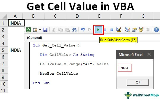
Be it Excel or VBA, we all need to work with cells because it will store all the data in cells. So, it all boils down to how well we know about cells in VBA. So, if cells are such a crucial part of the VBA, then it is important to understand them well. So, if you are a starter regarding VBA cells, this article will guide you on how to get cell values in Excel VBA in detail.
First, we can reference or work with cells in VBA in two ways: using CELLS propertyCells are cells of the worksheet, and in VBA, when we refer to cells as a range property, we refer to the same cells. In VBA concepts, cells are also the same, no different from normal excel cells.read more and RANGE object. Of course, why CELLS is a property and why RANGE is an object is a different analogy. Later in the article, we will get to that point.
Table of contents
- Get Cell Value with Excel VBA
- Examples of getting Cell Value in Excel VBA
- Example #1 – Using RANGE or CELLS Property
- Example #2 – Get Value from Cell in Excel VBA
- Example #3 – Get Value from One Cell to Another Cell
- Things to Remember
- Recommended Articles
- Examples of getting Cell Value in Excel VBA
You are free to use this image on your website, templates, etc, Please provide us with an attribution linkArticle Link to be Hyperlinked
For eg:
Source: Get Cell Value in Excel VBA (wallstreetmojo.com)
Examples of getting Cell Value in Excel VBA
Below are the examples of getting cell values in Excel VBA.
You can download this VBA Get Cell Value Excel Template here – VBA Get Cell Value Excel Template
Example #1 – Using RANGE or CELLS Property
In cell A1 we have a value of “India.”

We can reference this cell with a CELLS property or RANGE object. Let us see both of them in detail.
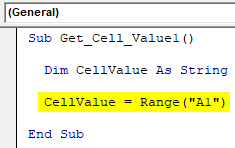
Using Range Property
First, start the macro procedure.
Code:
Sub Get_Cell_Value()

End Sub

Now open the RANGE object.
Code:
Sub Get_Cell_Value()

Range(

End Sub

The first argument of this object is “Cell1,” which is the cell we are referring to. In this case, it is cell A1, so we need to supply the cell address in double quotes for the RANGE object.
Code:
Sub Get_Cell_Value()

Range("A1")

End Sub

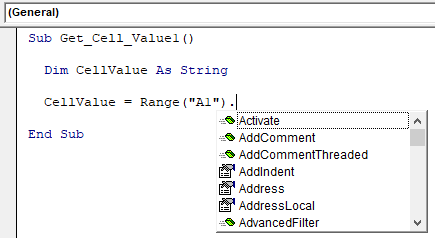
Since only one cell refers to other parameters is irrelevant, close the bracket and put a dot to see the IntelliSense list.

As you can see above, the moment we put a dot, we can see all the available IntelliSense lists of properties and methods of range objects.
Since we are selecting the cell, we need to choose the “SELECT” method from the IntelliSense list.
Code:
Sub Get_Cell_Value()

Range("A1").Select

End Sub

Now, select the cell other than A1 and run the code.
It does not matter which cell you select when you run the code. It has chosen the mentioned cell, i.e., the A1 cell.
Using Cells Property
Similarly, we use the CELLS property now.
Code:
Sub Get_Cell_Value()

Range("A1").Select
Cells(

End Sub

Unlike the RANGE object, we could directly supply the cell address. However, using this CELLS property, we cannot do that.
The first argument of this property is “Row Index,” i.e., which row we are referring to. Since we are selecting cell A1 we are referring to the first row, so mention 1.

The next argument is the “Column Index,” i.e., which column we refer to. For example, the A1 cell column is the first column, so enter 1.

Our code reads CELLS (1, 1) i.e. first row first column = A1.
Now, put a dot and see whether you get to see the IntelliSense list or not.

We cannot see any IntelliSense list with CELLS properties, so we must be sure what we are writing. Enter “Select” as the method.
Code:
Sub Get_Cell_Value()

Range("A1").Select
Cells(1, 1).Select

End Sub

This will also select cell A1.
Example #2 – Get Value from Cell in Excel VBA
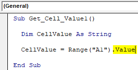
Selecting is the first thing we have learned. Now, we will see how to get value from cells. Before we select the cell, we need to define the variable to store the value from the cell.
Code:
Sub Get_Cell_Value1()

Dim CellValue As String

End Sub

Now, mention the cell address using either the RANGE object or the CELLS property. Since you are a beginner, use the RANGE object only because we can see the IntelliSense list with the RANGE object.
For the defined variable, put an equal sign and mention the cell address.
Code:
Sub Get_Cell_Value1()

Dim CellValue As String

CellValue = Range("A1")

End Sub
Once again, put a dot to see the IntelliSense list.
From the VBA IntelliSense list, choose the “Value” property to get the value from the mentioned cell.
Code:
Sub Get_Cell_Value1()

Dim CellValue As String

CellValue = Range("A1").Value

End Sub
Now, the variable “CellValue” holds the value from cell A1. Show this variable value in the message box in VBA.
Code:
Sub Get_Cell_Value1()

Dim CellValue As String

CellValue = Range("A1").Value

MsgBox CellValue

End Sub

Run the code and see the result in a message box.
Since there is a value of “INDIA” in cell A1, the same thing also appeared in the message box. Like this, we can get the value of the cell by the VBA valueIn VBA, the value property is usually used alongside the range method to assign a value to a range. It’s a VBA built-in expression that we can use with other functions.read more of the cell.
Example #3 – Get Value from One Cell to Another Cell
We know how to get value from the cell using VBA. Now, the question is how to insert a value into the cell. Let us take the same example only. For cell A1, we need to insert the value of “INDIA,” which we can do from the code below.
Code:
Sub Get_Cell_Value2()

Range("A1").Value = "INDIA"

End Sub

It will insert the value of “INDIA” to cell A1. Similarly, we can write the code below to get value from one cell to another.
Code:
Sub Get_Cell_Value2()

Range("A5").Value = Range("A1").Value

End Sub

Let me explain the code to you.
For cell A5, we need the value from the cell A1 value; that’s all this code says. So, this will get the value from cell A1 to A5 using VBA codeVBA code refers to a set of instructions written by the user in the Visual Basic Applications programming language on a Visual Basic Editor (VBE) to perform a specific task.read more.

Things to Remember
- Inserting value to cells and getting value from the cell requires the VBA “VALUE” property to be used.
- We can select only one cell using the CELLS property but use the RANGE object. Likewise, we can select multiple cells.
Recommended Articles
This article has been a guide to Get Cell Value in Excel VBA. Here, we discuss the examples of getting cell values using a range of cell properties in Excel VBA and a downloadable Excel template. Below you can find some useful Excel VBA articles: –
- VBA Variable Range
- Split String into Array in VBA
- Range Cells in VBA
- Active Cell in VBA