
Excel for Microsoft 365 Excel 2021 Excel 2019 Excel 2016 Excel 2013 Excel 2010 More…Less
Excel is an incredibly powerful tool for getting meaning out of vast amounts of data. But it also works really well for simple calculations and tracking almost any kind of information. The key for unlocking all that potential is the grid of cells. Cells can contain numbers, text, or formulas. You put data in your cells and group them in rows and columns. That allows you to add up your data, sort and filter it, put it in tables, and build great-looking charts. Let’s go through the basic steps to get you started.
Excel documents are called workbooks. Each workbook has sheets, typically called spreadsheets. You can add as many sheets as you want to a workbook, or you can create new workbooks to keep your data separate.
-
Click File, and then click New.
-
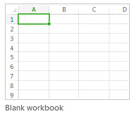
Under New, click the Blank workbook.

-
Click an empty cell.
For example, cell A1 on a new sheet. Cells are referenced by their location in the row and column on the sheet, so cell A1 is in the first row of column A.
-
Type text or a number in the cell.
-
Press Enter or Tab to move to the next cell.
-
Select the cell or range of cells that you want to add a border to.
-
On the Home tab, in the Font group, click the arrow next to Borders, and then click the border style that you want.
For more information, see Apply or remove cell borders on a worksheet .
-
Select the cell or range of cells that you want to apply cell shading to.
-
On the Home tab, in the Font group, choose the arrow next to Fill Color
, and then under Theme Colors or Standard Colors, select the color that you want.
 , and then under Theme Colors or Standard Colors, select the color that you want.
For more information about how to apply formatting to a worksheet, see Format a worksheet.
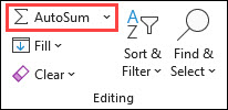
When you’ve entered numbers in your sheet, you might want to add them up. A fast way to do that is by using AutoSum.
-
Select the cell to the right or below the numbers you want to add.
-
Click the Home tab, and then click AutoSum in the Editing group.
AutoSum adds up the numbers and shows the result in the cell you selected.
For more information, see Use AutoSum to sum numbers
Adding numbers is just one of the things you can do, but Excel can do other math as well. Try some simple formulas to add, subtract, multiply, or divide your numbers.
-
Pick a cell, and then type an equal sign (=).
That tells Excel that this cell will contain a formula.
-
Type a combination of numbers and calculation operators, like the plus sign (+) for addition, the minus sign (-) for subtraction, the asterisk (*) for multiplication, or the forward slash (/) for division.
For example, enter =2+4, =4-2, =2*4, or =4/2.
-
Press Enter.
This runs the calculation.
You can also press Ctrl+Enter if you want the cursor to stay on the active cell.
For more information, see Create a simple formula.
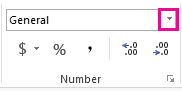
To distinguish between different types of numbers, add a format, like currency, percentages, or dates.
-
Select the cells that have numbers you want to format.
-
Click the Home tab, and then click the arrow in the General box.
-
Pick a number format.
If you don’t see the number format you’re looking for, click More Number Formats. For more information, see Available number formats.

A simple way to access Excel’s power is to put your data in a table. That lets you quickly filter or sort your data.
-
Select your data by clicking the first cell and dragging to the last cell in your data.
To use the keyboard, hold down Shift while you press the arrow keys to select your data.
-
Click the Quick Analysis button
in the bottom-right corner of the selection.
-
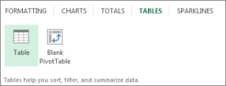
Click Tables, move your cursor to the Table button to preview your data, and then click the Table button.
-
Click the arrow
in the table header of a column. -
To filter the data, clear the Select All check box, and then select the data you want to show in your table.
-
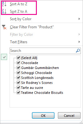
To sort the data, click Sort A to Z or Sort Z to A.
-
Click OK.
 in the bottom-right corner of the selection.
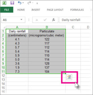
 in the table header of a column.
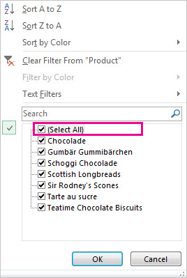
For more information, see Create or delete an Excel table
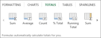
The Quick Analysis tool (available in Excel 2016 and Excel 2013 only) let you total your numbers quickly. Whether it’s a sum, average, or count you want, Excel shows the calculation results right below or next to your numbers.
-
Select the cells that contain numbers you want to add or count.
-
Click the Quick Analysis button
in the bottom-right corner of the selection. -
Click Totals, move your cursor across the buttons to see the calculation results for your data, and then click the button to apply the totals.
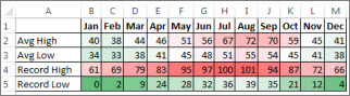
Conditional formatting or sparklines can highlight your most important data or show data trends. Use the Quick Analysis tool (available in Excel 2016 and Excel 2013 only) for a Live Preview to try it out.
-
Select the data you want to examine more closely.
-
Click the Quick Analysis button
in the bottom-right corner of the selection. -
Explore the options on the Formatting and Sparklines tabs to see how they affect your data.
For example, pick a color scale in the Formatting gallery to differentiate high, medium, and low temperatures.
-
When you like what you see, click that option.
 in the bottom-right corner of the selection.
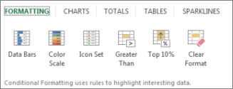
Learn more about how to analyze trends in data using sparklines.
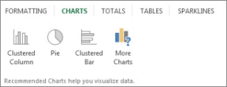
The Quick Analysis tool (available in Excel 2016 and Excel 2013 only) recommends the right chart for your data and gives you a visual presentation in just a few clicks.
-
Select the cells that contain the data you want to show in a chart.
-
Click the Quick Analysis button
in the bottom-right corner of the selection. -
Click the Charts tab, move across the recommended charts to see which one looks best for your data, and then click the one that you want.
Note: Excel shows different charts in this gallery, depending on what’s recommended for your data.
Learn about other ways to create a chart.
To quickly sort your data
-
Select a range of data, such as A1:L5 (multiple rows and columns) or C1:C80 (a single column). The range can include titles that you created to identify columns or rows.
-
Select a single cell in the column on which you want to sort.
-
Click
to perform an ascending sort (A to Z or smallest number to largest). -
Click
to perform a descending sort (Z to A or largest number to smallest).
 to perform an ascending sort (A to Z or smallest number to largest).
 to perform a descending sort (Z to A or largest number to smallest).
To sort by specific criteria
-
Select a single cell anywhere in the range that you want to sort.
-
On the Data tab, in the Sort & Filter group, choose Sort.
-
The Sort dialog box appears.
-
In the Sort by list, select the first column on which you want to sort.
-
In the Sort On list, select either Values, Cell Color, Font Color, or Cell Icon.
-
In the Order list, select the order that you want to apply to the sort operation — alphabetically or numerically ascending or descending (that is, A to Z or Z to A for text or lower to higher or higher to lower for numbers).
For more information about how to sort data, see Sort data in a range or table .
-
Select the data that you want to filter.
-
On the Data tab, in the Sort & Filter group, click Filter.
-
Click the arrow
in the column header to display a list in which you can make filter choices. -
To select by values, in the list, clear the (Select All) check box. This removes the check marks from all the check boxes. Then, select only the values you want to see, and click OK to see the results.
For more information about how to filter data, see Filter data in a range or table.
-
Click the Save button on the Quick Access Toolbar, or press Ctrl+S.
If you’ve saved your work before, you’re done.
-
If this is the first time you’ve save this file:
-
Under Save As, pick where to save your workbook, and then browse to a folder.
-
In the File name box, enter a name for your workbook.
-
Click Save.
-

-
Click File, and then click Print, or press Ctrl+P.
-
Preview the pages by clicking the Next Page and Previous Page arrows.
The preview window displays the pages in black and white or in color, depending on your printer settings.
If you don’t like how your pages will be printed, you can change page margins or add page breaks.
-
Click Print.

-
On the File tab, choose Options, and then choose the Add-Ins category.
-
Near the bottom of the Excel Options dialog box, make sure that Excel Add-ins is selected in the Manage box, and then click Go.
-
In the Add-Ins dialog box, select the check boxes the add-ins that you want to use, and then click OK.
If Excel displays a message that states it can’t run this add-in and prompts you to install it, click Yes to install the add-ins.
For more information about how to use add-ins, see Add or remove add-ins.
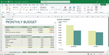
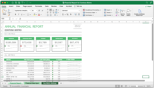
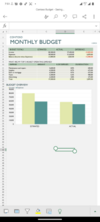
Excel allows you to apply built-in templates, to apply your own custom templates, and to search from a variety of templates on Office.com. Office.com provides a wide selection of popular Excel templates, including budgets.
For more information about how to find and apply templates, see Download free, pre-built templates.
Need more help?
Microsoft Excel is a spreadsheet developed by Microsoft for Windows, macOS, Android, iOS and iPadOS. It features calculation or computation capabilities, graphing tools, pivot tables, and a macro programming language called Visual Basic for Applications (VBA). Excel forms part of the Microsoft 365 suite of software.
 |
|
A simple bar graph being created in Excel, running on Windows 11 |
|
| Developer(s) | Microsoft |
|---|---|
| Initial release | November 19, 1987; 35 years ago |
| Stable release |
2103 (16.0.13901.20400) |
| Written in | C++ (back-end)[2] |
| Operating system | Microsoft Windows |
| Type | Spreadsheet |
| License | Trialware[3] |
| Website | microsoft.com/en-us/microsoft-365/excel |
Excel for Mac (version 16.67), running on macOS Big Sur 11.5.2 |
|
| Developer(s) | Microsoft |
|---|---|
| Initial release | September 30, 1985; 37 years ago |
| Stable release |
16.70 (Build 23021201) |
| Written in | C++ (back-end), Objective-C (API/UI)[2] |
| Operating system | macOS |
| Type | Spreadsheet |
| License | Proprietary commercial software |
| Website | products.office.com/mac |
Excel for Android running on Android 13 |
|
| Developer(s) | Microsoft Corporation |
|---|---|
| Stable release |
16.0.14729.20146 |
| Operating system | Android Oreo and later |
| Type | Spreadsheet |
| License | Proprietary commercial software |
| Website | products.office.com/en-us/excel |
| Developer(s) | Microsoft Corporation |
|---|---|
| Stable release |
2.70.1 |
| Operating system | iOS 15 or later iPadOS 15 or later |
| Type | Spreadsheet |
| License | Proprietary commercial software |
| Website | products.office.com/en-us/excel |
Features
Basic operation
Microsoft Excel has the basic features of all spreadsheets,[7] using a grid of cells arranged in numbered rows and letter-named columns to organize data manipulations like arithmetic operations. It has a battery of supplied functions to answer statistical, engineering, and financial needs. In addition, it can display data as line graphs, histograms and charts, and with a very limited three-dimensional graphical display. It allows sectioning of data to view its dependencies on various factors for different perspectives (using pivot tables and the scenario manager).[8] A PivotTable is a tool for data analysis. It does this by simplifying large data sets via PivotTable fields. It has a programming aspect, Visual Basic for Applications, allowing the user to employ a wide variety of numerical methods, for example, for solving differential equations of mathematical physics,[9][10] and then reporting the results back to the spreadsheet. It also has a variety of interactive features allowing user interfaces that can completely hide the spreadsheet from the user, so the spreadsheet presents itself as a so-called application, or decision support system (DSS), via a custom-designed user interface, for example, a stock analyzer,[11] or in general, as a design tool that asks the user questions and provides answers and reports.[12][13] In a more elaborate realization, an Excel application can automatically poll external databases and measuring instruments using an update schedule,[14] analyze the results, make a Word report or PowerPoint slide show, and e-mail these presentations on a regular basis to a list of participants. Excel was not designed to be used as a database.[citation needed]
Microsoft allows for a number of optional command-line switches to control the manner in which Excel starts.[15]
Functions
Excel 2016 has 484 functions.[16] Of these, 360 existed prior to Excel 2010. Microsoft classifies these functions in 14 categories. Of the 484 current functions, 386 may be called from VBA as methods of the object «WorksheetFunction»[17] and 44 have the same names as VBA functions.[18]
With the introduction of LAMBDA, Excel will become Turing complete.[19]
Macro programming
VBA programming
Use of a user-defined function sq(x) in Microsoft Excel. The named variables x & y are identified in the Name Manager. The function sq is introduced using the Visual Basic editor supplied with Excel.
Subroutine in Excel calculates the square of named column variable x read from the spreadsheet, and writes it into the named column variable y.
The Windows version of Excel supports programming through Microsoft’s Visual Basic for Applications (VBA), which is a dialect of Visual Basic. Programming with VBA allows spreadsheet manipulation that is awkward or impossible with standard spreadsheet techniques. Programmers may write code directly using the Visual Basic Editor (VBE), which includes a window for writing code, debugging code, and code module organization environment. The user can implement numerical methods as well as automating tasks such as formatting or data organization in VBA[20] and guide the calculation using any desired intermediate results reported back to the spreadsheet.
VBA was removed from Mac Excel 2008, as the developers did not believe that a timely release would allow porting the VBA engine natively to Mac OS X. VBA was restored in the next version, Mac Excel 2011,[21] although the build lacks support for ActiveX objects, impacting some high level developer tools.[22]
A common and easy way to generate VBA code is by using the Macro Recorder.[23] The Macro Recorder records actions of the user and generates VBA code in the form of a macro. These actions can then be repeated automatically by running the macro. The macros can also be linked to different trigger types like keyboard shortcuts, a command button or a graphic. The actions in the macro can be executed from these trigger types or from the generic toolbar options. The VBA code of the macro can also be edited in the VBE. Certain features such as loop functions and screen prompt by their own properties, and some graphical display items, cannot be recorded but must be entered into the VBA module directly by the programmer. Advanced users can employ user prompts to create an interactive program, or react to events such as sheets being loaded or changed.
Macro Recorded code may not be compatible with Excel versions. Some code that is used in Excel 2010 cannot be used in Excel 2003. Making a Macro that changes the cell colors and making changes to other aspects of cells may not be backward compatible.
VBA code interacts with the spreadsheet through the Excel Object Model,[24] a vocabulary identifying spreadsheet objects, and a set of supplied functions or methods that enable reading and writing to the spreadsheet and interaction with its users (for example, through custom toolbars or command bars and message boxes). User-created VBA subroutines execute these actions and operate like macros generated using the macro recorder, but are more flexible and efficient.
History
From its first version Excel supported end-user programming of macros (automation of repetitive tasks) and user-defined functions (extension of Excel’s built-in function library). In early versions of Excel, these programs were written in a macro language whose statements had formula syntax and resided in the cells of special-purpose macro sheets (stored with file extension .XLM in Windows.) XLM was the default macro language for Excel through Excel 4.0.[25] Beginning with version 5.0 Excel recorded macros in VBA by default but with version 5.0 XLM recording was still allowed as an option. After version 5.0 that option was discontinued. All versions of Excel, including Excel 2021 are capable of running an XLM macro, though Microsoft discourages their use.[26]
Charts
Graph made using Microsoft Excel
Excel supports charts, graphs, or histograms generated from specified groups of cells. It also supports Pivot Charts that allow for a chart to be linked directly to a Pivot table. This allows the chart to be refreshed with the Pivot Table. The generated graphic component can either be embedded within the current sheet or added as a separate object.
These displays are dynamically updated if the content of cells changes. For example, suppose that the important design requirements are displayed visually; then, in response to a user’s change in trial values for parameters, the curves describing the design change shape, and their points of intersection shift, assisting the selection of the best design.
Add-ins
Additional features are available using add-ins. Several are provided with Excel, including:
- Analysis ToolPak: Provides data analysis tools for statistical and engineering analysis (includes analysis of variance and regression analysis)
- Analysis ToolPak VBA: VBA functions for Analysis ToolPak
- Euro Currency Tools: Conversion and formatting for euro currency
- Solver Add-In: Tools for optimization and equation solving
Data storage and communication
Number of rows and columns
Versions of Excel up to 7.0 had a limitation in the size of their data sets of 16K (214 = 16384) rows. Versions 8.0 through 11.0 could handle 64K (216 = 65536) rows and 256 columns (28 as label ‘IV’). Version 12.0 onwards, including the current Version 16.x, can handle over 1M (220 = 1048576) rows, and 16384 (214, labeled as column ‘XFD’) columns.[27]
File formats
| Filename extension |
.xls, (.xlsx, .xlsm, .xlsb — Excel 2007) |
|---|---|
| Internet media type |
application/vnd.ms-excel |
| Uniform Type Identifier (UTI) | com.microsoft.excel.xls |
| Developed by | Microsoft |
| Type of format | Spreadsheet |
Microsoft Excel up until 2007 version used a proprietary binary file format called Excel Binary File Format (.XLS) as its primary format.[28] Excel 2007 uses Office Open XML as its primary file format, an XML-based format that followed after a previous XML-based format called «XML Spreadsheet» («XMLSS»), first introduced in Excel 2002.[29]
Although supporting and encouraging the use of new XML-based formats as replacements, Excel 2007 remained backwards-compatible with the traditional, binary formats. In addition, most versions of Microsoft Excel can read CSV, DBF, SYLK, DIF, and other legacy formats. Support for some older file formats was removed in Excel 2007.[30] The file formats were mainly from DOS-based programs.
Binary
OpenOffice.org has created documentation of the Excel format. Two epochs of the format exist: the 97-2003 OLE format, and the older stream format.[31] Microsoft has made the Excel binary format specification available to freely download.[32]
XML Spreadsheet
The XML Spreadsheet format introduced in Excel 2002[29] is a simple, XML based format missing some more advanced features like storage of VBA macros. Though the intended file extension for this format is .xml, the program also correctly handles XML files with .xls extension. This feature is widely used by third-party applications (e.g. MySQL Query Browser) to offer «export to Excel» capabilities without implementing binary file format. The following example will be correctly opened by Excel if saved either as Book1.xml or Book1.xls:
<?xml version="1.0"?>
<Workbook xmlns="urn:schemas-microsoft-com:office:spreadsheet"
 xmlns:o="urn:schemas-microsoft-com:office:office"
 xmlns:x="urn:schemas-microsoft-com:office:excel"
 xmlns:ss="urn:schemas-microsoft-com:office:spreadsheet"
 xmlns:html="http://www.w3.org/TR/REC-html40">
 <Worksheet ss:Name="Sheet1">
  <Table ss:ExpandedColumnCount="2" ss:ExpandedRowCount="2" x:FullColumns="1" x:FullRows="1">
   <Row>
    <Cell><Data ss:Type="String">Name</Data></Cell>
    <Cell><Data ss:Type="String">Example</Data></Cell>
   </Row>
   <Row>
    <Cell><Data ss:Type="String">Value</Data></Cell>
    <Cell><Data ss:Type="Number">123</Data></Cell>
   </Row>
  </Table>
 </Worksheet>
</Workbook>
Current file extensions
Microsoft Excel 2007, along with the other products in the Microsoft Office 2007 suite, introduced new file formats. The first of these (.xlsx) is defined in the Office Open XML (OOXML) specification.
| Format | Extension | Description |
|---|---|---|
| Excel Workbook | .xlsx
|
The default Excel 2007 and later workbook format. In reality, a ZIP compressed archive with a directory structure of XML text documents. Functions as the primary replacement for the former binary .xls format, although it does not support Excel macros for security reasons. Saving as .xlsx offers file size reduction over .xls[33] |
| Excel Macro-enabled Workbook | .xlsm
|
As Excel Workbook, but with macro support. |
| Excel Binary Workbook | .xlsb
|
As Excel Macro-enabled Workbook, but storing information in binary form rather than XML documents for opening and saving documents more quickly and efficiently. Intended especially for very large documents with tens of thousands of rows, and/or several hundreds of columns. This format is very useful for shrinking large Excel files as is often the case when doing data analysis. |
| Excel Macro-enabled Template | .xltm
|
A template document that forms a basis for actual workbooks, with macro support. The replacement for the old .xlt format. |
| Excel Add-in | .xlam
|
Excel add-in to add extra functionality and tools. Inherent macro support because of the file purpose. |
Old file extensions
| Format | Extension | Description |
|---|---|---|
| Spreadsheet | .xls
|
Main spreadsheet format which holds data in worksheets, charts, and macros |
| Add-in (VBA) | .xla
|
Adds custom functionality; written in VBA |
| Toolbar | .xlb
|
The file extension where Microsoft Excel custom toolbar settings are stored. |
| Chart | .xlc
|
A chart created with data from a Microsoft Excel spreadsheet that only saves the chart. To save the chart and spreadsheet save as .XLS. XLC is not supported in Excel 2007 or in any newer versions of Excel. |
| Dialog | .xld
|
Used in older versions of Excel. |
| Archive | .xlk
|
A backup of an Excel Spreadsheet |
| Add-in (DLL) | .xll
|
Adds custom functionality; written in C++/C, Fortran, etc. and compiled in to a special dynamic-link library |
| Macro | .xlm
|
A macro is created by the user or pre-installed with Excel. |
| Template | .xlt
|
A pre-formatted spreadsheet created by the user or by Microsoft Excel. |
| Module | .xlv
|
A module is written in VBA (Visual Basic for Applications) for Microsoft Excel |
| Library | .DLL
|
Code written in VBA may access functions in a DLL, typically this is used to access the Windows API |
| Workspace | .xlw
|
Arrangement of the windows of multiple Workbooks |
Using other Windows applications
Windows applications such as Microsoft Access and Microsoft Word, as well as Excel can communicate with each other and use each other’s capabilities. The most common are Dynamic Data Exchange: although strongly deprecated by Microsoft, this is a common method to send data between applications running on Windows, with official MS publications referring to it as «the protocol from hell».[34] As the name suggests, it allows applications to supply data to others for calculation and display. It is very common in financial markets, being used to connect to important financial data services such as Bloomberg and Reuters.
OLE Object Linking and Embedding allows a Windows application to control another to enable it to format or calculate data. This may take on the form of «embedding» where an application uses another to handle a task that it is more suited to, for example a PowerPoint presentation may be embedded in an Excel spreadsheet or vice versa.[35][36][37][38]
Using external data
Excel users can access external data sources via Microsoft Office features such as (for example) .odc connections built with the Office Data Connection file format. Excel files themselves may be updated using a Microsoft supplied ODBC driver.
Excel can accept data in real-time through several programming interfaces, which allow it to communicate with many data sources such as Bloomberg and Reuters (through addins such as Power Plus Pro).
- DDE: «Dynamic Data Exchange» uses the message passing mechanism in Windows to allow data to flow between Excel and other applications. Although it is easy for users to create such links, programming such links reliably is so difficult that Microsoft, the creators of the system, officially refer to it as «the protocol from hell».[34] In spite of its many issues DDE remains the most common way for data to reach traders in financial markets.
- Network DDE Extended the protocol to allow spreadsheets on different computers to exchange data. Starting with Windows Vista, Microsoft no longer supports the facility.[39]
- Real Time Data: RTD although in many ways technically superior to DDE, has been slow to gain acceptance, since it requires non-trivial programming skills, and when first released was neither adequately documented nor supported by the major data vendors.[40][41]
Alternatively, Microsoft Query provides ODBC-based browsing within Microsoft Excel.[42][43][44]
Export and migration of spreadsheets
Programmers have produced APIs to open Excel spreadsheets in a variety of applications and environments other than Microsoft Excel. These include opening Excel documents on the web using either ActiveX controls, or plugins like the Adobe Flash Player. The Apache POI opensource project provides Java libraries for reading and writing Excel spreadsheet files.
Password protection
Microsoft Excel protection offers several types of passwords:
- Password to open a document[45]
- Password to modify a document[46]
- Password to unprotect the worksheet
- Password to protect workbook
- Password to protect the sharing workbook[47]
All passwords except password to open a document can be removed instantly regardless of the Microsoft Excel version used to create the document. These types of passwords are used primarily for shared work on a document. Such password-protected documents are not encrypted, and a data sources from a set password is saved in a document’s header. Password to protect workbook is an exception – when it is set, a document is encrypted with the standard password «VelvetSweatshop», but since it is known to the public, it actually does not add any extra protection to the document. The only type of password that can prevent a trespasser from gaining access to a document is password to open a document. The cryptographic strength of this kind of protection depends strongly on the Microsoft Excel version that was used to create the document.
In Microsoft Excel 95 and earlier versions, the password to open is converted to a 16-bit key that can be instantly cracked. In Excel 97/2000 the password is converted to a 40-bit key, which can also be cracked very quickly using modern equipment. As regards services that use rainbow tables (e.g. Password-Find), it takes up to several seconds to remove protection. In addition, password-cracking programs can brute-force attack passwords at a rate of hundreds of thousands of passwords a second, which not only lets them decrypt a document but also find the original password.
In Excel 2003/XP the encryption is slightly better – a user can choose any encryption algorithm that is available in the system (see Cryptographic Service Provider). Due to the CSP, an Excel file cannot be decrypted, and thus the password to open cannot be removed, though the brute-force attack speed remains quite high. Nevertheless, the older Excel 97/2000 algorithm is set by the default. Therefore, users who do not change the default settings lack reliable protection of their documents.
The situation changed fundamentally in Excel 2007, where the modern AES algorithm with a key of 128 bits started being used for decryption, and a 50,000-fold use of the hash function SHA1 reduced the speed of brute-force attacks down to hundreds of passwords per second. In Excel 2010, the strength of the protection by the default was increased two times due to the use of a 100,000-fold SHA1 to convert a password to a key.
Other platforms
Excel for mobile
Excel Mobile is a spreadsheet program that can edit XLSX files. It can edit and format text in cells, calculate formulas, search within the spreadsheet, sort rows and columns, freeze panes, filter the columns, add comments, and create charts. It cannot add columns or rows except at the edge of the document, rearrange columns or rows, delete rows or columns, or add spreadsheet tabs.[48][49][50][51][52][53] The 2007 version has the ability to use a full-screen mode to deal with limited screen resolution, as well as split panes to view different parts of a worksheet at one time.[51] Protection settings, zoom settings, autofilter settings, certain chart formatting, hidden sheets, and other features are not supported on Excel Mobile, and will be modified upon opening and saving a workbook.[52] In 2015, Excel Mobile became available for Windows 10 and Windows 10 Mobile on Windows Store.[54][55]
Excel for the web
Excel for the web is a free lightweight version of Microsoft Excel available as part of Office on the web, which also includes web versions of Microsoft Word and Microsoft PowerPoint.
Excel for the web can display most of the features available in the desktop versions of Excel, although it may not be able to insert or edit them. Certain data connections are not accessible on Excel for the web, including with charts that may use these external connections. Excel for the web also cannot display legacy features, such as Excel 4.0 macros or Excel 5.0 dialog sheets. There are also small differences between how some of the Excel functions work.[56]
Microsoft Excel Viewer
Microsoft Excel Viewer was a freeware program for Microsoft Windows for viewing and printing spreadsheet documents created by Excel.[57] Microsoft retired the viewer in April 2018 with the last security update released in February 2019 for Excel Viewer 2007 (SP3).[58][59]
The first version released by Microsoft was Excel 97 Viewer.[60][61] Excel 97 Viewer was supported in Windows CE for Handheld PCs.[62] In October 2004, Microsoft released Excel Viewer 2003.[63] In September 2007, Microsoft released Excel Viewer 2003 Service Pack 3 (SP3).[64] In January 2008, Microsoft released Excel Viewer 2007 (featuring a non-collapsible Ribbon interface).[65] In April 2009, Microsoft released Excel Viewer 2007 Service Pack 2 (SP2).[66] In October 2011, Microsoft released Excel Viewer 2007 Service Pack 3 (SP3).[67]
Microsoft advises to view and print Excel files for free to use the Excel Mobile application for Windows 10 and for Windows 7 and Windows 8 to upload the file to OneDrive and use Excel for the web with a Microsoft account to open them in a browser.[58][68]
Quirks
In addition to issues with spreadsheets in general, other problems specific to Excel include numeric precision, misleading statistics functions, mod function errors, date limitations and more.
Numeric precision
Excel maintains 15 figures in its numbers, but they are not always accurate: the bottom line should be the same as the top line.
Despite the use of 15-figure precision, Excel can display many more figures (up to thirty) upon user request. But the displayed figures are not those actually used in its computations, and so, for example, the difference of two numbers may differ from the difference of their displayed values. Although such departures are usually beyond the 15th decimal, exceptions do occur, especially for very large or very small numbers. Serious errors can occur if decisions are made based upon automated comparisons of numbers (for example, using the Excel If function), as equality of two numbers can be unpredictable.[citation needed]
In the figure, the fraction 1/9000 is displayed in Excel. Although this number has a decimal representation that is an infinite string of ones, Excel displays only the leading 15 figures. In the second line, the number one is added to the fraction, and again Excel displays only 15 figures. In the third line, one is subtracted from the sum using Excel. Because the sum in the second line has only eleven 1’s after the decimal, the difference when 1 is subtracted from this displayed value is three 0’s followed by a string of eleven 1’s. However, the difference reported by Excel in the third line is three 0’s followed by a string of thirteen 1’s and two extra erroneous digits. This is because Excel calculates with about half a digit more than it displays.
Excel works with a modified 1985 version of the IEEE 754 specification.[69] Excel’s implementation involves conversions between binary and decimal representations, leading to accuracy that is on average better than one would expect from simple fifteen digit precision, but that can be worse. See the main article for details.
Besides accuracy in user computations, the question of accuracy in Excel-provided functions may be raised. Particularly in the arena of statistical functions, Excel has been criticized for sacrificing accuracy for speed of calculation.[70][71]
As many calculations in Excel are executed using VBA, an additional issue is the accuracy of VBA, which varies with variable type and user-requested precision.[72]
Statistical functions
The accuracy and convenience of statistical tools in Excel has been criticized,[73][74][75][76][77] as mishandling missing data, as returning incorrect values due to inept handling of round-off and large numbers, as only selectively updating calculations on a spreadsheet when some cell values are changed, and as having a limited set of statistical tools. Microsoft has announced some of these issues are addressed in Excel 2010.[78]
Excel MOD function error
Excel has issues with modulo operations. In the case of excessively large results, Excel will return the error warning #NUM! instead of an answer.[79]
Fictional leap day in the year 1900
Excel includes February 29, 1900, incorrectly treating 1900 as a leap year, even though e.g. 2100 is correctly treated as a non-leap year.[80][81] The bug originated from Lotus 1-2-3 (deliberately implemented to save computer memory), and was also purposely implemented in Excel, for the purpose of bug compatibility.[82] This legacy has later been carried over into Office Open XML file format.[83]
Thus a (not necessarily whole) number greater than or equal to 61 interpreted as a date and time are the (real) number of days after December 30, 1899, 0:00, a non-negative number less than 60 is the number of days after December 31, 1899, 0:00, and numbers with whole part 60 represent the fictional day.
Date range
Excel supports dates with years in the range 1900–9999, except that December 31, 1899, can be entered as 0 and is displayed as 0-jan-1900.
Converting a fraction of a day into hours, minutes and days by treating it as a moment on the day January 1, 1900, does not work for a negative fraction.[84]
Conversion problems
Entering text that happens to be in a form that is interpreted as a date, the text can be unintentionally changed to a standard date format. A similar problem occurs when a text happens to be in the form of a floating-point notation of a number. In these cases the original exact text cannot be recovered from the result. Formatting the cell as TEXT before entering ambiguous text prevents Excel from converting to a date.
This issue has caused a well known problem in the analysis of DNA, for example in bioinformatics. As first reported in 2004,[85] genetic scientists found that Excel automatically and incorrectly converts certain gene names into dates. A follow-up study in 2016 found many peer reviewed scientific journal papers had been affected and that «Of the selected journals, the proportion of published articles with Excel files containing gene lists that are affected by gene name errors is 19.6 %.»[86] Excel parses the copied and pasted data and sometimes changes them depending on what it thinks they are. For example, MARCH1 (Membrane Associated Ring-CH-type finger 1) gets converted to the date March 1 (1-Mar) and SEPT2 (Septin 2) is converted into September 2 (2-Sep) etc.[87] While some secondary news sources[88] reported this as a fault with Excel, the original authors of the 2016 paper placed the blame with the researchers misusing Excel.[86][89]
In August 2020 the HUGO Gene Nomenclature Committee (HGNC) published new guidelines in the journal Nature regarding gene naming in order to avoid issues with «symbols that affect data handling and retrieval.» So far 27 genes have been renamed, including changing MARCH1 to MARCHF1 and SEPT1 to SEPTIN1 in order to avoid accidental conversion of the gene names into dates.[90]
Errors with large strings
The following functions return incorrect results when passed a string longer than 255 characters:[91]
type()incorrectly returns 16, meaning «Error value»IsText(), when called as a method of the VBA objectWorksheetFunction(i.e.,WorksheetFunction.IsText()in VBA), incorrectly returns «false».
Filenames
Microsoft Excel will not open two documents with the same name and instead will display the following error:
- A document with the name ‘%s’ is already open. You cannot open two documents with the same name, even if the documents are in different folders. To open the second document, either close the document that is currently open, or rename one of the documents.[92]
The reason is for calculation ambiguity with linked cells. If there is a cell ='[Book1.xlsx]Sheet1'!$G$33, and there are two books named «Book1» open, there is no way to tell which one the user means.[93]
Versions
Early history
Microsoft originally marketed a spreadsheet program called Multiplan in 1982. Multiplan became very popular on CP/M systems, but on MS-DOS systems it lost popularity to Lotus 1-2-3. Microsoft released the first version of Excel for the Macintosh on September 30, 1985, and the first Windows version was 2.05 (to synchronize with the Macintosh version 2.2) on November 19, 1987.[94][95] Lotus was slow to bring 1-2-3 to Windows and by the early 1990s, Excel had started to outsell 1-2-3 and helped Microsoft achieve its position as a leading PC software developer. This accomplishment solidified Microsoft as a valid competitor and showed its future of developing GUI software. Microsoft maintained its advantage with regular new releases, every two years or so.
Microsoft Windows
Excel 2.0 is the first version of Excel for the Intel platform. Versions prior to 2.0 were only available on the Apple Macintosh.
Excel 2.0 (1987)
The first Windows version was labeled «2» to correspond to the Mac version. It was announced on October 6, 1987, and released on November 19.[96] This included a run-time version of Windows.[97]
BYTE in 1989 listed Excel for Windows as among the «Distinction» winners of the BYTE Awards. The magazine stated that the port of the «extraordinary» Macintosh version «shines», with a user interface as good as or better than the original.
Excel 3.0 (1990)
Included toolbars, drawing capabilities, outlining, add-in support, 3D charts, and many more new features.[97]
Excel 4.0 (1992)
Introduced auto-fill.[98]
Also, an easter egg in Excel 4.0 reveals a hidden animation of a dancing set of numbers 1 through 3, representing Lotus 1-2-3, which is then crushed by an Excel logo.[99]
Excel 5.0 (1993)
With version 5.0, Excel has included Visual Basic for Applications (VBA), a programming language based on Visual Basic which adds the ability to automate tasks in Excel and to provide user-defined functions (UDF) for use in worksheets. VBA includes a fully featured integrated development environment (IDE). Macro recording can produce VBA code replicating user actions, thus allowing simple automation of regular tasks. VBA allows the creation of forms and in‑worksheet controls to communicate with the user. The language supports use (but not creation) of ActiveX (COM) DLL’s; later versions add support for class modules allowing the use of basic object-oriented programming techniques.
The automation functionality provided by VBA made Excel a target for macro viruses. This caused serious problems until antivirus products began to detect these viruses. Microsoft belatedly took steps to prevent the misuse by adding the ability to disable macros completely, to enable macros when opening a workbook or to trust all macros signed using a trusted certificate.
Versions 5.0 to 9.0 of Excel contain various Easter eggs, including a «Hall of Tortured Souls», a Doom-like minigame, although since version 10 Microsoft has taken measures to eliminate such undocumented features from their products.[100]
5.0 was released in a 16-bit x86 version for Windows 3.1 and later in a 32-bit version for NT 3.51 (x86/Alpha/PowerPC)
Excel 95 (v7.0)
Released in 1995 with Microsoft Office for Windows 95, this is the first major version after Excel 5.0, as there is no Excel 6.0 with all of the Office applications standardizing on the same major version number.
Internal rewrite to 32-bits. Almost no external changes, but faster and more stable.
Excel 95 contained a hidden Doom-like mini-game called «The Hall of Tortured Souls», a series of rooms featuring the names and faces of the developers as an easter egg.[101]
Excel 97 (v8.0)
Included in Office 97 (for x86 and Alpha). This was a major upgrade that introduced the paper clip office assistant and featured standard VBA used instead of internal Excel Basic. It introduced the now-removed Natural Language labels.
This version of Excel includes a flight simulator as an Easter Egg.
Excel 2000 (v9.0)
Included in Office 2000. This was a minor upgrade but introduced an upgrade to the clipboard where it can hold multiple objects at once. The Office Assistant, whose frequent unsolicited appearance in Excel 97 had annoyed many users, became less intrusive.
A small 3-D game called «Dev Hunter» (inspired by Spy Hunter) was included as an easter egg.[102][103]
Excel 2002 (v10.0)
Included in Office XP. Very minor enhancements.
Excel 2003 (v11.0)
Included in Office 2003. Minor enhancements.
Excel 2007 (v12.0)
Included in Office 2007. This release was a major upgrade from the previous version. Similar to other updated Office products, Excel in 2007 used the new Ribbon menu system. This was different from what users were used to, and was met with mixed reactions. One study reported fairly good acceptance by users except highly experienced users and users of word processing applications with a classical WIMP interface, but was less convinced in terms of efficiency and organization.[104] However, an online survey reported that a majority of respondents had a negative opinion of the change, with advanced users being «somewhat more negative» than intermediate users, and users reporting a self-estimated reduction in productivity.
Added functionality included Tables,[105] and the SmartArt set of editable business diagrams. Also added was an improved management of named variables through the Name Manager, and much-improved flexibility in formatting graphs, which allow (x, y) coordinate labeling and lines of arbitrary weight. Several improvements to pivot tables were introduced.
Also like other office products, the Office Open XML file formats were introduced, including .xlsm for a workbook with macros and .xlsx for a workbook without macros.[106]
Specifically, many of the size limitations of previous versions were greatly increased. To illustrate, the number of rows was now 1,048,576 (220) and columns was 16,384 (214; the far-right column is XFD). This changes what is a valid A1 reference versus a named range. This version made more extensive use of multiple cores for the calculation of spreadsheets; however, VBA macros are not handled in parallel and XLL add‑ins were only executed in parallel if they were thread-safe and this was indicated at registration.
Excel 2010 (v14.0)
Microsoft Excel 2010 running on Windows 7
Included in Office 2010, this is the next major version after v12.0, as version number 13 was skipped.
Minor enhancements and 64-bit support,[107] including the following:
- Multi-threading recalculation (MTR) for commonly used functions
- Improved pivot tables
- More conditional formatting options
- Additional image editing capabilities
- In-cell charts called sparklines
- Ability to preview before pasting
- Office 2010 backstage feature for document-related tasks
- Ability to customize the Ribbon
- Many new formulas, most highly specialized to improve accuracy[108]
Excel 2013 (v15.0)
Included in Office 2013, along with a lot of new tools included in this release:
- Improved Multi-threading and Memory Contention
- FlashFill[109]
- Power View[110]
- Power Pivot[111]
- Timeline Slicer
- Windows App
- Inquire[112]
- 50 new functions[113]
Excel 2016 (v16.0)
Included in Office 2016, along with a lot of new tools included in this release:
- Power Query integration
- Read-only mode for Excel
- Keyboard access for Pivot Tables and Slicers in Excel
- New Chart Types
- Quick data linking in Visio
- Excel forecasting functions
- Support for multiselection of Slicer items using touch
- Time grouping and Pivot Chart Drill Down
- Excel data cards[114]
Excel 2019, Excel 2021, Office 365 and subsequent (v16.0)
Microsoft no longer releases Office or Excel in discrete versions. Instead, features are introduced automatically over time using Windows Update. The version number remains 16.0. Thereafter only the approximate dates when features appear can now be given.
- Dynamic Arrays. These are essentially Array Formulas but they «Spill» automatically into neighboring cells and does not need the ctrl-shift-enter to create them. Further, dynamic arrays are the default format, with new «@» and «#» operators to provide compatibility with previous versions. This is perhaps the biggest structural change since 2007, and is in response to a similar feature in Google Sheets. Dynamic arrays started appearing in pre-releases about 2018, and as of March 2020 are available in published versions of Office 365 provided a user selected «Office Insiders».
Apple Macintosh
Microsoft Excel for Mac 2011
- 1985 Excel 1.0
- 1988 Excel 1.5
- 1989 Excel 2.2
- 1990 Excel 3.0
- 1992 Excel 4.0
- 1993 Excel 5.0 (part of Office 4.x—Final Motorola 680×0 version[115] and first PowerPC version)
- 1998 Excel 8.0 (part of Office 98)
- 2000 Excel 9.0 (part of Office 2001)
- 2001 Excel 10.0 (part of Office v. X)
- 2004 Excel 11.0 (part of Office 2004)
- 2008 Excel 12.0 (part of Office 2008)
- 2010 Excel 14.0 (part of Office 2011)
- 2015 Excel 15.0 (part of Office 2016—Office 2016 for Mac brings the Mac version much closer to parity with its Windows cousin, harmonizing many of the reporting and high-level developer functions, while bringing the ribbon and styling into line with its PC counterpart.)[116]
OS/2
- 1989 Excel 2.2
- 1990 Excel 2.3
- 1991 Excel 3.0
Summary
| Legend: | Old version, not maintained | Older version, still maintained | Current stable version |
|---|
| Year | Name | Version | Comments |
|---|---|---|---|
| 1987 | Excel 2 | 2.0 | Renumbered to 2 to correspond with contemporary Macintosh version. Supported macros (later known as Excel 4 macros). |
| 1990 | Excel 3 | 3.0 | Added 3D graphing capabilities |
| 1992 | Excel 4 | 4.0 | Introduced auto-fill feature |
| 1993 | Excel 5 | 5.0 | Included Visual Basic for Applications (VBA) and various object-oriented options |
| 1995 | Excel 95 | 7.0 | Renumbered for contemporary Word version. Both programs were packaged in Microsoft Office by this time. |
| 1997 | Excel 97 | 8.0 | |
| 2000 | Excel 2000 | 9.0 | Part of Microsoft Office 2000, which was itself part of Windows Millennium (also known as «Windows ME»). |
| 2002 | Excel 2002 | 10.0 | |
| 2003 | Excel 2003 | 11.0 | Released only 1 year later to correspond better with the rest of Microsoft Office (Word, PowerPoint, etc.). |
| 2007 | Excel 2007 | 12.0 | |
| 2010 | Excel 2010 | 14.0 | Due to superstitions surrounding the number 13, Excel 13 was skipped in version counting. |
| 2013 | Excel 2013 | 15.0 | Introduced 50 more mathematical functions (available as pre-packaged commands, rather than typing the formula manually). |
| 2016 | Excel 2016 | 16.0 | Part of Microsoft Office 2016 |
| Year | Name | Version | Comments |
|---|---|---|---|
| 1985 | Excel 1 | 1.0 | Initial version of Excel. Supported macros (later known as Excel 4 macros). |
| 1988 | Excel 1.5 | 1.5 | |
| 1989 | Excel 2 | 2.2 | |
| 1990 | Excel 3 | 3.0 | |
| 1992 | Excel 4 | 4.0 | |
| 1993 | Excel 5 | 5.0 | Only available on PowerPC-based Macs. First PowerPC version. |
| 1998 | Excel 98 | 8.0 | Excel 6 and Excel 7 were skipped to correspond with the rest of Microsoft Office at the time. |
| 2000 | Excel 2000 | 9.0 | |
| 2001 | Excel 2001 | 10.0 | |
| 2004 | Excel 2004 | 11.0 | |
| 2008 | Excel 2008 | 12.0 | |
| 2011 | Excel 2011 | 14.0 | As with the Windows version, version 13 was skipped for superstitious reasons. |
| 2016 | Excel 2016 | 16.0 | As with the rest of Microsoft Office, so it is for Excel: Future release dates for the Macintosh version are intended to correspond better to those for the Windows version, from 2016 onward. |
| Year | Name | Version | Comments |
|---|---|---|---|
| 1989 | Excel 2.2 | 2.2 | Numbered in between Windows versions at the time |
| 1990 | Excel 2.3 | 2.3 | |
| 1991 | Excel 3 | 3.0 | Last OS/2 version. Discontinued subseries of Microsoft Excel, which is otherwise still an actively developed program. |
Impact
Excel offers many user interface tweaks over the earliest electronic spreadsheets; however, the essence remains the same as in the original spreadsheet software, VisiCalc: the program displays cells organized in rows and columns, and each cell may contain data or a formula, with relative or absolute references to other cells.
Excel 2.0 for Windows, which was modeled after its Mac GUI-based counterpart, indirectly expanded the installed base of the then-nascent Windows environment. Excel 2.0 was released a month before Windows 2.0, and the installed base of Windows was so low at that point in 1987 that Microsoft had to bundle a runtime version of Windows 1.0 with Excel 2.0.[117] Unlike Microsoft Word, there never was a DOS version of Excel.
Excel became the first spreadsheet to allow the user to define the appearance of spreadsheets (fonts, character attributes, and cell appearance). It also introduced intelligent cell re-computation, where only cells dependent on the cell being modified are updated (previous spreadsheet programs recomputed everything all the time or waited for a specific user command). Excel introduced auto-fill, the ability to drag and expand the selection box to automatically copy a cell or row contents to adjacent cells or rows, adjusting the copies intelligently by automatically incrementing cell references or contents. Excel also introduced extensive graphing capabilities.
Security
Because Excel is widely used, it has been attacked by hackers. While Excel is not directly exposed to the Internet, if an attacker can get a victim to open a file in Excel, and there is an appropriate security bug in Excel, then the attacker can gain control of the victim’s computer.[118] UK’s GCHQ has a tool named TORNADO ALLEY with this purpose.[119][120]
Games
Besides the easter eggs, numerous games have been created or recreated in Excel, such as Tetris, 2048, Scrabble, Yahtzee, Angry Birds, Pac-Man, Civilization, Monopoly, Battleship, Blackjack, Space Invaders, and others.[121][122][123][124][125]
In 2020, Excel became an esport with the advent of the Financial Modeling World Cup.[126]
See also
- Comparison of spreadsheet software
- Numbers (spreadsheet)—the iWork equivalent
- Spreadmart
- Financial Modeling World Cup, online esport financial modelling competition using Excel
References
- ^ «Update history for Microsoft Office 2019». Microsoft Docs. Retrieved April 13, 2021.
- ^ a b «C++ in MS Office». cppcon. July 17, 2014. Archived from the original on November 7, 2019. Retrieved June 25, 2019.
- ^ «Microsoft Office Excel 365». Microsoft.com. Retrieved January 25, 2021.
- ^ «Update history for Office for Mac». Microsoft Docs.
- ^ «Microsoft Excel APKs». APKMirror.
- ^ «Microsoft Excel». App Store.
- ^
Harvey, Greg (2006). Excel 2007 For Dummies (1st ed.). Wiley. ISBN 978-0-470-03737-9. - ^
Harvey, Greg (2007). Excel 2007 Workbook for Dummies (2nd ed.). Wiley. p. 296 ff. ISBN 978-0-470-16937-7. - ^
de Levie, Robert (2004). Advanced Excel for scientific data analysis. Oxford University Press. ISBN 978-0-19-515275-3. - ^
Bourg, David M. (2006). Excel scientific and engineering cookbook. O’Reilly. ISBN 978-0-596-00879-6. - ^
Şeref, Michelle M. H. & Ahuja, Ravindra K. (2008). «§4.2 A portfolio management and optimization spreadsheet DSS». In Burstein, Frad & Holsapple, Clyde W. (eds.). Handbook on Decision Support Systems 1: Basic Themes. Springer. ISBN 978-3-540-48712-8. - ^
Wells, Eric & Harshbarger, Steve (1997). Microsoft Excel 97 Developer’s Handbook. Microsoft Press. ISBN 978-1-57231-359-0. Excellent examples are developed that show just how applications can be designed. - ^
Harnett, Donald L. & Horrell, James F. (1998). Data, statistics, and decision models with Excel. Wiley. ISBN 978-0-471-13398-8. - ^
Some form of data acquisition hardware is required. See, for example, Austerlitz, Howard (2003). Data acquisition techniques using PCs (2nd ed.). Academic Press. p. 281 ff. ISBN 978-0-12-068377-2. - ^
«Description of the startup switches for Excel». Microsoft Help and Support. Microsoft Support. May 7, 2007. Retrieved December 14, 2010.Microsoft Excel accepts a number of optional switches that you can use to control how the program starts. This article lists the switches and provides a description of each switch.
{{cite web}}: CS1 maint: url-status (link) - ^ «Excel functions (alphabetical)». microsoft.com. Microsoft. Retrieved November 4, 2018.
{{cite web}}: CS1 maint: url-status (link) - ^ «WorksheetFunction Object (Excel)». Office VBA Reference. Microsoft. March 30, 2022. Retrieved November 4, 2018.
{{cite web}}: CS1 maint: url-status (link) - ^ «Functions (Visual Basic for Applications)». Office VBA Reference. Microsoft. September 13, 2021. Retrieved November 4, 2018.
{{cite web}}: CS1 maint: url-status (link) - ^ Gordon, Andy (January 25, 2021). «LAMBDA: The ultimate Excel worksheet function». microsoft.com. Microsoft. Retrieved April 23, 2021.
{{cite web}}: CS1 maint: url-status (link) - ^
For example, by converting to Visual Basic the recipes in Press, William H. Press; Teukolsky, Saul A.; Vetterling, William T. & Flannery, Brian P. (2007). Numerical recipes: the art of scientific computing (3rd ed.). Cambridge University Press. ISBN 978-0-521-88068-8. Code conversion to Basic from Fortran probably is easier than from C++, so the 2nd edition (ISBN 0521437210) may be easier to use, or the Basic code implementation of the first edition: Sprott, Julien C. (1991). Numerical recipes: routines and examples in BASIC. Cambridge University Press. ISBN 978-0-521-40689-5. - ^ «Excel». Office for Mac. OfficeforMacHelp.com. Archived from the original on June 19, 2012. Retrieved July 8, 2012.
- ^ «Using Excel — PC or Mac? | Excel Lemon». www.excellemon.com. Archived from the original on September 21, 2016. Retrieved July 29, 2015.
- ^ However an increasing proportion of Excel functionality is not captured by the Macro Recorder leading to largely useless macros. Compatibility among multiple versions of Excel is also a downfall of this method. A macro recorder in Excel 2010 may not work in Excel 2003 or older. This is most common when changing colors and formatting of cells.
Walkenbach, John (2007). «Chapter 6: Using the Excel macro recorder». Excel 2007 VBA Programming for Dummies (Revised by Jan Karel Pieterse ed.). Wiley. p. 79 ff. ISBN 978-0-470-04674-6. - ^ Walkenbach, John (February 2, 2007). «Chapter 4: Introducing the Excel object model». cited work. p. 53 ff. ISBN 978-0-470-04674-6.
- ^ «The Spreadsheet Page for Excel Users and Developers». spreadsheetpage.com. J-Walk & Associates, Inc. Retrieved December 19, 2012.
- ^ «Working with Excel 4.0 macros». microsoft.com. Microsoft Office Support. Retrieved December 19, 2012.
- ^ «The «Big Grid» and Increased Limits in Excel 2007″. microsoft.com. May 23, 2014. Retrieved April 10, 2008.
{{cite web}}: CS1 maint: url-status (link) - ^ «How to extract information from Office files by using Office file formats and schemas». microsoft.com. Microsoft. February 26, 2008. Retrieved November 10, 2008.
{{cite web}}: CS1 maint: url-status (link) - ^ a b «XML Spreadsheet Reference». Microsoft Excel 2002 Technical Articles. MSDN. August 2001. Retrieved November 10, 2008.
- ^ «Deprecated features for Excel 2007». Microsoft—David Gainer. August 24, 2006. Retrieved January 2, 2009.
- ^ «OpenOffice.org’s documentation of the Microsoft Excel File Format» (PDF). August 2, 2008.
- ^ «Microsoft Office Excel 97 — 2007 Binary File Format Specification (*.xls 97-2007 format)». Microsoft Corporation. 2007.
- ^ Fairhurst, Danielle Stein (March 17, 2015). Using Excel for Business Analysis: A Guide to Financial Modelling Fundamentals. John Wiley & Sons. ISBN 978-1-119-06245-5.
- ^ a b Newcomer, Joseph M. «Faking DDE with Private Servers». Dr. Dobb’s.
- ^ Schmalz, Michael (2006). «Chapter 5: Using Access VBA to automate Excel». Integrating Excel and Access. O’Reilly Media, Inc. ISBN 978-0-596-00973-1.Schmalz, Michael (2006). «Chapter 5: Using Access VBA to automate Excel». Integrating Excel and Access. O’Reilly Media, Inc. ISBN 978-0-596-00973-1.
- ^ Cornell, Paul (2007). «Chapter 5: Connect to other databases». Excel as Your Database. Apress. p. 117 ff. ISBN 978-1-59059-751-4.
- ^ DeMarco, Jim (2008). «Excel’s data import tools». Pro Excel 2007 VBA. Apress. p. 43 ff. ISBN 978-1-59059-957-0.
- ^
Harts, Doug (2007). «Importing Access data into Excel 2007». Microsoft Office 2007 Business Intelligence: Reporting, Analysis, and Measurement from the Desktop. McGraw-Hill Professional. ISBN 978-0-07-149424-3. - ^ «About Network DDE — Win32 apps». learn.microsoft.com.
- ^ «How to set up and use the RTD function in Excel — Office». learn.microsoft.com.
- ^
DeMarco, Jim (2008). Pro Excel 2007 VBA. Berkeley, CA: Apress. p. 225. ISBN 978-1-59059-957-0.External data is accessed through a connection file, such as an Office Data Connection (ODC) file (.odc)
- ^
Bullen, Stephen; Bovey, Rob & Green, John (2009). Professional Excel Development (2nd ed.). Upper Saddle River, NJ: Addison-Wesley. p. 665. ISBN 978-0-321-50879-9.To create a robust solution, we always have to include some VBA code …
- ^ William, Wehrs (2000). «An Applied DSS Course Using Excel and VBA: IS and/or MS?» (PDF). The Proceedings of ISECON (Information System Educator Conference). p. 4. Archived from the original (PDF) on August 21, 2010. Retrieved February 5, 2010.
Microsoft Query is a data retrieval tool (i.e. ODBC browser) that can be employed within Excel 97. It allows a user to create and save queries on external relational databases for which an ODBC driver is available.
- ^ Use Microsoft Query to retrieve external data Archived March 12, 2010, at the Wayback Machine
- ^ «Password protect documents, workbooks, and presentations — Word — Office.com». Office.microsoft.com. Retrieved April 24, 2013.
- ^ «Password protect documents, workbooks, and presentations — Word — Office.com». Office.microsoft.com. Retrieved April 24, 2013.
- ^ «Password protect worksheet or workbook elements — Excel — Office.com». Office.microsoft.com. Archived from the original on March 26, 2013. Retrieved April 24, 2013.
- ^ Ralph, Nate. «Office for Windows Phone 8: Your handy starter guide». TechHive. Archived from the original on October 15, 2014. Retrieved August 30, 2014.
- ^ Wollman, Dana. «Microsoft Office Mobile for iPhone hands-on». Engadget. Retrieved August 30, 2014.
- ^ Pogue, David. «Microsoft Adds Office for iPhone. Yawn». The New York Times. Retrieved August 30, 2014.
- ^ a b Ogasawara, Todd. «What’s New in Excel Mobile». Microsoft. Archived from the original on February 8, 2008. Retrieved September 13, 2007.
- ^ a b «Unsupported features in Excel Mobile». Microsoft. Archived from the original on October 20, 2007. Retrieved September 21, 2007.
- ^ Use Excel Mobile Archived October 20, 2007, at the Wayback Machine. Microsoft. Retrieved September 21, 2007.
- ^ «Excel Mobile». Windows Store. Microsoft. Retrieved June 26, 2016.
- ^ «PowerPoint Mobile». Windows Store. Microsoft. Retrieved June 26, 2016.
- ^ «Differences between using a workbook in the browser and in Excel — Office Support». support.office.com. Archived from the original on 8 February 2017. Retrieved 7 February 2017.
- ^ «Description of the Excel Viewer». Microsoft. February 17, 2012. Archived from the original on April 6, 2013.
- ^ a b «How to obtain the latest Excel Viewer». Microsoft Docs. May 22, 2020. Retrieved January 3, 2021.
- ^ «Description of the security update for Excel Viewer 2007: February 12, 2019». Microsoft. April 16, 2020. Retrieved January 3, 2021.
- ^ «Microsoft Excel Viewer». Microsoft. 1997. Archived from the original on January 20, 1998.
- ^ «Excel 97/2000 Viewer: Spreadsheet Files». Microsoft. Archived from the original on January 13, 2004.
- ^ «New Features in Windows CE .NET 4.1». Microsoft Docs. June 30, 2006. Retrieved January 3, 2021.
- ^ «Excel Viewer 2003». Microsoft. October 12, 2004. Archived from the original on January 15, 2005.
- ^ «Excel Viewer 2003 Service Pack 3 (SP3)». Microsoft. September 17, 2007. Archived from the original on October 11, 2007.
- ^ «Excel Viewer». Microsoft. January 14, 2008. Archived from the original on September 26, 2010.
- ^ «Excel Viewer 2007 Service Pack 2 (SP2)». Microsoft. April 24, 2009. Archived from the original on April 28, 2012.
- ^ «Excel Viewer 2007 Service Pack 3 (SP3)». Microsoft. October 25, 2011. Archived from the original on December 29, 2011.
- ^ «Supported versions of the Office viewers». Microsoft. April 16, 2020. Retrieved January 3, 2021.
- ^
Microsoft’s overview is found at: «Floating-point arithmetic may give inaccurate results in Excel». Revision 8.2 ; article ID: 78113. Microsoft support. June 30, 2010. Retrieved July 2, 2010. - ^
Altman, Micah; Gill, Jeff; McDonald, Michael (2004). «§2.1.1 Revealing example: Computing the coefficient standard deviation». Numerical issues in statistical computing for the social scientist. Wiley-IEEE. p. 12. ISBN 978-0-471-23633-7. - ^ de Levie, Robert (2004). cited work. pp. 45–46. ISBN 978-0-19-515275-3.
- ^
Walkenbach, John (2010). «Defining data types». Excel 2010 Power Programming with VBA. Wiley. pp. 198 ff and Table 8–1. ISBN 978-0-470-47535-5. - ^ McCullough, Bruce D.; Wilson, Berry (2002). «On the accuracy of statistical procedures in Microsoft Excel 2000 and Excel XP». Computational Statistics & Data Analysis. 40 (4): 713–721. doi:10.1016/S0167-9473(02)00095-6.
- ^ McCullough, Bruce D.; Heiser, David A. (2008). «On the accuracy of statistical procedures in Microsoft Excel 2007». Computational Statistics & Data Analysis. 52 (10): 4570–4578. CiteSeerX 10.1.1.455.5508. doi:10.1016/j.csda.2008.03.004.
- ^ Yalta, A. Talha (2008). «The accuracy of statistical distributions in Microsoft Excel 2007». Computational Statistics & Data Analysis. 52 (10): 4579–4586. doi:10.1016/j.csda.2008.03.005.
- ^ Goldwater, Eva. «Using Excel for Statistical Data Analysis—Caveats». University of Massachusetts School of Public Health. Retrieved November 10, 2008.
- ^
Heiser, David A. (2008). «Microsoft Excel 2000, 2003 and 2007 faults, problems, workarounds and fixes». Archived from the original on April 18, 2010. Retrieved April 8, 2010. - ^
Function improvements in Excel 2010 Archived April 6, 2010, at the Wayback Machine Comments are provided from readers that may illuminate some remaining problems. - ^ «The MOD bug». Byg Software. Archived from the original on January 11, 2016. Retrieved November 10, 2008.
- ^ «Days of the week before March 1, 1900 are incorrect in Excel». Microsoft. Archived from the original on July 14, 2012. Retrieved November 10, 2008.
- ^ «Excel incorrectly assumes that the year 1900 is a leap year». Microsoft. Retrieved May 1, 2019.
- ^ Spolsky, Joel (June 16, 2006). «My First BillG Review». Joel on Software. Retrieved November 10, 2008.
- ^ «The Contradictory Nature of OOXML». ConsortiumInfo.org. January 17, 2007.
- ^ «Negative date and time value are displayed as pound signs (###) in Excel». Microsoft. Retrieved March 26, 2012.
- ^ Zeeberg, Barry R; Riss, Joseph; Kane, David W; Bussey, Kimberly J; Uchio, Edward; Linehan, W Marston; Barrett, J Carl; Weinstein, John N (2004). «Mistaken Identifiers: Gene name errors can be introduced inadvertently when using Excel in bioinformatics». BMC Bioinformatics. 5 (1): 80. doi:10.1186/1471-2105-5-80. PMC 459209. PMID 15214961.
- ^ a b Ziemann, Mark; Eren, Yotam; El-Osta, Assam (2016). «Gene name errors are widespread in the scientific literature». Genome Biology. 17 (1): 177. doi:10.1186/s13059-016-1044-7. PMC 4994289. PMID 27552985.
- ^ Anon (2016). «Microsoft Excel blamed for gene study errors». bbc.co.uk. London: BBC News.
- ^ Cimpanu, Catalin (August 24, 2016). «One in Five Scientific Papers on Genes Contains Errors Because of Excel». Softpedia. SoftNews.
- ^ Ziemann, Mark (2016). «Genome Spot: My personal thoughts on gene name errors». genomespot.blogspot.co.uk. Archived from the original on August 30, 2016.
- ^ Vincent, James (August 6, 2020). «Scientists rename human genes to stop Microsoft Excel from misreading them as dates». The Verge. Retrieved October 9, 2020.
- ^ «Excel: type() and
WorksheetFunction.IsText()fail for long strings». Stack Overflow. November 3, 2018. - ^ Rajah, Gary (August 2, 2004). «Trouble with macros». The Hindu Business Line. Retrieved March 19, 2019.
- ^ Chirilov, Joseph (January 8, 2009). «Microsoft Excel — Why Can’t I Open Two Files With the Same Name?». MSDN Blogs. Microsoft Corporation. Archived from the original on July 29, 2010. Retrieved March 19, 2019.
- ^ Infoworld Media Group, Inc. (July 7, 1986). InfoWorld First Look: Supercalc 4 challenging 1-2-3 with new tactic.
- ^ «The History of Microsoft — 1987». channel9.msdn.com. Archived from the original on September 27, 2010. Retrieved October 7, 2022.
- ^ «The History of Microsoft — 1987». learn.microsoft.com. Retrieved October 7, 2022.
- ^ a b Walkenbach, John (December 4, 2013). «Excel Version History». The Spreadsheet Page. John Walkenbach. Retrieved July 12, 2020.
- ^ Lewallen, Dale (1992). PC/Computing guide to Excel 4.0 for Windows. Ziff Davis. p. 13. ISBN 9781562760489. Retrieved July 27, 2013.
- ^ Lake, Matt (April 6, 2009). «Easter Eggs we have loved: Excel 4». crashreboot.blogspot.com. Retrieved November 5, 2013.
- ^ Osterman, Larry (October 21, 2005). «Why no Easter Eggs?». Larry Osterman’s WebLog. MSDN Blogs. Retrieved July 29, 2006.
- ^ «Excel 95 Hall of Tortured Souls». Retrieved July 7, 2006.
- ^ «Excel Oddities: Easter Eggs». Archived from the original on August 21, 2006. Retrieved August 10, 2006.
- ^ «Car Game In Ms Excel». Totalchoicehosting.com. September 6, 2005. Retrieved January 28, 2014.
- ^ Dostál, M (December 9, 2010). User Acceptance of the Microsoft Ribbon User Interface (PDF). Palacký University of Olomouc. ISBN 978-960-474-245-5. ISSN 1792-6157. Retrieved May 28, 2013.
- ^ [Using Excel Tables to
Manipulate Billing Data https://mooresolutionsinc.com/downloads/Billing_MJ12.pdf] - ^ Dodge, Mark; Stinson, Craig (2007). «Chapter 1: What’s new in Microsoft Office Excel 2007». Microsoft Office Excel 2007 inside out. Microsoft Press. p. 1 ff. ISBN 978-0-7356-2321-7.
- ^ «What’s New in Excel 2010 — Excel». Archived from the original on December 2, 2013. Retrieved September 23, 2010.
- ^ Walkenbach, John (2010). «Some Essential Background». Excel 2010 Power Programming with VBA. Indianapolis, Indiana: Wiley Publishing, Inc. p. 20. ISBN 9780470475355.
- ^ Harris, Steven (October 1, 2013). «Excel 2013 — Flash Fill». Experts-Exchange.com. Experts Exchange. Retrieved November 23, 2013.
- ^ «What’s new in Excel 2013». Office.com. Microsoft. Retrieved January 25, 2014.
- ^ K., Gasper (October 10, 2013). «Does a PowerPivot Pivot Table beat a regular Pivot Table». Experts-Exchange.com. Experts Exchange. Retrieved November 23, 2013.
- ^ K., Gasper (May 20, 2013). «Inquire Add-In for Excel 2013». Experts-Exchange.com. Experts Exchange. Retrieved November 23, 2013.
- ^ «New functions in Excel 2013». Office.com. Microsoft. Retrieved November 23, 2013.
- ^ «What’s new in Office 2016». Office.com. Microsoft. Retrieved August 16, 2015.
- ^ «Microsoft Announces March Availability of Office 98 Macintosh Edition». Microsoft. January 6, 1998. Retrieved December 29, 2017.
- ^ «Office for Mac Is Finally a ‘First-Class Citizen’«. Re/code. July 16, 2015. Retrieved July 29, 2015.
- ^ Perton, Marc (November 20, 2005). «Windows at 20: 20 things you didn’t know about Windows 1.0». switched.com. Archived from the original on April 11, 2013. Retrieved August 1, 2013.
- ^ Keizer, Gregg (February 24, 2009). «Attackers exploit unpatched Excel vulnerability». Computerworld. IDG Communications, Inc. Retrieved March 19, 2019.
- ^ «JTRIG Tools and Techniques». The Intercept. First Look Productions, Inc. July 14, 2014. Archived from the original on July 14, 2014. Retrieved March 19, 2019.
- ^ Cook, John. «JTRIG Tools and Techniques». The Intercept. p. 4. Retrieved March 19, 2019 – via DocumentCloud.
- ^ Phillips, Gavin (December 11, 2015). «8 Legendary Games Recreated in Microsoft Excel». MUO.
- ^ «Excel Games – Fun Things to Do With Spreadsheets». November 10, 2021.
- ^ «Unusual Uses of Excel». techcommunity.microsoft.com. August 5, 2022.
- ^ «Someone made a version of ‘Civilization’ that runs in Microsoft Excel». Engadget.
- ^ Dalgleish, Debra. «Have Fun Playing Games in Excel». Contextures Excel Tips.
- ^ «Microsoft Excel esports is real and it already has an international tournament». ONE Esports. June 9, 2021.
References
- Bullen, Stephen; Bovey, Rob; Green, John (2009). Professional Excel Development: The Definitive Guide to Developing Applications Using Microsoft Excel and VBA (2nd ed.). Boston: Addison Wesley. ISBN 978-0-321-50879-9.
- Dodge, Mark; Stinson, Craig (2007). Microsoft Office Excel 2007 Inside Out. Redmond, Wash.: Microsoft Press. ISBN 978-0-7356-2321-7.
- Billo, E. Joseph (2011). Excel for Chemists: A Comprehensive Guide (3rd ed.). Hoboken, N.J.: John Wiley & Sons. ISBN 978-0-470-38123-6.
- Gordon, Andy (January 25, 2021). «LAMBDA: The ultimate Excel worksheet function». microsoft.com. Microsoft. Retrieved April 23, 2021.
External links
Wikibooks has a book on the topic of: Excel
- Microsoft Excel – official site
Microsoft Excel — программа, позволяющая работать с электронными таблицами. Можно собирать, преобразовывать и анализировать данные, проводить визуализацию информации, автоматизировать вычисления и выполнять еще ряд полезных и необходимых в работе задач.
Изучение возможностей Excel может быть полезно в рамках практически любой профессии и сферы деятельности, от работников продаж до бухгалтеров и экономистов.
Возможности Microsoft Excel
Работа с формулами и числовыми данными
Excel может выполнять практически всё: от простых операций вроде сложения, вычитания, умножения и деления до составления бюджетов крупных компаний.
Работа с текстом
Несмотря на то что некоторые возможности Word в Excel неприменимы, программа очень часто является базовой для составления отчетов.
Организация баз данных
Excel — табличный редактор, поэтому систематизация больших архивов не является для него проблемой. Кроме того, благодаря перекрестным ссылкам можно связать между собой различные листы и книги.
Построение графиков и диаграмм
Для создания отчетов очень часто требуется их визуальное представление. В современных версиях Excel можно создать диаграммы и графики любого типа, настроив их по своему усмотрению.
Создание рисунков
С помощью настройки графических объектов, встроенных в программу, можно создавать двухмерные и трехмерные рисунки.
Автоматизация стандартных задач
Excel обладает функцией записи макросов, которые облегчают работу с однотипными действиями. Под любой макрос можно создать отдельную кнопку на рабочей панели или установить сочетание горячих клавиш.
Импорт и экспорт данных
Для создания масштабных отчетов можно загружать данные различных типов со сторонних ресурсов.
Собственный язык программирования
Язык программирования Visual Basic позволяет сделать работу в программе максимально удобной. Большое количество встроенных функций помогают сделать таблицы интерактивными, что упрощает восприятие.
Интерфейс Excel
В настоящий момент самой современной, 16-й версией программы является Excel 2019. Обновления, появляющиеся с каждой новой версией, касаются прежде всего новых формул и функций. Начальный рабочий стол с версии 2007 года претерпел мало изменений.
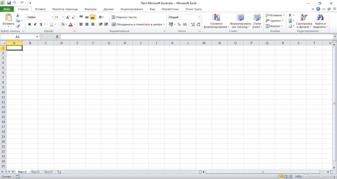
По умолчанию в каждой книге присутствует один лист (в ранних версиях — три листа). Количество листов, которые можно создавать в одной книге, ограничено только возможностями оперативной памяти компьютера. Поле Excel представляет собой таблицу из ячеек. Каждая ячейка имеет свой уникальный адрес, образованный пересечением строк и столбцов. Всего в Excel 1 048 576 строк и 16 384 столбца, что дает 2 147 483 648 ячеек. Над полем с ячейками находится строка функций, в которой отображаются данные, внесенные в ячейки или формулы. Также в программе есть несколько вкладок, которые мы разберем подробнее.
«Файл». С помощью этой вкладки можно отправить документы на печать, установить параметры работы в программе и сделать другие базовые настройки.
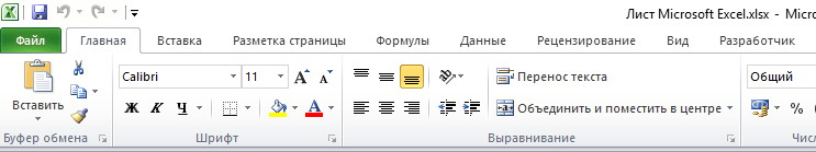
«Главная». Здесь располагается основной набор функций: возможность смены параметров шрифта, сортировка данных, простейшие формулы и правила условного форматирования.
«Вставка». Вкладка предназначена для добавления графических элементов на лист. Пользователь может как добавить обычные рисунки и фотографии, так и создать 2D- и 3D-объекты через конструктор. Кроме того, один из самых важных разделов программы — графики и диаграммы — также находится здесь.
«Разметка страницы». Здесь пользователь может менять формат итогового файла, работать с темой и подложкой.
«Формулы». Все формулы и функции, с которыми пользователь может работать в программе, собраны в этой вкладке и рассортированы по соответствующим разделам.
«Данные». Вкладка помогает с фильтрацией текстовых и числовых значений в таблицах, позволяет импортировать данные из других источников.
«Рецензирование». Здесь можно оставлять примечания к ячейкам, а также устанавливать защиту листа и всей книги.
«Вид». На этой вкладке можно добавлять или убирать сетку таблицы, масштабировать значения, закреплять группы данных в таблицах.
«Разработчик». Дополнительная вкладка, которая не включена по умолчанию. Позволяет работать с Visual Basic, создавать новые макросы и запускать уже имеющиеся.
Форматы файлов
Для Excel существует несколько форматов готовых файлов, которые определяют возможности книги:
- .xlsx — стандартная рабочая книга. Пришла на смену бинарному формату .xls с версии 2007 года;
- .xlsm — рабочая книга, позволяющая работать с макросами;
- .xlsb — рабочая книга, использующая бинарный формат, но одновременно и поддерживающая макросы. Обычно используется при работе с большими таблицами;
- .xltm — шаблон-основа для рабочих книг. Имеется поддержка макросов;
- .xlam — надстройка, созданная для добавления дополнительного функционала.
Нужно учитывать, что некоторые формулы и функции из новых версий могут не работать в старых.
Стандартные операции с ячейками
Активной считается ячейка, которая имеет черную рамку выделения с квадратом в правом нижнем углу. Чтобы вносить данные в ячейку, не обязательно делать по ней дополнительные клики мышью. Вносить данные можно как непосредственно в ячейку, так и через строку формул. При перемещении курсора с помощью клавиш-стрелок активной становится соседняя ячейка, текст в предыдущей сохраняется. Чтобы изменить уже имеющийся текст, необходимо дважды кликнуть по ячейке или внести правки через строку формул.
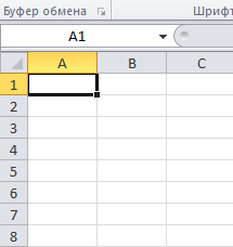
При двойном клике по черному квадрату в правом нижнем углу текстовые данные протянутся до нижнего края созданной таблицы. Если выделить диапазон с последовательными значениями (числа, даты, дни недели), они автоматически пересчитаются в сторону увеличения, заполнив столбец до нижнего края таблицы. Те же операции можно проделать и вручную, протянув за квадрат в нижнем правом углу. В этом случае пользователь самостоятельно определяет границы заполнения.
Чтобы выделить несколько ячеек одновременно, нужно зажать клавишу Ctrl и выбрать нужные ячейки или диапазоны ячеек. Ту же самую операцию можно проделать со строками и столбцами, выделяя необходимое их количество.
Excel автоматически суммирует значения в ячейках, показывая результат в правом нижнем углу листа. Также пользователю предлагаются средние значения данных и общее количество заполненных ячеек.
Ширину столбцов и высоту строк можно менять как вручную, передвигая край столбца/строки, так и нажав правую клавишу мыши и выбрав меню «Ширина столбца (высота строки)». По умолчанию значение ширины указывает на количество символов текущего размера шрифта, которые могут разместиться в ячейке, а значение высоты — на максимально возможный размер шрифта для этой строки.
Ячейки можно объединять с помощью соответствующего меню на вкладке «Главная». Всего существует три варианта объединения:
- объединить и поместить в центре;
- объединить по строкам;
- объединить ячейки.
Следует помнить, что при объединении может нарушаться сортировка данных в таблицах, а также могут некорректно считаться формулы.
Работа с формулами Excel
Главная функция программы — возможность подсчета значений с помощью встроенных формул и функций. Среди них есть простые, позволяющие подсчитать сумму в диапазоне, среднее значение в диапазоне, количество заполненных ячеек и т.д. Есть и более сложные, способные вычислять количество дней между разными датами (в т.ч. рабочих), максимальные и минимальные значения в диапазоне. Работа с функциями и формулами также напрямую зависит от формата ячеек. По умолчанию для всех ячеек установлен общий формат, позволяющий работать как с числовыми, так и с текстовыми данными. Но для более сложной работы он может быть заменен на числовой, процентный, дату, денежный, финансовый, дробный и т.д.
Формула вводится либо через строку функций над таблицей, либо в самой ячейке при двойном клике. В начале функции обязательно должен стоять знак «=». После этого при вводе названия функции появляется помощник, который предлагает выбрать функции из списка. Разберем это на примере формулы средней сложности «СЧЕТЕСЛИ».
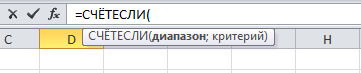
В скобках после функции будут прописаны условия, по которым формула будет проводить вычислениях. Подсказка указывает на то, что потребуется задать диапазон вычислений и критерий, по которому они будут производиться.
Например, нам необходимо подсчитать количество букв «А» в указанном диапазоне:
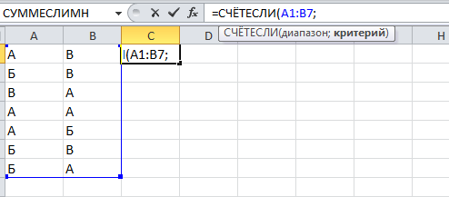
Выделяем диапазон, отмечаем первое условие с помощью знака «;»
Далее выделяем критерий. Его можно прописать вручную, заключив в кавычки; можно выделить ячейку, в которой этот критерий прописан.
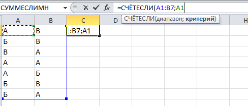
Закрываем скобку, потому что все условия указаны, и нажимаем Enter.
В ячейке C1 получаем ответ: в шести ячейках нашей таблицы написана буква «А».
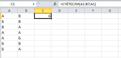
В случае ошибки в формулах в ячейке будет прописано «#ДЕЛ/0!». В этом случае необходимо перепроверить формулу на предмет неточностей и на корректность.
Excel может проводить вычисления не только на активном листе. Для этого при вводе формулы через строку функций нужно перейти на нужный лист и указать ячейку, с которой нужно провести расчет. При протягивании формул автоматически подтянутся и адреса всех ячеек. Чтобы этого не произошло и формулы были подсчитаны корректно, можно закрепить нужную ячейку, выделив ее адрес и нажав клавишу F4. Формат адреса будет выглядеть так: $A$1.
Microsoft Excel know-how is so expected that it hardly warrants a line on a resume anymore. But how well do you really know how to use it?
Marketing is more data-driven than ever before. At any time you could be tracking growth rates, content analysis, or marketing ROI. You may know how to plug in numbers and add up cells in a column in Excel, but that’s not going to get you far when it comes to metrics reporting.
![Download 10 Excel Templates for Marketers [Free Kit]](https://no-cache.hubspot.com/cta/default/53/9ff7a4fe-5293-496c-acca-566bc6e73f42.png)
Do you want to understand what pivot tables are? Are you ready for your first VLOOKUP? Aspiring Excel wizard, read on or jump to the section that interests you most:
What is Microsoft Excel?
Microsoft Excel is a popular spreadsheet software program for business. It’s used for data entry and management, charts and graphs, and project management. You can format, organize, visualize, and calculate data with this tool.
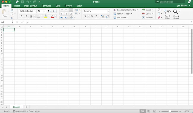
How to Download Microsoft Excel
It’s easy to download Microsoft Excel. First, check to make sure that your PC or Mac meets Microsoft’s system requirements. Next, sign in and install Microsoft 365.
After you sign in, follow the steps for your account and computer system to download and launch the program.
For example, say you’re working on a Mac desktop. You’ll click on Launchpad or look in your applications folder. Then, click on the Excel icon to open the application.
Microsoft Excel Spreadsheet Basics
Sometimes, Excel seems too good to be true. Need to combine data in multiple cells? Excel can do it. Need to copy formatting across an array of cells? Excel can do that, too.
Let’s start this Excel guide with the basics. Once you have these functions down, you’ll be ready to tackle more pro Excel tips and advanced lessons.
Inserting Rows or Columns
As you work with data, you might find yourself needing to add more rows and columns. Doing this one at a time would be super tedious. Luckily, there’s an easier way.
To add multiple rows or columns in a spreadsheet, highlight the number of pre-existing rows or columns that you want to add. Then, right-click and select «Insert.»
In this example, I add three rows to the top of my spreadsheet.
Autofill
Autofill lets you quickly fill adjacent cells with several types of data, including values, series, and formulas.
There are many ways to deploy this feature, but the fill handle is among the easiest.
First, choose the cells you want to be the source. Next, find the fill handle in the lower-right corner of the cell. Then either drag the fill handle to cover the cells you want to fill or just double-click.
Filters
When you’re looking at large data sets, you usually don’t need to look at every row at the same time. Sometimes, you only want to look at data that fit into certain criteria. That’s where filters come in.
Filters allow you to pare down data to only see certain rows at one time. In Excel, you can add a filter to each column in your data. From there, you can choose which cells you want to view.
To add a filter, click the Data tab and select «Filter.» Next, click the arrow next to the column headers. This lets you choose whether you want to organize your data in ascending or descending order, as well as which rows you want to show.
Let’s take a look at the Harry Potter example below. Say you only want to see the students in Gryffindor. By selecting the Gryffindor filter, the other rows disappear.
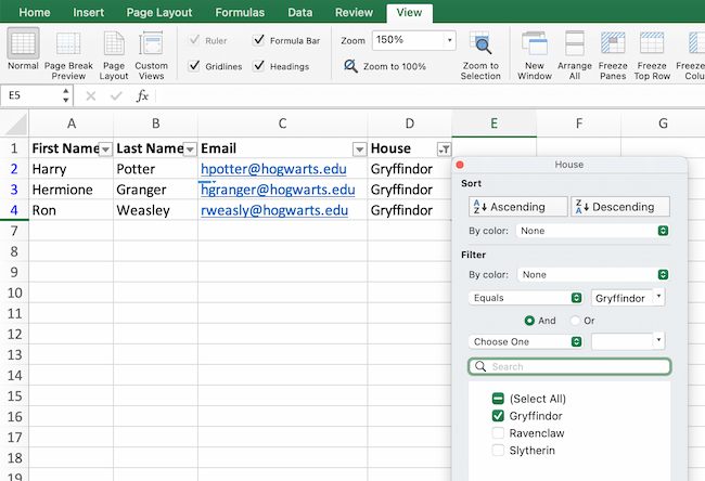
Pro tip: Start with a filtered view in your original spreadsheet. Then, copy and paste the values to another spreadsheet before you start analyzing.
Sort
Sometimes you’ll have a disorganized list of data. This is typical when you’re exporting lists, like marketing contacts or blog posts. Excel’s sort feature can help you alphabetize any list.
Click on the data in the column you want to sort. Then click on the «Data» tab in your toolbar and look for the «Sort» option on the left.
- If the «A» is on top of the «Z,» you can just click on that button once. Choosing A-Z means the list will sort in alphabetical order.
- If the «Z» is on top of the «A,» click the button twice. Z-A selection means the list will sort in reverse alphabetical order.
Remove Duplicates
Large datasets tend to have duplicate content. For example, you may have a list of different company contacts, but you only want to see the number of companies you have. In situations like this, removing duplicates comes in handy.
To remove duplicates, highlight the row or column where you noticed duplicate data. Then, go to the Data tab, and select «Remove Duplicates» (under Tools). A pop-up will appear so that you can confirm which data you want to keep. Select «Remove Duplicates,» and you’re good to go.
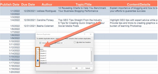
If you want to see an example, this post offers step-by-step instructions for removing duplicates.
You can also use this feature to remove an entire row based on a duplicate column value. So, say you have three rows of information and you only need to see one, you can select the whole dataset and then remove duplicates. The resulting list will have only unique data without any duplicates.
Paste Special
It’s often helpful to change the items in a row of data into a column (or vice versa). It would take a lot of time to copy and paste each individual header.
Not to mention, you may easily fall into one of the biggest, most unfortunate Excel traps — human error. Read here to check out some of the most common Microsoft Excel errors.
Instead of making one of these errors, let Excel do the work for you. Take a look at this example:
To use this function, highlight the column or row you want to transpose. Then, right-click and select «Copy.»
Next, select the cells where you want the first row or column to begin. Right-click on the cell, and then select «Paste Special.»
When the module appears, choose the option to transpose.
Paste Special is a super useful function. In the module, you can also choose between copying formulas, values, formats, or even column widths. This is especially helpful when it comes to copying the results of your pivot table into a chart.
Text to Columns
What if you want to split out information that’s in one cell into two different cells? For example, maybe you want to pull out someone’s company name through their email address. Or you want to separate someone’s full name into a first and last name for your email marketing templates.
Thanks to Microsoft Excel, both are possible. First, highlight the column where you want to split up. Next, go to the Data tab and select «Text to Columns.» A module will appear with more information. First, you need to select either «Delimited» or «Fixed Width.»
- Delimited means you want to break up the column based on characters such as commas, spaces, or tabs.
- Fixed Width means you want to select the exact location in all the columns where you want the split to occur.
Select «Delimited» to separate the full name into first name and last name.
Then, it’s time to choose the delimiters. This could be a tab, semicolon, comma, space, or something else. (For example, «something else» could be the «@» sign used in an email address.) Let’s choose the space for this example. Excel will then show you a preview of what your new columns will look like.
When you’re happy with the preview, press «Next.» This page will allow you to select Advanced Formats if you choose to. When you’re done, click «Finish.»
Format Painter
Excel has a lot of features to make crunching numbers and analyzing your data quick and easy. But if you ever spent some time formatting a spreadsheet, you know it can get a bit tedious.
Don’t waste time repeating the same formatting commands over and over again. Use the format painter to copy formatting from one area of the worksheet to another.
To do this, choose the cell you’d like to replicate. Then, select the format painter option (paintbrush icon) from the top toolbar. When you release the mouse, your cell should show the new format.
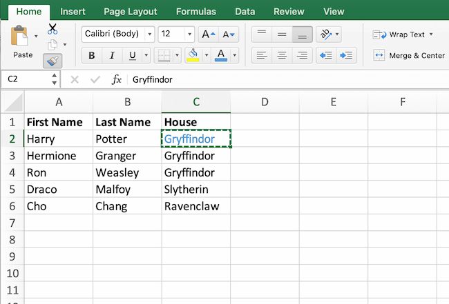
Keyboard Shortcuts
Creating reports in Excel is time-consuming enough. How can we spend less time navigating, formatting, and selecting items in our spreadsheet? Glad you asked. There are a ton of Excel shortcuts out there, including some of our favorites listed below.
Create a New Workbook
PC: Ctrl-N | Mac: Command-N
Select Entire Row
PC: Shift-Space | Mac: Shift-Space
Select Entire Column
PC: Ctrl-Space | Mac: Control-Space
Select Rest of Column
PC: Ctrl-Shift-Down/Up | Mac: Command-Shift-Down/Up
Select Rest of Row
PC: Ctrl-Shift-Right/Left | Mac: Command-Shift-Right/Left
Add Hyperlink
PC: Ctrl-K | Mac: Command-K
Open Format Cells Window
PC: Ctrl-1 | Mac: Command-1
Autosum Selected Cells
PC: Alt-= | Mac: Command-Shift-T
Excel Formulas
At this point, you’re getting used to Excel’s interface and flying through quick commands on your spreadsheets.
Now, let’s dig into the core use case for the software: Excel formulas. Excel can help you do simple arithmetic like adding, subtracting, multiplying, or dividing any data.
- To add, use the + sign.
- To subtract, use the — sign.
- To multiply, use the * sign.
- To divide, use the / sign.
- To use exponents, use the ^ sign.
Remember, all formulas in Excel must begin with an equal sign (=). Use parentheses to make sure certain calculations happen first. For example, consider how =10+10*10 is different from =(10+10)*10.
Besides manually typing in simple calculations, you can also refer to Excel’s built-in formulas. Some of the most common include:
- Average: =AVERAGE(cell range)
- Sum: =SUM(cell range)
- Count: =COUNT(cell range)
Also note that series’ of specific cells are separated by a comma (,), while cell ranges are notated with a colon (:). For example, you could use any of these formulas:
- =SUM(4,4)
- =SUM(A4,B4)
- =SUM(A4:B4)
Conditional Formatting
Conditional formatting lets you change a cell’s color based on the information within the cell. For example, say you want to flag a category in your spreadsheet.
To get started, highlight the group of cells you want to use conditional formatting on. Then, choose «Conditional Formatting» from the Home menu. Next, select a logic option from the dropdown. A window will pop up that prompts you to provide more information about your formatting rule. Select «OK» when you’re done, and you should see your results automatically appear.
Note: You can also create your own logic if you want something beyond the dropdown choices.
Dollar Signs
Have you ever seen a dollar sign in an Excel formula? When this symbol is in a formula, it isn’t representing an American dollar. Instead, it makes sure that the exact column and row stay the same even if you copy the same formula in adjacent rows.
You see, a cell reference — when you refer to cell A5 from cell C5, for example — is relative by default.
This means you’re actually referring to a cell that’s five columns to the left (C minus A) and in the same row (5). This is called a relative formula.
When you copy a relative formula from one cell to another, it’ll adjust the values in the formula based on where it’s moved. But sometimes, you want those values to stay the same no matter whether they’re moved around or not. You can do that by making the formula in the cell into what’s called an absolute formula.
To change the relative formula (=A5+C5) into an absolute formula, precede the row and column values with dollar signs, like this: (=$A$5+$C$5).
Combine Cells Using «&»
Databases tend to split out data to make it as exact as possible. For example, instead of having data that shows a person’s full name, a database might have the data as a first name and then a last name in separate columns.
In Excel, you can combine cells with different data into one cell by using the «&» sign in your function. The example below uses this formula: =A2&» «&B2.
Let’s go through the formula together using an example. So, let’s combine first names and last names into full names in a single column.
To do this, put your cursor in the blank cell where you want the full name to appear. Next, highlight one cell that contains a first name, type in an «&» sign, and then highlight a cell with the corresponding last name.
But you’re not finished. If all you type in is =A2&B2, then there will not be a space between the person’s first name and last name. To add that necessary space, use the function =A2&» «&B2. The quotation marks around the space tell Excel to put a space between the first and last name.
To make this true for multiple rows, drag the corner of that first cell downward as shown in the example.
Pivot Tables
Pivot tables reorganize data in a spreadsheet. A pivot table won’t change the data that you have, but it can sum up values and compare information in a way that’s easy to understand.
For example, let’s look at how many people are in each house at Hogwarts.
To create the Pivot Table, go to Insert > Pivot Table. Excel will automatically populate your pivot table, but you can always change the order of the data. Then, you have four options to choose from.
Report Filter
This allows you to only look at certain rows in your dataset.
For example, to create a filter by house, choose only students in Gryffindor.
Column and Row Labels
These could be any headers or rows in the dataset.
Note: Both Row and Column labels can contain data from your columns. For example, you can drag First Name to either the Row or Column label depending on how you want to see the data.
Value
This section allows you to convert data into a number. Instead of just pulling in any numeric value, you can sum, count, average, max, min, count numbers, or do a few other manipulations with your data. By default, when you drag a field to Value, it always does a count.
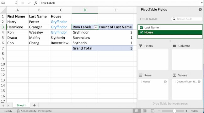
The example above counts the number of students in each house. To recreate this pivot table, go to the pivot table and drag the House column to both the row Labels and the values. This will sum up the number of students associated with each house.
IF Functions
At its most basic level, Excel’s IF function lets you see if a condition you set is true or false for a given value.
If the condition is true, you get one result. If the condition is false, you get another result.
This popular tool is useful for comparisons and finding errors. But if you’re new to Excel you may need a little more information to get the most out of this feature.
Let’s take a look at this function’s syntax:
- =IF(logical_test, value_if_true, [value_if_false])
- With values, this could be: =IF(A2>B2, «Over Budget», «OK»)
In this example, you want to find where you’re overspending. With this IF function, if your spending (what’s in A2) is greater than your budget (what’s in B2), that overspending will be easy to see. Then you can then filter the data so that you see only the line items where you’re going over budget.
The real power of the IF function comes when you string or «nest» multiple IF statements together. This allows you to set multiple conditions, get more specific results, and organize your data into more manageable chunks.
For example, ranges are one way to segment your data for better analysis. For example, you can categorize data into values that are less than 10, 11 to 50, or 51 to 100.
- =IF(B3<11,»10 or less»,IF(B3<51,»11 to 50″,IF(B3<100,»51 to 100″)))
Let’s talk about a few more IF functions.
COUNTIF Function
The power of IF functions goes beyond simple true and false statements. With the COUNTIF function, Excel can count the number of times a word or number appears in any range of cells.
For example, let’s say you want to count the number of times the word «Gryffindor» appears in this data set.
Take a look at the syntax.
- The formula: =COUNTIF(range, criteria)
- The formula with variables from the example below: =COUNTIF(D:D,»Gryffindor»)
In this formula, there are several variables:
Range
The range that you want the formula to cover.
In this one-column example, «D:D» shows that the first and last columns are both D. If you want to look at columns C and D, use «C:D.»
Criteria
Whatever number or piece of text you want Excel to count.
Only use quotation marks if you want the result to be text instead of a number. In this example, «Gryffindor» is the only criteria.
To use this function, type the COUNTIF formula in any cell and press «Enter.» Using the example above, this action will show how many times the word «Gryffindor» appears in the dataset.
SUMIF Function
Ready to make the IF function a bit more complex? Let’s say you want to analyze the number of leads your blog has generated from one author, not the entire team.
With the SUMIFS function, you can add up cells that meet certain criteria. You can add as many different criteria to the formula as you like.
Here’s your formula:
- =SUMIFS(sum_range, criteria_range1, criteria1, [criteria_range2, criteria 2],etc.)
That’s a lot of criteria. Let’s take a look at each part:
Sum_range
The range of cells you’re going to add up.
Criteria_range1
The range that is being searched for your first value.
Criteria1
This is the specific value that determines which cells in Criteria_range1 to add together.
Note: Remember to use quotation marks if you’re searching for text.
In the example below, the SUMIF formula counts the total number of house points from Gryffindor.

If AND/OR
The OR and AND functions round out your IF function choices. These functions check multiple arguments. It returns either TRUE or FALSE depending on if at least one of the arguments is true (this is the OR function), or if all of them are true (this is the AND function).
Lost in a sea of «and’s» and «or’s»? Don’t check out yet. In practice, OR and AND functions will never be used on their own. They need to be nested inside of another IF function. Recall the syntax of a basic IF function:
- =IF(logical_test, value_if_true, [value_if_false])
- Now, let’s fit an OR function inside of the logical_test: =IF(OR(logical1, logical2), value_if_true, [value_if_false])
To put it plainly, this combined formula allows you to return a value if both conditions are true, as opposed to just one. With AND/OR functions, your formulas can be as simple or complex as you want them to be, as long as you understand the basics of the IF function.
VLOOKUP
Have you ever had two sets of data on two different spreadsheets that you want to combine into a single spreadsheet?
For example, say you have a list of names and email addresses in one spreadsheet and a list of email addresses and company names in a different spreadsheet. But you want the names, email addresses, and company names of those people to appear in one spreadsheet.
VLOOKUP is a great go-to formula for this.
Before you use the formula, be sure that you have at least one column that appears identically in both places.
Note: Scour your data sets to make sure the column of data you’re using to combine spreadsheets is exactly the same. This includes removing any extra spaces.
In the example below, Sheet One and Sheet Two are both lists with different information about the same people. The common thread between the two is their email addresses. Let’s combine both datasets so that all the house information from Sheet Two translates over to Sheet One.
Type in the formula: =VLOOKUP(C2,Sheet2!A:B,2,FALSE). This will bring all the house data into Sheet One.
Now that you’ve seen how VLOOKUP works, let’s review the formula.
- The formula: =VLOOKUP(lookup value, table array, column number, [range lookup])
- The formula with variables from the example: =VLOOKUP(C2,Sheet2!A:B,2,FALSE)
In this formula, there are several variables.
Lookup Value
A value that LOOKUP searches for in an array. So, your lookup value is the identical value you have in both spreadsheets.
In the example, the lookup value is the first email address on the list, or cell 2 (C2).
Table Array
Table arrays hold column-oriented or tabular data, like the columns on Sheet Two you’re going to pull your data from.
This table array includes the column of data identical to your lookup value in Sheet One and the column of data you’re trying to copy to Sheet Two.
In the example, «A» means Column A in Sheet Two. The «B» means Column B.
So, the table array is «Sheet2!A:B.»
Column Number
Excel refers to columns as letters and rows as numbers. So, the column number is the selected column for the new data you want to copy.
In the example, this would be the «House» column. «House» is column 2 in the table array.
Note: Your range can be more than two columns. For example, if there are three columns on Sheet Two — Email, Age, and House — and you also want to bring House onto Sheet One, you can still use a VLOOKUP. You just need to change the «2» to a «3» so it pulls back the value in the third column. The formula for this would be: =VLOOKUP(C2:Sheet2!A:C,3,false).]
Range Lookup
This term means that you’re looking for a value within a range of values. You can also use the term «FALSE» to pull only exact value matches.
Note: VLOOKUP will only pull back values to the right of the column containing your identical data on the second sheet. This is why some people prefer to use the INDEX and MATCH functions instead.
INDEX MATCH
Like VLOOKUP, the INDEX and MATCH functions pull data from another dataset into one central location. Here are the main differences:
VLOOKUP is a much simpler formula.
If you’re working with large datasets that need thousands of lookups, the INDEX MATCH function will decrease load time in Excel.
INDEX MATCH formulas work right-to-left.
VLOOKUP formulas only work as a left-to-right lookup. So, if you need to do a lookup that has a column to the right of the results column, you’d have to rearrange those columns to do a VLOOKUP. This can be tedious with large datasets and lead to errors.
Let’s look at an example. Let’s say Sheet One contains a list of names and their Hogwarts email addresses. Sheet Two contains a list of email addresses and each student’s Patronus.
The information that lives in both sheets is the email addresses column. But, the column numbers for email addresses are different on the two sheets. So, you’d use the INDEX MATCH formula instead of VLOOKUP to avoid column-switching errors.
The INDEX MATCH formula is the MATCH formula nested inside the INDEX formula.
- The formula: =INDEX(table array, MATCH formula)
- This becomes: =INDEX(table array, MATCH (lookup_value, lookup_array))
- The formula with variables from the example: =INDEX(Sheet2!A:A,(MATCH(Sheet1!C:C,Sheet2!C:C,0)))
Here are the variables:
Table Array
The range of columns on Sheet Two that contain the new data you want to bring over to Sheet One.
In the example, «A» means Column A, and has the «Patronus» information for each person.
Lookup Value
This Sheet One column has identical values in both spreadsheets.
In the example, this is the «email» column on Sheet One, which is Column C. So, Sheet1!C:C.
Lookup Array
Again, an array is a group of values in rows and columns that you want to search.
In this example, the lookup array is the column in Sheet Two that contains identical values in both spreadsheets. So, the «email» column on Sheet Two, Sheet2!C:C.
Once you have your variables set, type in the INDEX MATCH formula. Add it where you want the combined information to populate.
Data Visualization
Now that you’ve learned formulas and functions, let’s make your analysis visual. With a beautiful graph, your audience will be able to process and remember your data more easily.
Create a Basic Graph
First, decide what type of graph to use. Bar charts and pie charts help you compare categories. Pie charts compare part of a whole and are often best when one of the categories is way larger than the others. Bar charts highlight incremental differences between categories. Finally, line charts can help display trends over time.
This post can help you find the best chart or graph for your presentation.
Next, highlight the data you want to turn into a chart. Then choose «Charts» in the top navigation. You can also use Insert > Chart if you have an older version of Excel. Then you can adjust and resize your chart until it makes the statement you’re hoping for.
Microsoft Excel Can Help Your Business Grow
Excel is a useful tool for any small business. Whether you’re focused on marketing, HR, sales, or service, these Microsoft Excel tips can boost your performance.
Whether you want to improve efficiency or productivity, Excel can help. You can find new trends and organize your data into usable insights. It can make your data analysis easier to understand and your daily tasks easier.
All it takes is a little know-how and some time with the software. So start learning, and get ready to grow.
Editor’s note: This post was originally published in April 2018 and has been updated for comprehensiveness.

Powerful and complex, Microsoft Excel comes packed with so many tools that it’s often hard to know which tool can solve a particular problem. Ever feel like it’s easier to just keep doing things the slow way simply because it works? But you deserve better than that, so we’ve gathered five essential Excel tools that save you time and effort. If you’re not currently using them, it’s time to up your game.
Jump to:
- Five Excel tools you should use
- Flash fill
- Filter and calculate with tables
- Dropdown lists
- Isolate variable data in a data area
- Exception reporting with conditional formatting
Five Excel tools you should use
1. Flash fill
Excel’s Flash Fill feature makes it easy to fill data in an Excel worksheet based on adjacent data patterns. Flash Fill looks at the surrounding data, and then it fills a range based on what it finds. You might, for example, use Flash Fill to separate names (or to join them together) when you have a column or columns of name data in the wrong format.
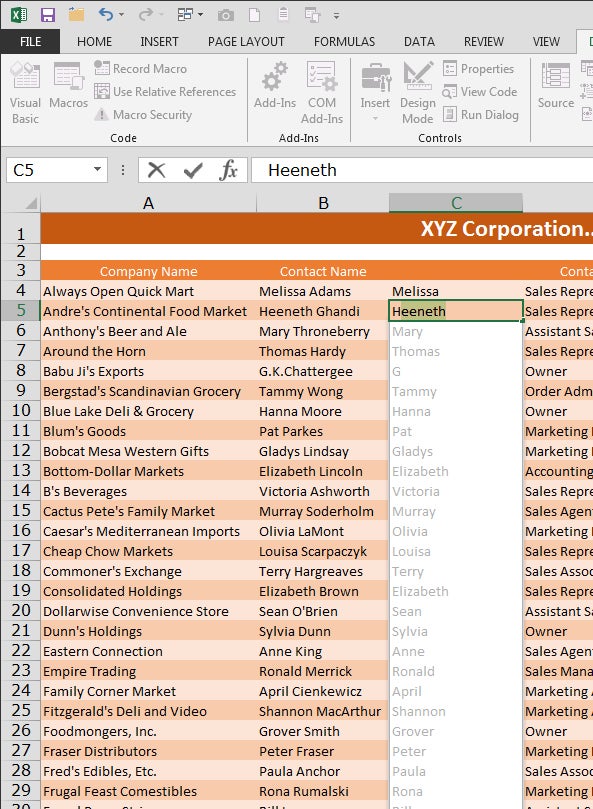
When you need to arrange existing data differently, Flash Fill can do in seconds what might otherwise take hours of manual work.
How to use Flash Fill: Create one or more empty columns alongside the existing data. Start typing the data that you want to see in the column. As you proceed, Excel looks for a pattern and, when it sees it, it enters the remaining data automatically for you. If Excel gets it right, all is good.
If it doesn’t, then continue; edit the entries it didn’t get right, and Excel will adjust the filled data according to the new pattern. You can also access Flash Fill from the Data tab on the Ribbon. Flash Fill can save you hours of manual work and avoid the need to write custom macro solutions.
2. Filter and calculate with tables
When you’re working with lists of data in Excel, the Format-as-Table option (in the Styles area of the Home tab) does a lot more than simply format your data. When you click in a list of data and apply a table format to the data using this tool, Excel also adds a filter to each column.
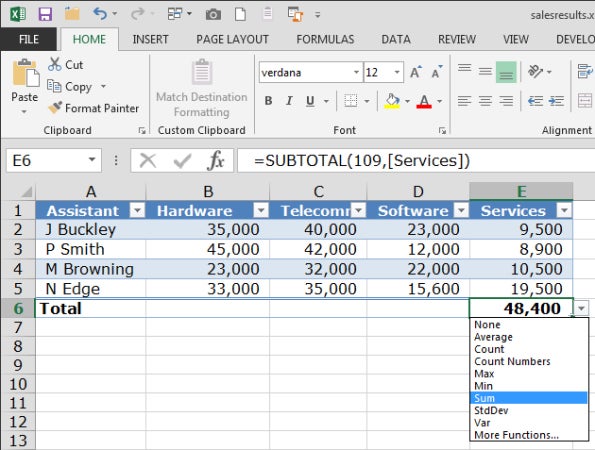
The Format-as-Table option does much more than apply simple formatting to list data.
You can use this to sort and filter the data. From the Table Tools > Design Tab you can set special formatting for columns and rows within the table, and then click Total Row to add a total row. When you then click in a cell in the total row, a dropdown list appears from which you can select a function to apply to that column of data, such as sum, average, count and so on.
Excel creates these calculations using a subtotal function, which means they show results for visible data only. And when you create a chart based on the table data, that chart is dynamic and will expand to include any data that you add to the table in future.
3. Dropdown lists
When you’re typing data into a list—and if one or more cells above contain that same data—you can enter it using a dropdown list. Simply click in the cell and press Alt + Down Arrow and a list of contents from the cells above the current cell will appear. Click the entry you want to use and press Enter. This speeds up the data-entering process, but it also ensures data entry consistency.
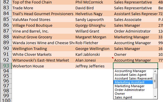
You can use existing data to speed up data entry or to create custom dropdown lists.
You can also create a custom list by entering the list on a second worksheet. Select the range and name it using the Name box at the left of the formula bar. Now select the column to which you want the list added, choose Data > Data Validation, set it to List, and select the named range as the Source. In the future all the selected cells will contain a dropdown list from which you can select the desired cell entry.
4. Isolate variable data in a data area
When your worksheet uses data—such as tax rates—that may or may not change over time, it’s best to place it in a separate area on the worksheet. You can then refer to those cells in your formulas.
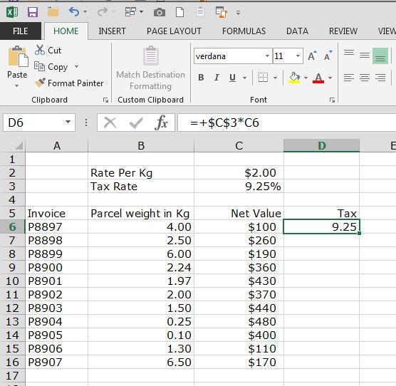
Contain variable data—such as tax rates—in a separate area so that you can easily verify and update values should they change.
For example: place the state tax rate in a cell above your worksheet data and label it clearly. Then refer to that cell in your calculations instead of placing the value inside the calculation. Using a data area ensures that anyone can determine the tax rate by referring to the labeled cell. If tax rates change, you then need only change one cell and not all the calculations in the worksheet. People will understand your worksheets more easily, and that they can be quickly audited for accuracy.
5. Exception reporting with conditional formatting
Most managers who review data in worksheets look for limited amounts of data that does not conform to expectations. When reviewing a debtor list, for example, you’ll be more interested in seeing out-of-the ordinary and excessively high results than values that fall within normal ranges.
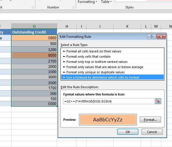
Conditional formatting is a handy way to draw attention to exceptional values that require further attention.
You can draw attention to this type of data using conditional formatting. First determine what exceptions you want to highlight, and then write a rule or rules to isolate this data in your workbook. Conditional formatting is dynamic; if the data changes, the formatting will update automatically. In the example above, we created a conditional format to highlight outstanding amounts that are more than twice the average.
Helen Bradley is a respected international journalist writing regularly for small business and computer publications in the USA, Canada, South Africa, UK and Australia. You can learn more about her at her website, HelenBradley.com
This article was originally published on September 11, 2015. It was updated by Tamara Scott.
Read next: Best Excel Add Ons & Tools You Need in 2021