
IMPORTANT: Ideas in Excel is now Analyze Data
To better represent how Ideas makes data analysis simpler, faster and more intuitive, the feature has been renamed to Analyze Data. The experience and functionality is the same and still aligns to the same privacy and licensing regulations. If you’re on Semi-Annual Enterprise Channel, you may still see «Ideas» until Excel has been updated.

Analyze Data in Excel empowers you to understand your data through natural language queries that allow you to ask questions about your data without having to write complicated formulas. In addition, Analyze Data provides high-level visual summaries, trends, and patterns.
Have a question? We can answer it!
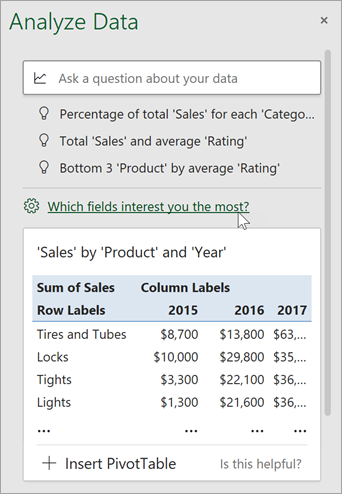
Simply select a cell in a data range > select the Analyze Data button on the Home tab. Analyze Data in Excel will analyze your data, and return interesting visuals about it in a task pane.
If you’re interested in more specific information, you can enter a question in the query box at the top of the pane, and press Enter. Analyze Data will provide answers with visuals such as tables, charts or PivotTables that can then be inserted into the workbook.
If you are interested in exploring your data, or just want to know what is possible, Analyze Data also provides personalized suggested questions which you can access by selecting on the query box.
Try Suggested Questions
Just ask your question
Select the text box at the top of the Analyze Data pane, and you’ll see a list of suggestions based on your data.

You can also enter a specific question about your data.

Notes:
-
Analyze Data is available to Microsoft 365 subscribers in English, French, Spanish, German, Simplified Chinese, and Japanese. If you are a Microsoft 365 subscriber, make sure you have the latest version of Office. To learn more about the different update channels for Office, see: Overview of update channels for Microsoft 365 apps.
-
The Natural Language Queries functionality in Analyze Data is being made available to customers on a gradual basis. It may not be available in all countries or regions at this time.
Get specific with Analyze Data
If you do not have a question in mind, in addition to Natural Language, Analyze Data analyzes and provides high-level visual summaries, trends, and patterns.
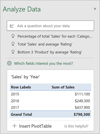
You can save time and get a more focused analysis by selecting only the fields you want to see. When you choose fields and how to summarize them, Analyze Data excludes other available data — speeding up the process and presenting fewer, more targeted suggestions. For example, you might only want to see the sum of sales by year. Or you could ask Analyze Data to display average sales by year.
Select Which fields interest you the most?
Select the fields and how to summarize their data.
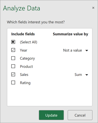
Analyze Data offers fewer, more targeted suggestions.
Note: The Not a value option in the field list refers to fields that are not normally summed or averaged. For example, you wouldn’t sum the years displayed, but you might sum the values of the years displayed. If used with another field that is summed or averaged, Not a value works like a row label, but if used by itself, Not a value counts unique values of the selected field.
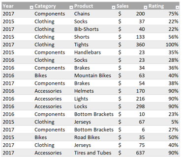
Analyze Data works best with clean, tabular data.
Here are some tips for getting the most out of Analyze Data:
-
Analyze Data works best with data that’s formatted as an Excel table. To create an Excel table, click anywhere in your data and then press Ctrl+T.
-
Make sure you have good headers for the columns. Headers should be a single row of unique, non-blank labels for each column. Avoid double rows of headers, merged cells, etc.
-
If you have complicated, or nested data, you can use Power Query to convert tables with cross-tabs, or multiple rows of headers.
Didn’t get Analyze Data? It’s probably us, not you.
Here are some reasons why Analyze Data may not work on your data:
-
Analyze Data doesn’t currently support analyzing datasets over 1.5 million cells. There is currently no workaround for this. In the meantime, you can filter your data, then copy it to another location to run Analyze Data on it.
-
String dates like «2017-01-01» will be analyzed as if they are text strings. As a workaround, create a new column that uses the DATE or DATEVALUE functions, and format it as a date.
-
Analyze Data won’t work when Excel is in compatibility mode (i.e. when the file is in .xls format). In the meantime, save your file as an .xlsx, .xlsm, or .xlsb file.
-
Merged cells can also be hard to understand. If you’re trying to center data, like a report header, then as a workaround, remove all merged cells, then format the cells using Center Across Selection. Press Ctrl+1, then go to Alignment > Horizontal > Center Across Selection.
Analyze Data works best with clean, tabular data.
Here are some tips for getting the most out of Analyze Data:
-
Analyze Data works best with data that’s formatted as an Excel table. To create an Excel table, click anywhere in your data and then press
 +T.
+T. -
Make sure you have good headers for the columns. Headers should be a single row of unique, non-blank labels for each column. Avoid double rows of headers, merged cells, etc.
 +T.
+T.Didn’t get Analyze Data? It’s probably us, not you.
Here are some reasons why Analyze Data may not work on your data:
-
Analyze Data doesn’t currently support analyzing datasets over 1.5 million cells. There is currently no workaround for this. In the meantime, you can filter your data, then copy it to another location to run Analyze Data on it.
-
String dates like «2017-01-01» will be analyzed as if they are text strings. As a workaround, create a new column that uses the DATE or DATEVALUE functions, and format it as a date.
-
Analyze Data can’t analyze data when Excel is in compatibility mode (i.e. when the file is in .xls format). In the meantime, save your file as an .xlsx, .xlsm, or xslb file.
-
Merged cells can also be hard to understand. If you’re trying to center data, like a report header, then as a workaround, remove all merged cells, then format the cells using Center Across Selection. Press Ctrl+1, then go to Alignment > Horizontal > Center Across Selection.
Analyze Data works best with clean, tabular data.
Here are some tips for getting the most out of Analyze Data:
-
Analyze Data works best with data that’s formatted as an Excel table. To create an Excel table, click anywhere in your data and then click Home > Tables > Format as Table.
-
Make sure you have good headers for the columns. Headers should be a single row of unique, non-blank labels for each column. Avoid double rows of headers, merged cells, etc.
Didn’t get Analyze Data? It’s probably us, not you.
Here are some reasons why Analyze Data may not work on your data:
-
Analyze Data doesn’t currently support analyzing datasets over 1.5 million cells. There is currently no workaround for this. In the meantime, you can filter your data, then copy it to another location to run Analyze Data on it.
-
String dates like «2017-01-01» will be analyzed as if they are text strings. As a workaround, create a new column that uses the DATE or DATEVALUE functions, and format it as a date.
We’re always improving Analyze Data
Even if you don’t have any of the above conditions, we may not find a recommendation. That’s because we are looking for a specific set of insight classes, and the service doesn’t always find something. We are continually working to expand the analysis types that the service supports.
Here is the current list that is available:
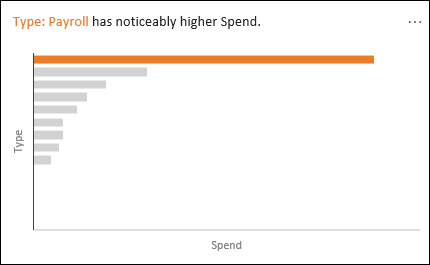
-
Rank: Ranks and highlights the item that is significantly larger than the rest of the items.
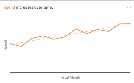
-
Trend: Highlights when there is a steady trend pattern over a time series of data.
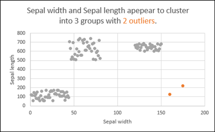
-
Outlier: Highlights outliers in time series.
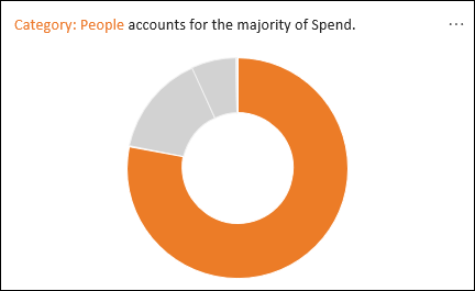
-
Majority: Finds cases where a majority of a total value can be attributed to a single factor.
If you don’t get any results, please send us feedback by going to File > Feedback.
Because Analyze Data analyzes your data with artificial intelligence services, you might be concerned about your data security. You can read the Microsoft privacy statement for more details.
Need more help?
You can always ask an expert in the Excel Tech Community or get support in the Answers community.
Содержание
- Включение блока инструментов
- Активация
- Запуск функций группы «Анализ данных»
- Вопросы и ответы

Программа Excel – это не просто табличный редактор, но ещё и мощный инструмент для различных математических и статистических вычислений. В приложении имеется огромное число функций, предназначенных для этих задач. Правда, не все эти возможности по умолчанию активированы. Именно к таким скрытым функциям относится набор инструментов «Анализ данных». Давайте выясним, как его можно включить.
Включение блока инструментов
Чтобы воспользоваться возможностями, которые предоставляет функция «Анализ данных», нужно активировать группу инструментов «Пакет анализа», выполнив определенные действия в настройках Microsoft Excel. Алгоритм этих действий практически одинаков для версий программы 2010, 2013 и 2016 года, и имеет лишь незначительные отличия у версии 2007 года.
Активация
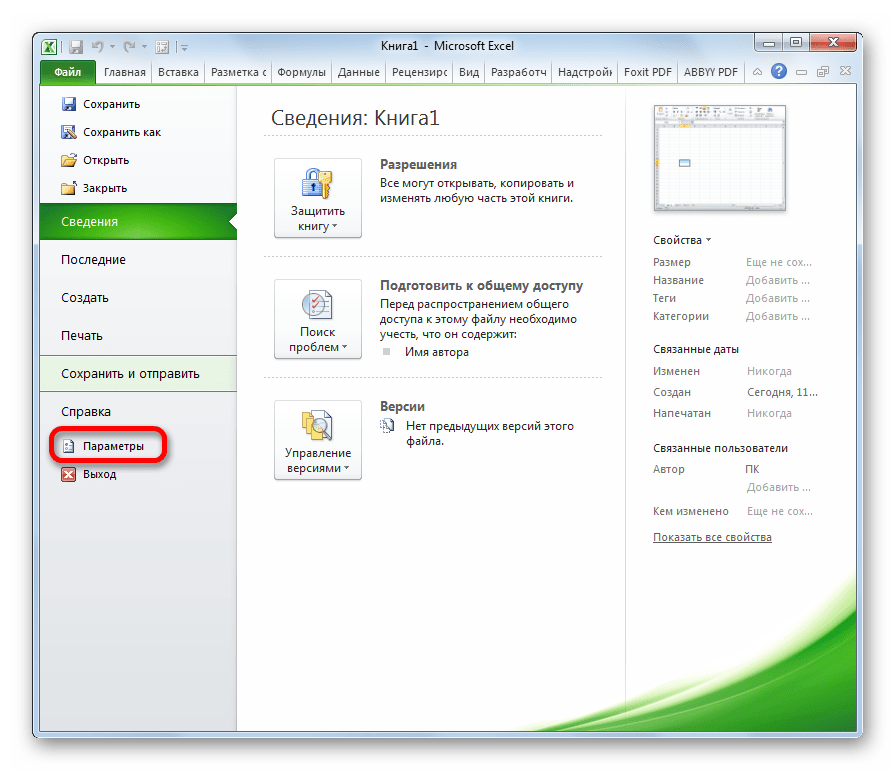
- Перейдите во вкладку «Файл». Если вы используете версию Microsoft Excel 2007, то вместо кнопки «Файл» нажмите значок Microsoft Office в верхнем левом углу окна.
- Кликаем по одному из пунктов, представленных в левой части открывшегося окна – «Параметры».
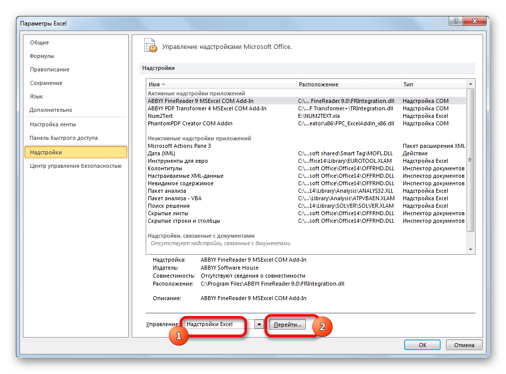
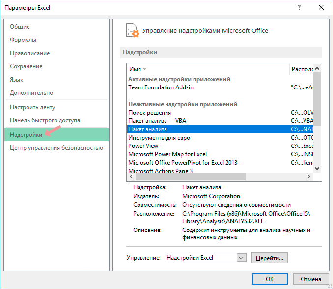
- В открывшемся окне параметров Эксель переходим в подраздел «Надстройки» (предпоследний в списке в левой части экрана).
- В этом подразделе нас будет интересовать нижняя часть окна. Там представлен параметр «Управление». Если в выпадающей форме, относящейся к нему, стоит значение отличное от «Надстройки Excel», то нужно изменить его на указанное. Если же установлен именно этот пункт, то просто кликаем на кнопку «Перейти…» справа от него.
- Открывается небольшое окно доступных надстроек. Среди них нужно выбрать пункт «Пакет анализа» и поставить около него галочку. После этого, нажать на кнопку «OK», расположенную в самом верху правой части окошка.


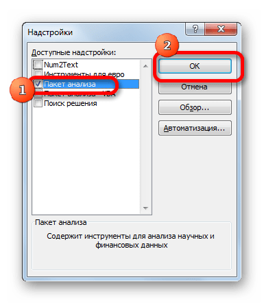
После выполнения этих действий указанная функция будет активирована, а её инструментарий доступен на ленте Excel.
Запуск функций группы «Анализ данных»
Теперь мы можем запустить любой из инструментов группы «Анализ данных».
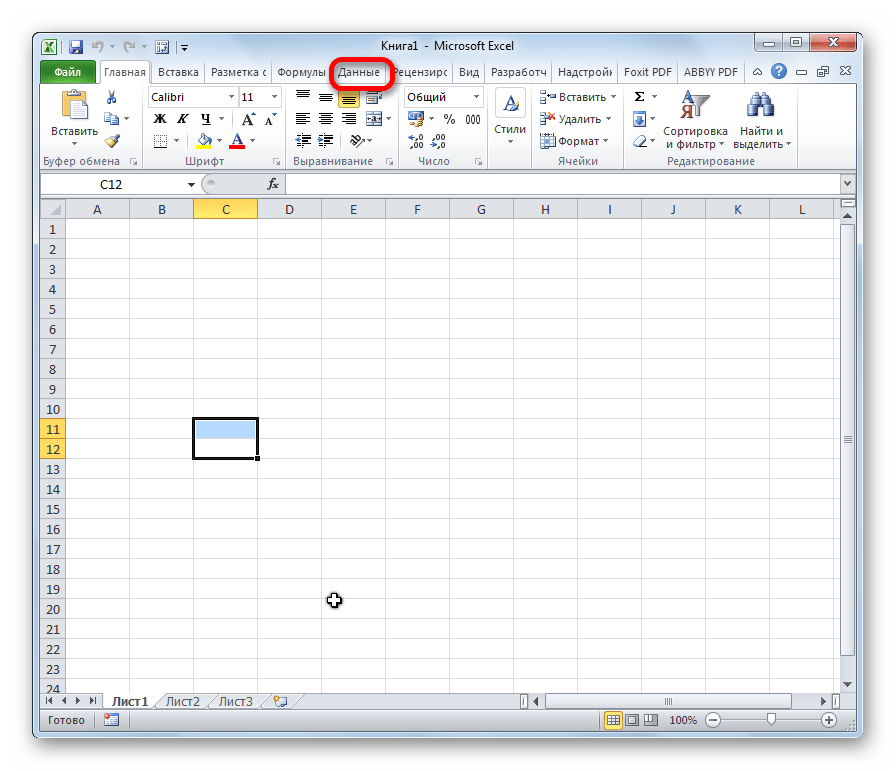
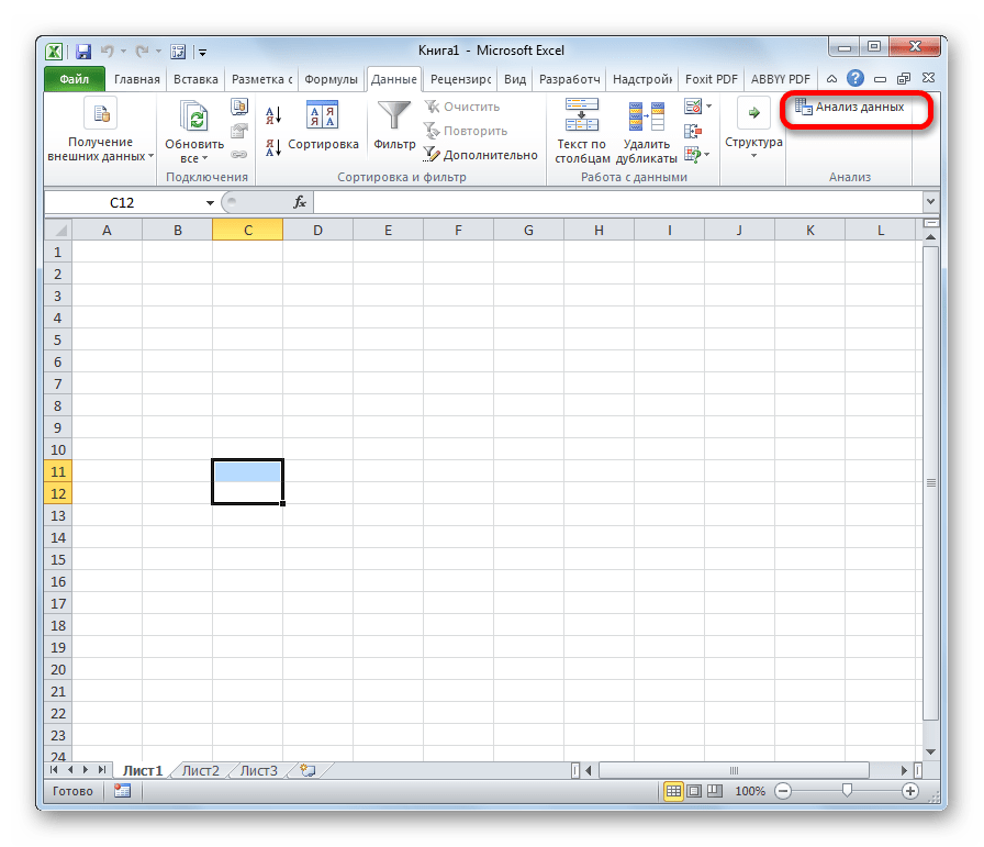
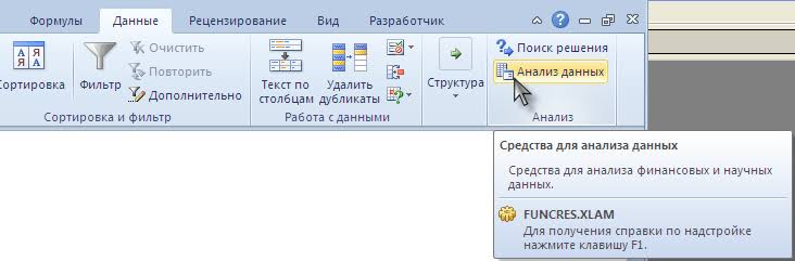
- Переходим во вкладку «Данные».
- В открывшейся вкладке на самом правом краю ленты располагается блок инструментов «Анализ». Кликаем по кнопке «Анализ данных», которая размещена в нём.
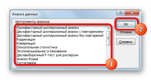
- После этого запускается окошко с большим перечнем различных инструментов, которые предлагает функция «Анализ данных». Среди них можно выделить следующие возможности:
- Корреляция;
- Гистограмма;
- Регрессия;
- Выборка;
- Экспоненциальное сглаживание;
- Генератор случайных чисел;
- Описательная статистика;
- Анализ Фурье;
- Различные виды дисперсионного анализа и др.
Выбираем ту функцию, которой хотим воспользоваться и жмем на кнопку «OK».
Работа в каждой функции имеет свой собственный алгоритм действий. Использование некоторых инструментов группы «Анализ данных» описаны в отдельных уроках.
Урок: Корреляционный анализ в Excel

Урок: Регрессионный анализ в Excel
Урок: Как сделать гистограмму в Excel
Как видим, хотя блок инструментов «Пакет анализа» и не активирован по умолчанию, процесс его включения довольно прост. В то же время, без знания четкого алгоритма действий вряд ли у пользователя получится быстро активировать эту очень полезную статистическую функцию.
Еще статьи по данной теме:
Помогла ли Вам статья?
Questions and answers
- From Excel 2013 or Excel 2016, click the File tab, and then click Options.
- Click Add-Ins and in the Manage box, select Excel Add-ins.
- Click Go…
- In the Add-Ins available: box, select the Analysis ToolPak check box, and then click OK.
Contents
- 1 How do you do data analysis on Excel?
- 2 Where is the quick analysis tool in Excel 2016?
- 3 Can Excel be used for data analysis?
- 4 How do you do a data analysis?
- 5 What is Excel data analysis?
- 6 How do I do a quick analysis in Excel?
- 7 How do you Analyse text in Excel?
- 8 Where can I learn Excel for data analysis?
- 9 What are the 5 steps to the data analysis process?
- 10 What is data analysis example?
- 11 What are the three steps of data analysis?
- 12 Where is data analysis Excel 2019?
- 13 How do you analyze data in words?
- 14 How do you analyze unstructured data in Excel?
- 15 What are the 8 stages of data analysis?
- 16 Which methods are basic data analysis methods?
- 17 What is needed for data analyst?
- 18 What are top 3 skills for data analyst?
- 19 What is the best data analysis method?
- 20 What is data analysis tools?
Click the File tab, click Options, and then click the Add-Ins category. In the Manage box, select Excel Add-ins and then click Go. In the Add-Ins box, check the Analysis ToolPak check box, and then click OK.
Where is the quick analysis tool in Excel 2016?
bottom right corner
If you select your data, the quick analysis button should appear at the bottom right corner of the screen. It can also be accessed by typing Ctrl + Q.
Can Excel be used for data analysis?
Microsoft Excel is one of the top tools for data analysis and the built-in pivot tables are arguably the most popular analytic tool.To complement, pivot charts and slicers can be used together to visualize data and create easy to use dashboards.
How do you do a data analysis?
To improve how you analyze your data, follow these steps in the data analysis process:
- Step 1: Define your goals.
- Step 2: Decide how to measure goals.
- Step 3: Collect your data.
- Step 4: Analyze your data.
- Step 5: Visualize and interpret results.
What is Excel data analysis?
Data Analysis with Excel is a comprehensive tutorial that provides a good insight into the latest and advanced features available in Microsoft Excel. It explains in detail how to perform various data analysis functions using the features available in MS-Excel.
How do I do a quick analysis in Excel?
Choose your chart using Quick Analysis
- Select a range of cells.
- Select the Quick Analysis button that appears at the bottom right corner of the selected data. Or, press Ctrl + Q.
- Select Charts.
- Hover over the chart types to preview a chart, and then select the chart you want.
How do you Analyse text in Excel?
Perform Complex Data Analysis with the Analysis Toolpak
- In Excel, click Options in the File tab.
- Go to Add-ins, then select Analysis ToolPak and click Go.
- In the pop-up window, check the Analysis ToolPak option and click OK.
- Under the Data tab in the toolbar of your Excel sheet, you’ll now see a Data Analysis option.
Where can I learn Excel for data analysis?
Share this:
- Best Excel Data Analysis Courses.
- Coursera.
- DataCamp.
- ed2go.
- Edureka.
- edX.
- Excel Courses.
- Excel Data Analysis Courses.
What are the 5 steps to the data analysis process?
Here, we’ll walk you through the five steps of analyzing data.
- Step One: Ask The Right Questions. So you’re ready to get started.
- Step Two: Data Collection. This brings us to the next step: data collection.
- Step Three: Data Cleaning.
- Step Four: Analyzing The Data.
- Step Five: Interpreting The Results.
What is data analysis example?
A simple example of Data analysis is whenever we take any decision in our day-to-day life is by thinking about what happened last time or what will happen by choosing that particular decision. This is nothing but analyzing our past or future and making decisions based on it.
What are the three steps of data analysis?
These steps and many others fall into three stages of the data analysis process: evaluate, clean, and summarize.
Where is data analysis Excel 2019?
Click the “Data” tab in the main Excel interface, and the “Data Analysis” button can be found in the “Analyze” section of the menu. Clicking the “Data Analysis” button opens a window where all analysis tools are shown.
How do you analyze data in words?
Here’s how to do word counts.
- Step 1 – Find the text you want to analyze.
- Step 2 – Scrub the data.
- Step 3 – Count the words.
- Step 1 – Get the Data into a Spreadsheet.
- Step 2 – Scrub the Responses.
- Step 3 – Assign Descriptors.
- Step 4 – Count the Fragments Assigned to Each Descriptor.
- Step 5 – Repeat Steps 3 and 4.
How do you analyze unstructured data in Excel?
The Keys to parsing in unstructured data:
- To first Assign each row a “Record ID”, that helps with how to treat each row.
- Get rid of the blank rows.
- Use the “Generate Rows” tool to put each Description and Value on a single row, when there are multiple Descriptions and Values on a single row.
What are the 8 stages of data analysis?
data analysis process follows certain phases such as business problem statement, understanding and acquiring the data, extract data from various sources, applying data quality for data cleaning, feature selection by doing exploratory data analysis, outliers identification and removal, transforming the data, creating
Which methods are basic data analysis methods?
Data Analysis Methods
- Qualitative Analysis. This approach mainly answers questions such as ‘why,’ ‘what’ or ‘how.
- Quantitative Analysis. Generally, this analysis is measured in terms of numbers.
- Text analysis.
- Statistical analysis.
- Diagnostic analysis.
- Predictive analysis.
- Prescriptive Analysis.
What is needed for data analyst?
SQL. SQL, or Structured Query Language, is the ubiquitous industry-standard database language and is possibly the most important skill for data analysts to know.Each month, thousands of job postings requiring SQL skills are posted, and the median salary for someone with advanced SQL skills sits well over $75,000.
What are top 3 skills for data analyst?
Below, we’ve listed the top 11 technical and soft skills required to become a data analyst:
- Data Visualization.
- Data Cleaning.
- MATLAB.
- R.
- Python.
- SQL and NoSQL.
- Machine Learning.
- Linear Algebra and Calculus.
What is the best data analysis method?
Two main qualitative data analysis techniques used by data analysts are content analysis and discourse analysis. Another popular method is narrative analysis, which focuses on stories and experiences shared by a study’s participants.
What is data analysis tools?
Data collection and analysis tools are defined as a series of charts, maps, and diagrams designed to collect, interpret, and present data for a wide range of applications and industries.
Надстройка пакета анализа в Excel используется для сложного статистического анализа, например, регрессии, анализа Фурье, дисперсионного анализа, корреляции. По умолчанию пакет анализа в Excel не подключен. Поэтому в этой статье мы рассмотрим, как включить анализ данных в Excel.
- Если вы используете Excel 2010, Excel 2013, Excel 2016, то для того чтобы включить анализ данных, переходим в настройки MS Excel: вкладка «ФАЙЛ» —> пункт «Параметры» —> категория «Надстройки».

Как включить анализ данных в Excel – Включение анализа данных в Excel 2010 — 2016
Если вы пользователь Excel 2007, то щелкните по значку  , и нажмите кнопку «Параметры Excel».

Как включить анализ данных в Excel – Включение анализа данных в Excel 2007
- В открывающемся списке «Управление» выбираем пункт «Надстройки Excel» и нажимаем «Перейти».

Как включить анализ данных в Excel – Управление, Надстройки в Excel
- В открывшемся диалоговом окне выбираем «Пакет анализа» и нажимаем кнопку «ОК».

Как включить анализ данных в Excel – Установка Пакета анализа для генерации случайных чисел
- Теперь анализ данных в Excel доступен и находится во вкладке «ДАННЫЕ», группа «Анализ» —> «Анализ данных».

Как включить анализ данных в Excel – Расположение Анализа данных
В пакет анализа данных включены многие инструменты анализа. Ниже приведен скриншот окна «Анализа данных» со списком некоторых инструментов.

Как включить анализ данных в Excel – Окно Анализа данных
Вот и все. Теперь вы знаете, как включить анализ данных в Excel, и тем самым упростить себе работу в табличном редакторе.
Use the Analysis ToolPak to perform complex data analysis
If you need to develop complex statistical or engineering analyses, you can save steps and time by using the Analysis ToolPak. You provide the data and parameters for each analysis, and the tool uses the appropriate statistical or engineering macro functions to calculate and display the results in an output table. Some tools generate charts in addition to output tables.
The data analysis functions can be used on only one worksheet at a time. When you perform data analysis on grouped worksheets, results will appear on the first worksheet and empty formatted tables will appear on the remaining worksheets. To perform data analysis on the remainder of the worksheets, recalculate the analysis tool for each worksheet.
The Analysis ToolPak includes the tools described in the following sections. To access these tools, click Data Analysis in the Analysis group on the Data tab. If the Data Analysis command is not available, you need to load the Analysis ToolPak add-in program.
Click the File tab, click Options, and then click the Add-Ins category.
In the Manage box, select Excel Add-ins and then click Go.
If you’re using Excel for Mac, in the file menu go to Tools > Excel Add-ins.
In the Add-Ins box, check the Analysis ToolPak check box, and then click OK.
If Analysis ToolPak is not listed in the Add-Ins available box, click Browse to locate it.
If you are prompted that the Analysis ToolPak is not currently installed on your computer, click Yes to install it.
Note: To include Visual Basic for Application (VBA) functions for the Analysis ToolPak, you can load the Analysis ToolPak — VBA Add-in the same way that you load the Analysis ToolPak. In the Add-ins available box, select the Analysis ToolPak — VBA check box.
The Anova analysis tools provide different types of variance analysis. The tool that you should use depends on the number of factors and the number of samples that you have from the populations that you want to test.
Anova: Single Factor
This tool performs a simple analysis of variance on data for two or more samples. The analysis provides a test of the hypothesis that each sample is drawn from the same underlying probability distribution against the alternative hypothesis that underlying probability distributions are not the same for all samples. If there are only two samples, you can use the worksheet function T . TEST. With more than two samples, there is no convenient generalization of T . TEST, and the Single Factor Anova model can be called upon instead.
Anova: Two-Factor with Replication
This analysis tool is useful when data can be classified along two different dimensions. For example, in an experiment to measure the height of plants, the plants may be given different brands of fertilizer (for example, A, B, C) and might also be kept at different temperatures (for example, low, high). For each of the six possible pairs of , we have an equal number of observations of plant height. Using this Anova tool, we can test:
Whether the heights of plants for the different fertilizer brands are drawn from the same underlying population. Temperatures are ignored for this analysis.
Whether the heights of plants for the different temperature levels are drawn from the same underlying population. Fertilizer brands are ignored for this analysis.
Whether having accounted for the effects of differences between fertilizer brands found in the first bulleted point and differences in temperatures found in the second bulleted point, the six samples representing all pairs of values are drawn from the same population. The alternative hypothesis is that there are effects due to specific pairs over and above the differences that are based on fertilizer alone or on temperature alone.
Anova: Two-Factor Without Replication
This analysis tool is useful when data is classified on two different dimensions as in the Two-Factor case With Replication. However, for this tool it is assumed that there is only a single observation for each pair (for example, each pair in the preceding example).
The CORREL and PEARSON worksheet functions both calculate the correlation coefficient between two measurement variables when measurements on each variable are observed for each of N subjects. (Any missing observation for any subject causes that subject to be ignored in the analysis.) The Correlation analysis tool is particularly useful when there are more than two measurement variables for each of N subjects. It provides an output table, a correlation matrix, that shows the value of CORREL (or PEARSON) applied to each possible pair of measurement variables.
The correlation coefficient, like the covariance, is a measure of the extent to which two measurement variables «vary together.» Unlike the covariance, the correlation coefficient is scaled so that its value is independent of the units in which the two measurement variables are expressed. (For example, if the two measurement variables are weight and height, the value of the correlation coefficient is unchanged if weight is converted from pounds to kilograms.) The value of any correlation coefficient must be between -1 and +1 inclusive.
You can use the correlation analysis tool to examine each pair of measurement variables to determine whether the two measurement variables tend to move together — that is, whether large values of one variable tend to be associated with large values of the other (positive correlation), whether small values of one variable tend to be associated with large values of the other (negative correlation), or whether values of both variables tend to be unrelated (correlation near 0 (zero)).
The Correlation and Covariance tools can both be used in the same setting, when you have N different measurement variables observed on a set of individuals. The Correlation and Covariance tools each give an output table, a matrix, that shows the correlation coefficient or covariance, respectively, between each pair of measurement variables. The difference is that correlation coefficients are scaled to lie between -1 and +1 inclusive. Corresponding covariances are not scaled. Both the correlation coefficient and the covariance are measures of the extent to which two variables «vary together.»
The Covariance tool computes the value of the worksheet function COVARIANCE.P for each pair of measurement variables. (Direct use of COVARIANCE.P rather than the Covariance tool is a reasonable alternative when there are only two measurement variables, that is, N=2.) The entry on the diagonal of the Covariance tool’s output table in row i, column i is the covariance of the i-th measurement variable with itself. This is just the population variance for that variable, as calculated by the worksheet function VAR . P.
You can use the Covariance tool to examine each pair of measurement variables to determine whether the two measurement variables tend to move together — that is, whether large values of one variable tend to be associated with large values of the other (positive covariance), whether small values of one variable tend to be associated with large values of the other (negative covariance), or whether values of both variables tend to be unrelated (covariance near 0 (zero)).
The Descriptive Statistics analysis tool generates a report of univariate statistics for data in the input range, providing information about the central tendency and variability of your data.
The Exponential Smoothing analysis tool predicts a value that is based on the forecast for the prior period, adjusted for the error in that prior forecast. The tool uses the smoothing constant a, the magnitude of which determines how strongly the forecasts respond to errors in the prior forecast.
Note: Values of 0.2 to 0.3 are reasonable smoothing constants. These values indicate that the current forecast should be adjusted 20 percent to 30 percent for error in the prior forecast. Larger constants yield a faster response but can produce erratic projections. Smaller constants can result in long lags for forecast values.
The F-Test Two-Sample for Variances analysis tool performs a two-sample F-test to compare two population variances.
For example, you can use the F-Test tool on samples of times in a swim meet for each of two teams. The tool provides the result of a test of the null hypothesis that these two samples come from distributions with equal variances, against the alternative that the variances are not equal in the underlying distributions.
The tool calculates the value f of an F-statistic (or F-ratio). A value of f close to 1 provides evidence that the underlying population variances are equal. In the output table, if f 1, «P(F
The Fourier Analysis tool solves problems in linear systems and analyzes periodic data by using the Fast Fourier Transform (FFT) method to transform data. This tool also supports inverse transformations, in which the inverse of transformed data returns the original data.
The Histogram analysis tool calculates individual and cumulative frequencies for a cell range of data and data bins. This tool generates data for the number of occurrences of a value in a data set.
For example, in a class of 20 students, you can determine the distribution of scores in letter-grade categories. A histogram table presents the letter-grade boundaries and the number of scores between the lowest bound and the current bound. The single most-frequent score is the mode of the data.
Tip: In Excel 2016, you can now create a histogram or Pareto chart.
The Moving Average analysis tool projects values in the forecast period, based on the average value of the variable over a specific number of preceding periods. A moving average provides trend information that a simple average of all historical data would mask. Use this tool to forecast sales, inventory, or other trends. Each forecast value is based on the following formula.
N is the number of prior periods to include in the moving average
A j is the actual value at time j
F j is the forecasted value at time j
The Random Number Generation analysis tool fills a range with independent random numbers that are drawn from one of several distributions. You can characterize the subjects in a population with a probability distribution. For example, you can use a normal distribution to characterize the population of individuals’ heights, or you can use a Bernoulli distribution of two possible outcomes to characterize the population of coin-flip results.
The Rank and Percentile analysis tool produces a table that contains the ordinal and percentage rank of each value in a data set. You can analyze the relative standing of values in a data set. This tool uses the worksheet functions RANK.EQ and PERCENTRANK.INC. If you want to account for tied values, use the RANK.EQ function, which treats tied values as having the same rank, or use the RANK. AVG function, which returns the average rank for the tied values.
The Regression analysis tool performs linear regression analysis by using the «least squares» method to fit a line through a set of observations. You can analyze how a single dependent variable is affected by the values of one or more independent variables. For example, you can analyze how an athlete’s performance is affected by such factors as age, height, and weight. You can apportion shares in the performance measure to each of these three factors, based on a set of performance data, and then use the results to predict the performance of a new, untested athlete.
The Regression tool uses the worksheet function LINEST.
The Sampling analysis tool creates a sample from a population by treating the input range as a population. When the population is too large to process or chart, you can use a representative sample. You can also create a sample that contains only the values from a particular part of a cycle if you believe that the input data is periodic. For example, if the input range contains quarterly sales figures, sampling with a periodic rate of four places the values from the same quarter in the output range.
The Two-Sample t-Test analysis tools test for equality of the population means that underlie each sample. The three tools employ different assumptions: that the population variances are equal, that the population variances are not equal, and that the two samples represent before-treatment and after-treatment observations on the same subjects.
For all three tools below, a t-Statistic value, t, is computed and shown as «t Stat» in the output tables. Depending on the data, this value, t, can be negative or nonnegative. Under the assumption of equal underlying population means, if t =0, «P(T t-Test: Paired Two Sample For Means
You can use a paired test when there is a natural pairing of observations in the samples, such as when a sample group is tested twice — before and after an experiment. This analysis tool and its formula perform a paired two-sample Student’s t-Test to determine whether observations that are taken before a treatment and observations taken after a treatment are likely to have come from distributions with equal population means. This t-Test form does not assume that the variances of both populations are equal.
Note: Among the results that are generated by this tool is pooled variance, an accumulated measure of the spread of data about the mean, which is derived from the following formula.
t-Test: Two-Sample Assuming Equal Variances
This analysis tool performs a two-sample student’s t-Test. This t-Test form assumes that the two data sets came from distributions with the same variances. It is referred to as a homoscedastic t-Test. You can use this t-Test to determine whether the two samples are likely to have come from distributions with equal population means.
t-Test: Two-Sample Assuming Unequal Variances
This analysis tool performs a two-sample student’s t-Test. This t-Test form assumes that the two data sets came from distributions with unequal variances. It is referred to as a heteroscedastic t-Test. As with the preceding Equal Variances case, you can use this t-Test to determine whether the two samples are likely to have come from distributions with equal population means. Use this test when there are distinct subjects in the two samples. Use the Paired test, described in the follow example, when there is a single set of subjects and the two samples represent measurements for each subject before and after a treatment.
The following formula is used to determine the statistic value t.
The following formula is used to calculate the degrees of freedom, df. Because the result of the calculation is usually not an integer, the value of df is rounded to the nearest integer to obtain a critical value from the t table. The Excel worksheet function T . TEST uses the calculated df value without rounding, because it is possible to compute a value for T . TEST with a noninteger df. Because of these different approaches to determining the degrees of freedom, the results of T . TEST and this t-Test tool will differ in the Unequal Variances case.
The z-Test: Two Sample for Means analysis tool performs a two sample z-Test for means with known variances. This tool is used to test the null hypothesis that there is no difference between two population means against either one-sided or two-sided alternative hypotheses. If variances are not known, the worksheet function Z . TEST should be used instead.
When you use the z-Test tool, be careful to understand the output. «P(Z = ABS(z)), the probability of a z-value further from 0 in the same direction as the observed z value when there is no difference between the population means. «P(Z = ABS(z) or Z
Need more help?
You can always ask an expert in the Excel Tech Community or get support in the Answers community.
Источник
На чтение 4 мин Опубликовано 14.12.2020
Microsoft Excel уже давно является востребованным программным продуктом благодаря обширному набору самых разных рабочих инструментов, которые упрощают работу с программой и ускоряют различные процессы. Владея на достаточном уровне компонентами Excel, можно значительно оптимизировать многие процессы и задачи. Одной из таких полезных функций является «Анализ данных».
Важно! Этот пакет по умолчанию на компьютерах не устанавливается, поэтому при необходимости установка производится вручную.
В этой статье будет рассмотрен простой и действенный способ активировать программный пакет с пошаговой инструкцией. А также вы найдете простую инструкцию по его скачиванию в случае, если он не установлен на компьютере.
Содержание
- Что это за функция в Excel, и зачем она нужна
- Как включить надстройку в Excel
- Чем отличается активация пакета в Excel 2010, 2013 и 2007
- Инструменты анализа Excel
Что это за функция в Excel, и зачем она нужна
Данная функция удобна и полезна, когда возникает необходимость произвести сложный расчет или проверку введенных данных, часто это занимает много времени или и вовсе невозможно сделать вручную. На помощь в таких случаях приходит специальная возможность от Excel «Анализ данных». С ее помощью можно быстро и просто проверить и скомпоновать большое количество данных, что упрощает выполнение рабочих задач и значительно экономит время. После применения этой функции на листе будет выведена диаграмма с результатами проверки и разделением на диапазоны.
Важно учитывать! При необходимости провести анализ нескольких листов рекомендуется дать команду для каждого листа отдельно, чтобы иметь собственный отчет для каждого из них.
Если ранее на компьютере уже был установлен необходимый пакет для использования этой функции, то необходимо зайти во вкладку «Данные», затем во вкладку «Анализ» и выбрать опцию «Анализ данных». При нажатии на нее программа запускается и вскоре выдает нужный результат после автоматической обработки всех вводных. Если эта функция недоступна – необходимо скачать «Пакет анализа». Это расширенный пакет данных Excel, в котором доступно большее количество функций и возможностей для работы.
Как включить надстройку в Excel
Инструкция по включению надстройки «Анализ данных»:
- Перейдите во вкладку «Файл».
- Выберите опцию «Параметры».
- Выберите опцию «Надстройки».
- Перейдите во вкладку «Надстройки Excel».
- Установите флажок напротив опции «Пакет анализа».
- Подтвердите свой выбор, нажав «ОК».
Если нужная опция не была найдена, следуйте следующей инструкции:
- Перейдите в меню «Доступные надстройки».
- Выберите опцию «Обзор».
- При появлении сообщения «Пакет анализа данных не установлен» нажмите «Да».
- Процесс установки программного пакета данных запущен.
- Дождитесь окончания установки, и пакет будет готов к использованию.
Чем отличается активация пакета в Excel 2010, 2013 и 2007
Процесс активации данной надстройки практически одинаков для всех трех версий, с небольшой разницей в начале процесса запуска программы. В более новых версиях для активации необходимо пройти во вкладку «Файл», а в версии 2007 такая вкладка отсутствует. Для того чтобы активировать пакет в этой версии необходимо пройти в меню Microsoft Office в левом верхнем углу, которое обозначается кружочком с четырьмя цветами. Дальнейший процесс активации и установки практически одинаков как для новых версий Windows, так и для более старых.
Инструменты анализа Excel
После установки и запуска пакета «Анализ данных» вам станут доступны следующие функции для использования:
- выборки;
- создание гистограмм;
- генерация случайных чисел;
- возможность выполнять ранжирование (процентное и порядковое);
- все виды анализа – регрессивный, дисперсионный, корреляционный, ковариационный и другие;
- применять преобразование Фурье;
- и другие практичные функции расчетов, построения графиков и обработки данных разными способами.

С помощью этой пошаговой инструкции можно быстро подключить пакет анализа в Excel, это поможет упростить задачу проведения сложной аналитической работы и легко обработать даже большое количество данных и величин. Установка и активация пакета просты и не занимают много времени, с этой задачей справится даже начинающий пользователь.
Оцените качество статьи. Нам важно ваше мнение:
Новая версия Excel, выходящая на рынок в 2016 году, содержит ряд усовершенствований, касающихся удобства работы, упрощения некоторых операций. Набор функций в основной программе сохранился, но появился удобный поисковик. Появились новые формы диаграмм, дополнившие традиционный, весьма обширный перечень
Рассмотрим, как происходит анализ данных в Excеl 2016 с использованием новых инструментов.
Поисковик, почти как в Google
Функций (математических, статистических, матричных и т.д.) в предыдущих версиях программы было много, а в Excеl 2016 из стало еще больше. Для удобства пользователей в меню программы появилась опция: «Что вы хотите сделать?» Щелкните по этой кнопке и наберите в открывшемся окне запрос. Например, нужно посчитать дисперсию, или вычислить среднее арифметическое; набирайте в строке поиска слова, а в выпадающем меню дудут появляться все функции, имеющие отношение к запросу. Это позволяет быстро сориентироваться в «дремучем лесу» всевозможных названий.
Диаграммы: несколько новых видов
Обширное семейство графиков и диаграмм создано для визуализации данных и для определения тенденций, построения прогнозов. Анализ данных в Excеl 2016 происходит подобно тому, как это делалось с 1998 года, и если вы знакомы с прежними версиями, перейти на новый интерфейс не составит труда. В 2016 году появляется несколько новых диаграмм, запрос на которые существовал у ряда пользователей; в разработке программы использовались пожелания экспертов-энтузиастов.
Рассмотрим, к примеру, каскадную диаграмму, показанную на рисунке. Голубым цветом показан рост от предыдущего значения, а оранжевым – убыль от предыдущего значения. Подписи отображают разностные значения, или абсолютные индексы.
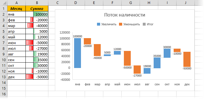
Каскадная диаграмма
Другая интересная форма диаграммы – иерархическая. Прямоугольное поле разбито на ячейки в соответствии с процентной долей той или иной величины в общей сумме значений. Эта форма предназначена для визуализации, наглядного сравнения разных составных частей процесса или явления.
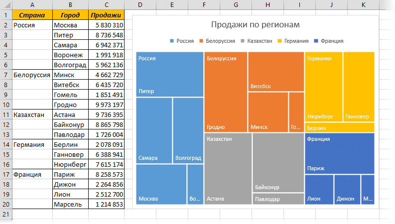
Иерархическая диаграмма
Усовершенствованная круговая диаграмма называется «солнечные лучи». Данные для этой диграммы берутся из трех столбцов: название группф, название подгруппы и числовая характеристика.
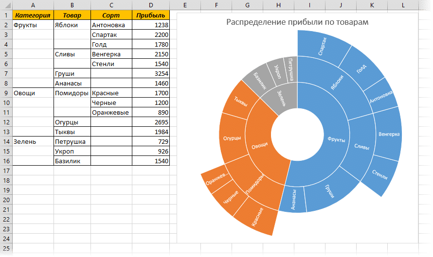
Диаграмма «Солнечные лучи»
Следующая новинка – диаграмма Парето. Это не только визуализация для наглядности, но и статистический анализ данных в Excel 2016. Данные проиндексированы, то есть расположены в порядке убывания. Линией обозначена функция распределения.
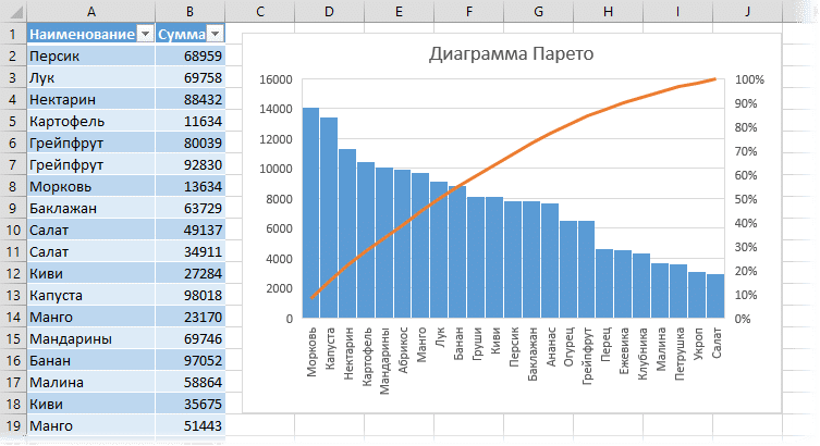
Диаграмма Парето
Еще одна востребованная диаграмма – частотная. Данные разбиты на интервалы, и каждому интервалу соответствует количество элементов с зарактеристиками, попадающими в этот интервал.
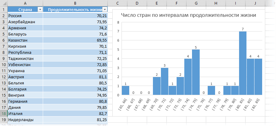
Частотная диаграмма
Приведенный перечень не охватывает всей информации о том, как происходит анализ данных в Excеl 2016. В программе имеется надстройки, в частности Пакет анализа, с содержащий как старые усовершенствованный опции, так и новые. Все тонкости работы с новой версией станут известны, когда в продажу поступит не тестовая, а окончательная версия программы.