
Summary:
Does merging rows and columns in Excel seems a tough task for you to perform? Read this tutorial to learn different ways to merge rows and columns in Excel.
Microsoft Excel is a very useful application and can be used for performing various tasks. This is the reason Excel provides various useful functions to make the task easy for the users.
One of the most common tasks that everyone needs performing now and then is merging rows and columns.
But the problem is that performing this is not an easy task and Excel does not provide any tool to do this.
This is quite complicated as merging rows and columns in some cases causes data loss.
As while trying to combine two or more rows in the worksheet by making use of the Merge & Center button (Home tab > Alignment group), you will start getting the error message:
“The selection contains multiple data values. Merging into one cell will keep the upper-left most data only.”

And if you click OK, merged cells would contain just the value of the top-left cell and as a result, entire other data will be removed.
So this is what leads you to Panic situation!!!
To get rid of this, today in this article I am sharing different ways to easily merge rows and columns in excel without losing any data.
Below check out the fixes on how to merge rows in Excel or how to merge columns in Excel.
To recover Excel data without any data loss, we recommend this tool:
This software will prevent Excel workbook data such as BI data, financial reports & other analytical information from corruption and data loss. With this software you can rebuild corrupt Excel files and restore every single visual representation & dataset to its original, intact state in 3 easy steps:
- Download Excel File Repair Tool rated Excellent by Softpedia, Softonic & CNET.
- Select the corrupt Excel file (XLS, XLSX) & click Repair to initiate the repair process.
- Preview the repaired files and click Save File to save the files at desired location.
There are different methods for combining row and columns text in Excel. Here check the ways one by one to merge data without losing it. First, check how to merge rows in Excel.
Part 1# How To Merge Rows in Excel
When it comes to merging the Excel rows there are two ways that allow you to merge rows data easily.
- Merge Excel rows using a formula
- Combine multiple rows using the Merge Cells add-in
1. How to Merge Multiple Rows using Excel Formulas
Excel provides various formulas that help you combine data from different rows. Possibly the easiest one is the CONCATENATE function. So here checks out some examples for concatenating numerous rows into one:
- Merge rows with spaces between data: For example =CONCATENATE(B1,” “,B2,” “,B3)
- Combine rows without any space between the values: For example =CONCATENATE(A1,A2,A3)
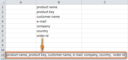
- Merge rows > separate the values with comma: For Example =CONCATENATE(A1,”, “,A2,”, “,A3)
Now check how the CONCATENATE formula works on the real data.

- On the sheet choose an empty cell and type the formula into it. Type the formula as per the data rows
- And copy the formula across entire other cells in the row.

- Now, simply you are having several data rows merged into one row.
2. How to Combine Rows in Excel using the Merge Cells Add-in

The Merge Cells add-in is used for merging various types of cells in Excel. This allows you to merges the individual cells and also combines data from entire rows or columns.
Please Note: You need to download a merge cell add-ins for third-party sites available online. Search in Google for add-ins.
Follow the given steps to combine two or more rows in your table:
- Choose rows you are looking to merge > click on the Merge Cells icon.
- Now the merge cells dialog window opens with a table or range selected already. And in the upper part of the window, you can see the three basic things:

-
- How you want to join cells – For combining rows of data > choose “column by column“.
- How to separate merged values with – an array of standard separators is available to choose from > comma, space, semicolon, and a line break. So select the separator as per your desire.
- Where you need to place the merged cells > either the top cell or bottom cell.
- Now check the lower part of the Windows to check if you need any additional options:

-
- Clear the content of selected cells – Choose this if need data to remain in the merged cells only.
- Merge all areas in the selection – This option allows you to merge rows in two or more non-adjacent ranges.
- Skip empty cells and Wrap text – Well, these are self-explanatory.
- Lastly, Create a backup copy of the worksheet – This option is checked by default. It is just a precaution that keeps you on the safe side and prevents the risk of data loss.
- Click the Merge button > to check the result – possible the merged rows of data separated by line breaks.
So, these are the two ways that allow you to merge rows in Excel without any data loss. Now, check out the ways on how to combine two columns in Excel.
Part 2# How To Merge Columns In Excel

Here check out the 3 ways to merge data from several columns into one without using VBA macro.
- Merge two columns using formulas
- Combine columns data via NotePad
- The fastest way to join multiple columns
1. Merge Two Columns using Excel Formulas
1. Into your table > insert a new column > in the column header place the mouse pointer > right-click the mouse > select Insert from the context menu. Name the newly added columns for eg. – “Full Name”

2. In the cell D2, write the formula: =CONCATENATE(B2,” “,C2). The B2 and C2 are the addresses of First Name and Last Name. And in the formula, the quotation marks “” is the separator that will be inserted between merged names any other symbol can be used as a separator e.g. a comma.

3. Just like this, join data from several cells into one by making use of any separator of your choice.

4. Simply, copy the formula to other cells of the Full Name column. If the First name or the Last name is deleted, then the corresponding data in the Full name Column will also be gone.

5. Next, try converting the formula to a value so that you can remove the unnecessary columns from the Excel worksheet. Choose entire cells with data in the merged column (choose the first cell in “Full Name” Column > press Ctrl +Shift + Arrow Down)
6. Now copy the contents of the columns to clipboard > right click on the cell in the same column (“Full Name”) > choose “Paste Special” context menu > choose “Values” radio button > click OK.

7. Now remove “First Name” & “Last Name” columns that are not required. Click the column B header > press and hold Ctrl > click column C header.

8. After that make a right-click on any selected columns > select Delete from the context menu.
9. This is it, now you have successfully merged the names from 2 columns into one.

2. Combine columns Data via Notepad
This is another way that allows you to merge several columns. Here you don’t need any formulas. This is suitable for combining adjacent columns to make use of the same delimiter for all of them.
For Example: If looking for combining 2 columns with First Names and Last Names into one:
- Choose both columns you need to merge: Click B1 > press Shift + ArrrowRight for choosing C1 > then hit Ctrl + Shift + ArrowDown for choosing entire data cells with data in two columns.

- And copy data to clipboard > open Notepad > insert data from the clipboard to the Notepad

- Then copy tab character to clipboard > hit Tab right in Notepad > hit Ctrl + Shift + LeftArrow > press Ctrl + X.
- After that Replace Tab characters in Notepad with the separator, you require.
- Hit Ctrl + H for opening the “Replace” dialog box > paste the Tab character from the clipboard in Find what field > type the separator Space, comma etc in “Replace with” field. Hit the Replace All button > to close the dialog box press Cancel

- Now select the entire text in the Notepad and copy it to Clipboard.
- Then switch back to Excel worksheet (press Alt + Tab) > choose B1 cell and paste text from Clipboard to your table.

- And rename column B to “Full Name“ and remove the “Last name” column.
So, this is the second way that allows you to merge columns in Excel without any data loss.
3. Join Columns Using Merge Cells Add-in For Excel
This is the easiest and quickest way for combining data from numerous Excel columns into one. Just make use of the third party merge cells add-in for Excel.
And with the merge cells add-in you can merge data from many cells by using any separator you like (for example carriage return or line break). With this, you can join row by row, column by column, or merge data from the selected cell into one without any loss.
There are many third-party add-ins online sites that allow you to download the add-ins and merge the cells easily in just a few clicks.
Conclusion:
So this is all about merging rows and columns in Excel without any data loss.
Follow the given steps to combine text in rows and columns easily.
Hope the given different steps will allow you to perform the task easily in the rows and column. Here I have described different methods of merging rows and columns data in Excel without any data loss.
So make use of anyone that you find easy for you.
However if in case you come to face any issue or data loss situation in Excel then make use of the MS Excel Repair Tool. This is the best tool that allows you to repair and recover data from the corrupted, damaged Excel file.
Additionally, you can learn advanced Excel to become more productive and easily utilize Excel functions and formulas.

Priyanka is an entrepreneur & content marketing expert. She writes tech blogs and has expertise in MS Office, Excel, and other tech subjects. Her distinctive art of presenting tech information in the easy-to-understand language is very impressive. When not writing, she loves unplanned travels.
Merge and unmerge cells
You can’t split an individual cell, but you can make it appear as if a cell has been split by merging the cells above it.

Merge cells
-
Select the cells to merge.
-
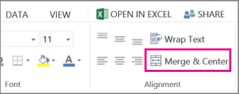
Select Merge & Center.
Important: When you merge multiple cells, the contents of only one cell (the upper-left cell for left-to-right languages, or the upper-right cell for right-to-left languages) appear in the merged cell. The contents of the other cells that you merge are deleted.
Unmerge cells
-
Select the Merge & Center down arrow.
-
Select Unmerge Cells.
Important:
-
You cannot split an unmerged cell. If you are looking for information about how to split the contents of an unmerged cell across multiple cells, see Distribute the contents of a cell into adjacent columns.
-
After merging cells, you can split a merged cell into separate cells again. If you don’t remember where you have merged cells, you can use the Find command to quickly locate merged cells.
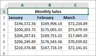
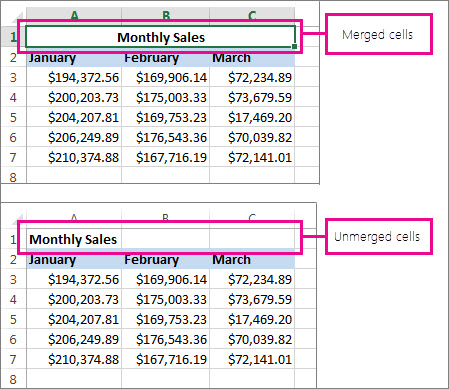
Merging combines two or more cells to create a new, larger cell. This is a great way to create a label that spans several columns.
In the example here, cells A1, B1, and C1 were merged to create the label “Monthly Sales” to describe the information in rows 2 through 7.
Merge cells
Merge two or more cells by following these steps:
-
Select two or more adjacent cells you want to merge.
Important: Ensure that the data you want to retain is in the upper-left cell, and keep in mind that all data in the other merged cells will be deleted. To retain any data from those other cells, simply copy it to another place in the worksheet—before you merge.
-
On the Home tab, select Merge & Center.


Tips:
-
If Merge & Center is disabled, ensure that you’re not editing a cell—and the cells you want to merge aren’t formatted as an Excel table. Cells formatted as a table typically display alternating shaded rows, and perhaps filter arrows on the column headings.
-
To merge cells without centering, click the arrow next to Merge and Center, and then click Merge Across or Merge Cells.
Unmerge cells
If you need to reverse a cell merge, click onto the merged cell and then choose Unmerge Cells item in the Merge & Center menu (see the figure above).
Split text from one cell into multiple cells
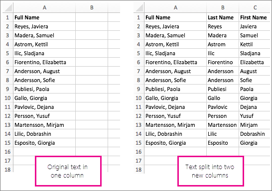
You can take the text in one or more cells, and distribute it to multiple cells. This is the opposite of concatenation, in which you combine text from two or more cells into one cell.
For example, you can split a column containing full names into separate First Name and Last Name columns:
Follow the steps below to split text into multiple columns:
-
Select the cell or column that contains the text you want to split.
-
Note: Select as many rows as you want, but no more than one column. Also, ensure that are sufficient empty columns to the right—so that none of your data is deleted. Simply add empty columns, if necessary.
-
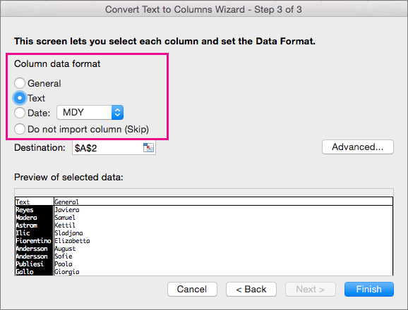
Click Data >Text to Columns, which displays the Convert Text to Columns Wizard.
-
Click Delimited > Next.
-
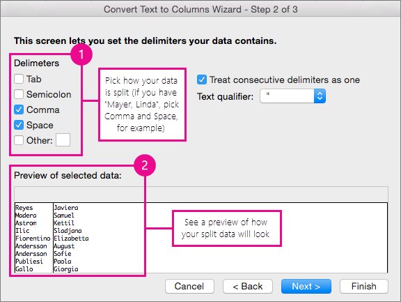
Check the Space box, and clear the rest of the boxes. Or, check both the Comma and Space boxes if that is how your text is split (such as «Reyes, Javiers», with a comma and space between the names). A preview of the data appears in the panel at the bottom of the popup window.
-
Click Next and then choose the format for your new columns. If you don’t want the default format, choose a format such as Text, then click the second column of data in the Data preview window, and click the same format again. Repeat this for all of the columns in the preview window.
-
Click the
button to the right of the Destination box to collapse the popup window. -
Anywhere in your workbook, select the cells that you want to contain the split data. For example, if you are dividing a full name into a first name column and a last name column, select the appropriate number of cells in two adjacent columns.
-
Click the
button to expand the popup window again, and then click the Finish button.
 button to the right of the Destination box to collapse the popup window.
 button to expand the popup window again, and then click the Finish button.
Merging combines two or more cells to create a new, larger cell. This is a great way to create a label that spans several columns. For example, here cells A1, B1, and C1 were merged to create the label “Monthly Sales” to describe the information in rows 2 through 7.
Merge cells
-
Click the first cell and press Shift while you click the last cell in the range you want to merge.
Important: Make sure only one of the cells in the range has data.
-
Click Home > Merge & Center.
If Merge & Center is dimmed, make sure you’re not editing a cell or the cells you want to merge aren’t inside a table.
Tip: To merge cells without centering the data, click the merged cell and then click the left, center or right alignment options next to Merge & Center.
If you change your mind, you can always undo the merge by clicking the merged cell and clicking Merge & Center.
Unmerge cells
To unmerge cells immediately after merging them, press Ctrl + Z. Otherwise do this:
-
Click the merged cell and click Home > Merge & Center.
The data in the merged cell moves to the left cell when the cells split.
Need more help?
You can always ask an expert in the Excel Tech Community or get support in the Answers community.
See Also
Overview of formulas in Excel
How to avoid broken formulas
Find and correct errors in formulas
Excel keyboard shortcuts and function keys
Excel functions (alphabetical)
Excel functions (by category)
Need more help?
Last Update: Jan 03, 2023
This is a question our experts keep getting from time to time. Now, we have got the complete detailed explanation and answer for everyone, who is interested!
Asked by: Rosa Jacobi
Score: 4.9/5
(52 votes)
How to merge cells
- Highlight the cells you want to merge.
- Click on the arrow just next to «Merge and Center.»
- Scroll down to click on «Merge Cells». This will merge both rows and columns into one large cell, with alignment intact. …
- This will merge the content of the upper-left cell across all highlighted cells.
How do I combine data from multiple rows into one in Excel?
Merge Excel rows using a formula. Combine multiple rows with Merge Cells add-in.
…
To merge two or more rows into one, here’s what you need to do:
- Select the range of cells where you want to merge rows.
- Go to the Ablebits Data tab > Merge group, click the Merge Cells arrow, and then click Merge Rows into One.
How do I merge rows but not columns?
Select the range of cells containing the values you need to merge, and expand the selection to the right blank column to output the final merged values. Then click Kutools > Merge & Split > Combine Rows, Columns or Cells withut Losing Data. 2.
How do I merge cells in each row?
Merge cells
- Select the cells that you want to merge.
- Under Table Tools, on the Layout tab, in the Merge group, click Merge Cells.
How do you merge cells but keep all data?
How to merge cells in Excel without losing data
- Select all the cells you want to combine.
- Make the column wide enough to fit the contents of all cells.
- On the Home tab, in the Editing group, click Fill > Justify. …
- Click Merge and Center or Merge Cells, depending on whether you want the merged text to be centered or not.
26 related questions found
How do I combine Data from multiple cells into one cell in Excel?
Combine data with the Ampersand symbol (&)
- Select the cell where you want to put the combined data.
- Type = and select the first cell you want to combine.
- Type & and use quotation marks with a space enclosed.
- Select the next cell you want to combine and press enter. An example formula might be =A2&» «&B2.
How do I consolidate Data in Excel?
Click Data>Consolidate (in the Data Tools group). In the Function box, click the summary function that you want Excel to use to consolidate the data. The default function is SUM. Select your data.
How do you copy multiple rows in one row in Excel?
To include multiple consecutive rows, click on the top row’s number, hold down the Shift key and then click on the bottom row number to highlight all of the rows in between. To include multiple non-consecutive rows, hold down the Ctrl key and then click on each row number you’d like to copy.
How do I consolidate and sum data in Excel?
Combine duplicate rows and sum the values with Consolidate function
- Click a cell where you want to locate the result in your current worksheet.
- Go to click Data > Consolidate, see screenshot:
- In the Consolidate dialog box:
- After finishing the settings, click OK, and the duplicates are combined and summed.
How do you combine duplicate rows and sum the values in sheets?
Combine duplicate rows in Google Sheets
- Start Combine Duplicate Rows.
- Step 1: Select your data.
- Step 2: Identify key columns.
- Step 3: Choose columns with the values to merge.
- Get the result.
How do I sum values based on criteria in another column in Excel?
(1) Select the column name that you will sum based on, and then click the Primary Key button; (2) Select the column name that you will sum, and then click the Calculate > Sum. (3) Click the Ok button.
What is Sumproduct function in Excel?
The SUMPRODUCT function returns the sum of the products of corresponding ranges or arrays. The default operation is multiplication, but addition, subtraction, and division are also possible.
What is the difference between Sumif and SUMPRODUCT?
SUMPRODUCT is more mathematical calculation-based. SUMIFS is more logic-based. SUMPRODUCT can be used to find the sum of products as well as conditional sums. … SUMIFS can only find conditional sums.
Is SUMPRODUCT faster than Sumifs?
In fact, it turns out that the SUMIFS approach is 15 times faster than the SUMPRODUCT one at coming up with the answer on this mammoth dataset.
How do you Sumif two conditions in Excel?
As SUMIFS function by default entertains multiple criteria based on AND logic, but to sum numbers based on multiple criteria using OR logic, you need to SUMIFS function within an array constant. Remember, you cannot use an expression or cell reference an array constant.
How do I sum duplicates in Google Sheets?
With Power Tools, all it takes is to open the Data group, click Combine Duplicate Rows, and follow 3 steps:
- Select your data.
- Select key columns with duplicates.
- Choose how to bring uniques to one row: calculate the numbers or merge values that refer to the same record.
How do I combine duplicate rows into one keeping unique values?
How to merge duplicate rows in Excel
- On Step 1 select your range.
- On Step 2 choose the key columns with duplicate records.
- On Step 3 indicate the columns with the values to merge and choose demiliters.
- All the duplicates are merged according to the key columns.
How do I merge rows and values in Google Sheets?
- On your computer, open a spreadsheet in Google Sheets.
- Select the rows, columns, or cells to merge.
- At the top, click Format. Merge cells, then select how you want your cells to be merged.
How do I convert multiple row data to single row?
In the Combine Columns or Rows dialog box, select Combine into single cell in the first section, then specify a separator, and finally click the OK button. Now all selected cells in different rows are combined into one cell immediately.
How do you copy multiple cells in Excel without dragging?
Instead, you can accomplish the same copy with a double-click instead of a drag. Set up your formula in the top cell, position the mouse in the lower right-hand corner of the cell until you see the plus, and double-click. Note that this option can copy the formula down as far as Excel finds data to the left.
How do you copy multiple selections in Excel?
#1 go to HOME tab, click drop-down arrow in the Clipboard group. and the Clipboard pane will open. #2 copy the selected ranges or non adjacent range of cells that you want to copy via press CTRL +C keys. #3 select one destination cell to place the data.
Depending how you want to format a body of text in Microsoft Excel, you will sometimes have to merge cells. Whatever your reason is, there are a few different techniques you can use. These can help you to achieve the merging of cells, rows, and columns. Some methods will get rid of some of the data in cells, so you have to decide how you want the final result to look beforehand.
Merging Cells
You will find the built-in merge options under the Home tab of Microsoft Excel.

The merge options available are:
- Merge & Center: This option merges cells into one and centers the text. However, only the text from the leftmost cell is kept.
- Merge Across: This option merges cells across from each other into one. All of the rows in a selection chosen to be merged are separated. However, only the text in the leftmost cell of each row is kept.
- Merge Cells: This merges all of the cells in a selection into one. The text is not centered, and only the text from the leftmost cell is kept.
- Unmerge
Consider a case where you made a selection that made up six rows and two columns.

If you choose “Merge & Center,” the result will be centered in the area you selected.

On the other hand, if you choose “Merge Across,” the text in the left cells of the rows that were selected will be kept.

With the “Merge Cells” option, the text in the leftmost cell of the selection is kept and the cells are all fused. The text is not centered in this case.

Merging Rows
If you want to merge rows, then the CONCATENATE function is your best bet. If you wanted to merge a series of rows together into one row where the text is separated by commas, you can use the following formula in a blank cell:

=CONCATENATE(A2,", ",A2,", ",A3,", ",A4,", ",A5,", ",A6...)
The extra commas and quotation marks are included so that there is a space after the comma that comes after each word in the list.

The CONCATENATE function is your friend again when it comes to merging columns. In order to merge a group of columns together, you have to pick out the relevant cells in the columns you want to fuse and include them in your CONCATENATE formula. For example, if you had column H and column I with three items in each column, the following formula could be used to merge items together:
=CONCATENATE(H1,", ",H2,", ",H3,", ",I1,", ",I2,", ",I3)
An Aside About the Concatenate Function
If you want to have your merged content without spaces, then use the concatenate function like this:
=CONCATENATE(A2,A2,A3,A4,A5,A6)

On the other hand, if you want to have your merged content with spaces, you can use the concatenate function like this:
=CONCATENATE(A2," ",A2," ",A3," ",A4," ",A5," ",A6)

This applies to the merging of both rows and columns.
Wrapping Up
Depending on what you’re doing, you’ll need to format your data differently. This makes merging cells, rows, and columns an invaluable tool. We have covered different techniques here. Feel free to get creative about how you use them. We’ve covered the basics here, but you can do different things like changing up the spacing of your merged content to your preferences. We can also show you how to make your Excel workbook read-only.

William Elcock
William has been fiddling with tech for as long as he remembers. This naturally transitioned into helping friends with their tech problems and then into tech blogging.
Subscribe to our newsletter!
Our latest tutorials delivered straight to your inbox
To the immediate right of the end of your last column, at the first row, type the following:
=A1 & "-" & B1
Go one column over to the right and type this:
=A2 & "-" & B2
Now highlight both of those new cells that you just typed, and grab the little autofill box in the lower right corner of your selected cells, and drag over until your new area is the same width as the original row.
Now, highlight the entire new section you’ve just created, and drag it down to the bottom of your data area.
Highlight the whole block of new data, hit Ctrl-C, and then right click somwhere and choose «Paste Special». In the dialog that appears, choose «Values», and hit «OK». Now you can move this new block anywhere you want without regard to other cells.
Finally, you will need to delete every other row of your newly pasted data, beginning with the second row.