
I have Excel files with multiple sheets, each of which looks a little like this (but much longer):
        Sample  CD4     CD8
Day 1   8311    17.3    6.44
        8312    13.6    3.50
        8321    19.8    5.88
        8322    13.5    4.09
Day 2   8311    16.0    4.92
        8312    5.67    2.28
        8321    13.0    4.34
        8322    10.6    1.95
The first column is actually four cells merged vertically.
When I read this using pandas.read_excel, I get a DataFrame that looks like this:
       Sample    CD4   CD8
Day 1    8311  17.30  6.44
NaN      8312  13.60  3.50
NaN      8321  19.80  5.88
NaN      8322  13.50  4.09
Day 2    8311  16.00  4.92
NaN      8312   5.67  2.28
NaN      8321  13.00  4.34
NaN      8322  10.60  1.95
How can I either get Pandas to understand merged cells, or quickly and easily remove the NaN and group by the appropriate value? (One approach would be to reset the index, step through to find the values and replace NaNs with values, pass in the list of days, then set the index to the column. But it seems like there should be a simpler approach.)
When you read an Excel file with merged cells into a pandas DataFrame, the merged cells will automatically be filled with NaN values.
The easiest way to fill in these NaN values after importing the file is to use the pandas fillna() function as follows:
df = df.fillna(method='ffill', axis=0)
The following example shows how to use this syntax in practice.
Suppose we have the following Excel file called merged_data.xlsx that contains information about various basketball players:

Notice that the values in the Team column are merged.
Players A through D belong to the Mavericks while players E through H belong to the Rockets.
Suppose we use the read_excel() function to read this Excel file into a pandas DataFrame:
import pandas as pd

#import Excel fie
df = pd.read_excel('merged_data.xlsx')

#view DataFrame
print(df)

        Team Player  Points  Assists
0  Mavericks      A      22        4
1        NaN      B      29        4
2        NaN      C      45        3
3        NaN      D      30        7
4    Rockets      E      29        8
5        NaN      F      16        6
6        NaN      G      25        9
7        NaN      H      20       12
By default, pandas fills in the merged cells with NaN values.
To fill in each of these NaN values with the team names instead, we can use the fillna() function as follows:
#fill in NaN values with team names
df = df.fillna(method='ffill', axis=0)

#view updated DataFrame
print(df)

        Team Player  Points  Assists
0  Mavericks      A      22        4
1  Mavericks      B      29        4
2  Mavericks      C      45        3
3  Mavericks      D      30        7
4    Rockets      E      29        8
5    Rockets      F      16        6
6    Rockets      G      25        9
7    Rockets      H      20       12
Notice that each of the NaN values has been filled in with the appropriate team name.
Note that the argument axis=0 tells pandas to fill in the NaN values vertically.
To instead fill in NaN values horizontally across columns, you can specify axis=1.
Note: You can find the complete documentation for the pandas fillna() function here.
Additional Resources
The following tutorials explain how to perform other common tasks in pandas:
Pandas: How to Skip Rows when Reading Excel File
Pandas: How to Specify dtypes when Importing Excel File
Pandas: How to Combine Multiple Excel Sheets
In this tutorial, you’ll learn how to save your Pandas DataFrame or DataFrames to Excel files. Being able to save data to this ubiquitous data format is an important skill in many organizations. In this tutorial, you’ll learn how to save a simple DataFrame to Excel, but also how to customize your options to create the report you want!
By the end of this tutorial, you’ll have learned:
- How to save a Pandas DataFrame to Excel
- How to customize the sheet name of your DataFrame in Excel
- How to customize the index and column names when writing to Excel
- How to write multiple DataFrames to Excel in Pandas
- Whether to merge cells or freeze panes when writing to Excel in Pandas
- How to format missing values and infinity values when writing Pandas to Excel
Let’s get started!
The Quick Answer: Use Pandas to_excel
To write a Pandas DataFrame to an Excel file, you can apply the .to_excel() method to the DataFrame, as shown below:
# Saving a Pandas DataFrame to an Excel File
# Without a Sheet Name
df.to_excel(file_name)

# With a Sheet Name
df.to_excel(file_name, sheet_name='My Sheet')

# Without an Index
df.to_excel(file_name, index=False)
Understanding the Pandas to_excel Function
Before diving into any specifics, let’s take a look at the different parameters that the method offers. The method provides a ton of different options, allowing you to customize the output of your DataFrame in many different ways. Let’s take a look:
# The many parameters of the .to_excel() function
df.to_excel(excel_writer, sheet_name='Sheet1', na_rep='', float_format=None, columns=None, header=True, index=True, index_label=None, startrow=0, startcol=0, engine=None, merge_cells=True, encoding=None, inf_rep='inf', verbose=True, freeze_panes=None, storage_options=None)
Let’s break down what each of these parameters does:
| Parameter | Description | Available Options |
|---|---|---|
excel_writer= |
The path of the ExcelWriter to use | path-like, file-like, or ExcelWriter object |
sheet_name= |
The name of the sheet to use | String representing name, default ‘Sheet1’ |
na_rep= |
How to represent missing data | String, default '' |
float_format= |
Allows you to pass in a format string to format floating point values | String |
columns= |
The columns to use when writing to the file | List of strings. If blank, all will be written |
header= |
Accepts either a boolean or a list of values. If a boolean, will either include the header or not. If a list of values is provided, aliases will be used for the column names. | Boolean or list of values |
index= |
Whether to include an index column or not. | Boolean |
index_label= |
Column labels to use for the index. | String or list of strings. |
startrow= |
The upper left cell to start the DataFrame on. | Integer, default 0 |
startcol= |
The upper left column to start the DataFrame on | Integer, default 0 |
engine= |
The engine to use to write. | openpyxl or xlsxwriter |
merge_cells= |
Whether to write multi-index cells or hierarchical rows as merged cells | Boolean, default True |
encoding= |
The encoding of the resulting file. | String |
inf_rep= |
How to represent infinity values (as Excel doesn’t have a representation) | String, default 'inf' |
verbose= |
Whether to display more information in the error logs. | Boolean, default True |
freeze_panes= |
Allows you to pass in a tuple of the row, column to start freezing panes on | Tuple of integers with length 2 |
storage_options= |
Extra options that allow you to save to a particular storage connection | Dictionary |
.to_excel() methodHow to Save a Pandas DataFrame to Excel
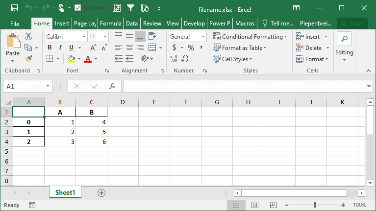
The easiest way to save a Pandas DataFrame to an Excel file is by passing a path to the .to_excel() method. This will save the DataFrame to an Excel file at that path, overwriting an Excel file if it exists already.
Let’s take a look at how this works:
# Saving a Pandas DataFrame to an Excel File
import pandas as pd
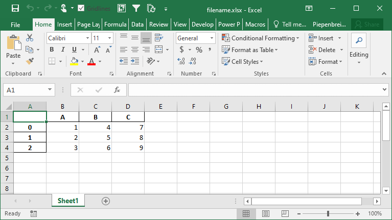
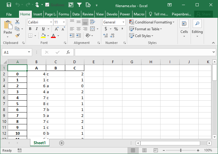
df = pd.DataFrame.from_dict(
{'A': [1, 2, 3], 'B': [4, 5, 6], 'C': [7, 8, 9]}
)
df.to_excel('filename.xlsx')Running the code as shown above will save the file with all other default parameters. This returns the following image:
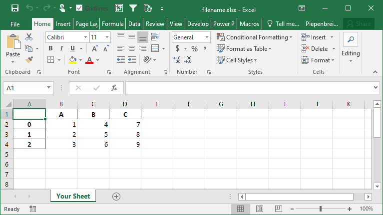
You can specify a sheetname by using the sheet_name= parameter. By default, Pandas will use 'sheet1'.
# Specifying a Sheet Name When Saving to Excel
import pandas as pd
df = pd.DataFrame.from_dict(
    {'A': [1, 2, 3], 'B': [4, 5, 6], 'C': [7, 8, 9]}
)

df.to_excel('filename.xlsx', sheet_name='Your Sheet')
This returns the following workbook:
In the following section, you’ll learn how to customize whether to include an index column or not.
How to Include an Index when Saving a Pandas DataFrame to Excel
By default, Pandas will include the index when saving a Pandas Dataframe to an Excel file. This can be helpful when the index is a meaningful index (such as a date and time). However, in many cases, the index will simply represent the values from 0 through to the end of the records.
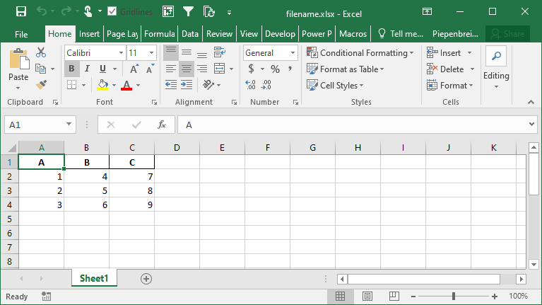
If you don’t want to include the index in your Excel file, you can use the index= parameter, as shown below:
# How to exclude the index when saving a DataFrame to Excel
import pandas as pd
df = pd.DataFrame.from_dict(
    {'A': [1, 2, 3], 'B': [4, 5, 6], 'C': [7, 8, 9]}
)

df.to_excel('filename.xlsx', index=False)
This returns the following Excel file:
In the following section, you’ll learn how to rename an index when saving a Pandas DataFrame to an Excel file.
How to Rename an Index when Saving a Pandas DataFrame to Excel
By default, Pandas will not named the index of your DataFrame. This, however, can be confusing and can lead to poorer results when trying to manipulate the data in Excel, either by filtering or by pivoting the data. Because of this, it can be helpful to provide a name or names for your indices.
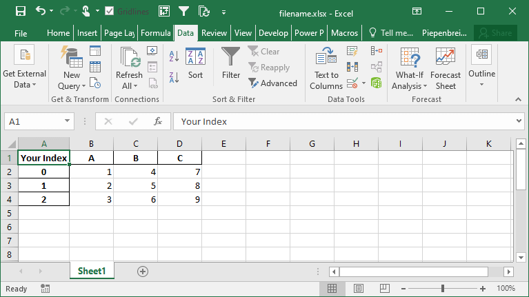
Pandas makes this easy by using the index_label= parameter. This parameter accepts either a single string (for a single index) or a list of strings (for a multi-index). Check out below how you can use this parameter:
# Providing a name for your Pandas index
import pandas as pd
df = pd.DataFrame.from_dict(
    {'A': [1, 2, 3], 'B': [4, 5, 6], 'C': [7, 8, 9]}
)

df.to_excel('filename.xlsx', index_label='Your Index')
This returns the following sheet:
How to Save Multiple DataFrames to Different Sheets in Excel
One of the tasks you may encounter quite frequently is the need to save multi Pandas DataFrames to the same Excel file, but in different sheets. This is where Pandas makes it a less intuitive. If you were to simply write the following code, the second command would overwrite the first command:
# The wrong way to save multiple DataFrames to the same workbook
import pandas as pd
df = pd.DataFrame.from_dict(
    {'A': [1, 2, 3], 'B': [4, 5, 6], 'C': [7, 8, 9]}
)

df.to_excel('filename.xlsx', sheet_name='Sheet1')
df.to_excel('filename.xlsx', sheet_name='Sheet2')
Instead, we need to use a Pandas Excel Writer to manage opening and saving our workbook. This can be done easily by using a context manager, as shown below:
# The Correct Way to Save Multiple DataFrames to the Same Workbook
import pandas as pd
df = pd.DataFrame.from_dict(
    {'A': [1, 2, 3], 'B': [4, 5, 6], 'C': [7, 8, 9]}
)

with pd.ExcelWriter('filename.xlsx') as writer:
    df.to_excel(writer, sheet_name='Sheet1')
    df.to_excel(writer, sheet_name='Sheet2')
This will create multiple sheets in the same workbook. The sheets will be created in the same order as you specify them in the command above.
This returns the following workbook:

How to Save Only Some Columns when Exporting Pandas DataFrames to Excel
When saving a Pandas DataFrame to an Excel file, you may not always want to save every single column. In many cases, the Excel file will be used for reporting and it may be redundant to save every column. Because of this, you can use the columns= parameter to accomplish this.
Let’s see how we can save only a number of columns from our dataset:
# Saving Only a Subset of Columns to Excel
import pandas as pd
df = pd.DataFrame.from_dict(
    {'A': [1, 2, 3], 'B': [4, 5, 6], 'C': [7, 8, 9]}
)

df.to_excel('filename.xlsx', columns=['A', 'B'])
This returns the following Excel file:
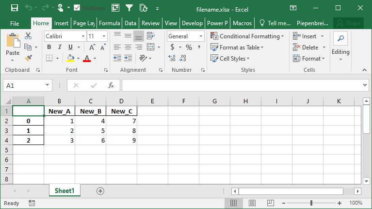
How to Rename Columns when Exporting Pandas DataFrames to Excel
Continuing our discussion about how to handle Pandas DataFrame columns when exporting to Excel, we can also rename our columns in the saved Excel file. The benefit of this is that we can work with aliases in Pandas, which may be easier to write, but then output presentation-ready column names when saving to Excel.
We can accomplish this using the header= parameter. The parameter accepts either a boolean value of a list of values. If a boolean value is passed, you can decide whether to include or a header or not. When a list of strings is provided, then you can modify the column names in the resulting Excel file, as shown below:
# Modifying Column Names when Exporting a Pandas DataFrame to Excel
import pandas as pd
df = pd.DataFrame.from_dict(
    {'A': [1, 2, 3], 'B': [4, 5, 6], 'C': [7, 8, 9]}
)

df.to_excel('filename.xlsx', header=['New_A', 'New_B', 'New_C'])
This returns the following Excel sheet:
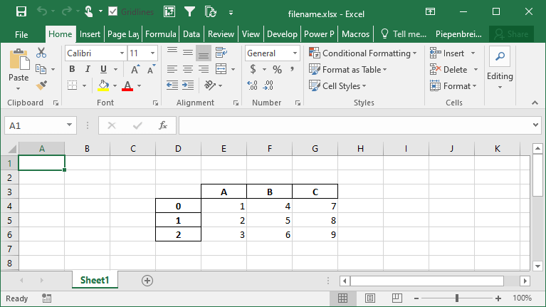
How to Specify Starting Positions when Exporting a Pandas DataFrame to Excel
One of the interesting features that Pandas provides is the ability to modify the starting position of where your DataFrame will be saved on the Excel sheet. This can be helpful if you know you’ll be including different rows above your data or a logo of your company.
Let’s see how we can use the startrow= and startcol= parameters to modify this:
# Changing the Start Row and Column When Saving a DataFrame to an Excel File
import pandas as pd
df = pd.DataFrame.from_dict(
{'A': [1, 2, 3], 'B': [4, 5, 6], 'C': [7, 8, 9]}
)
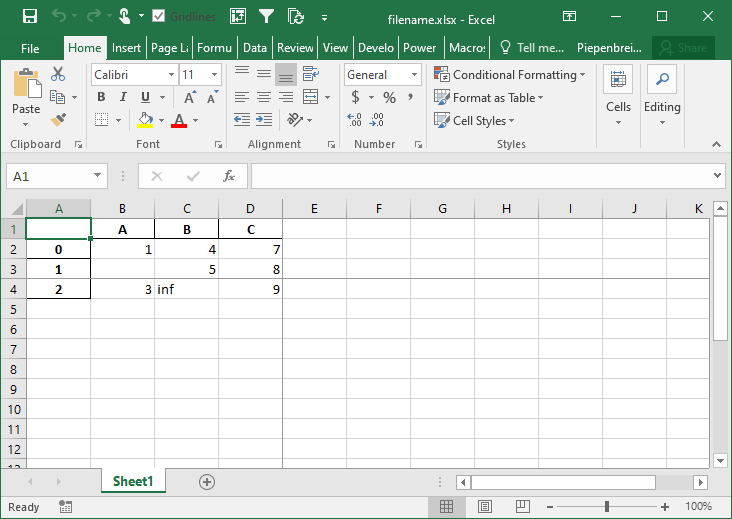
df.to_excel('filename.xlsx', startcol=3, startrow=2)This returns the following worksheet:
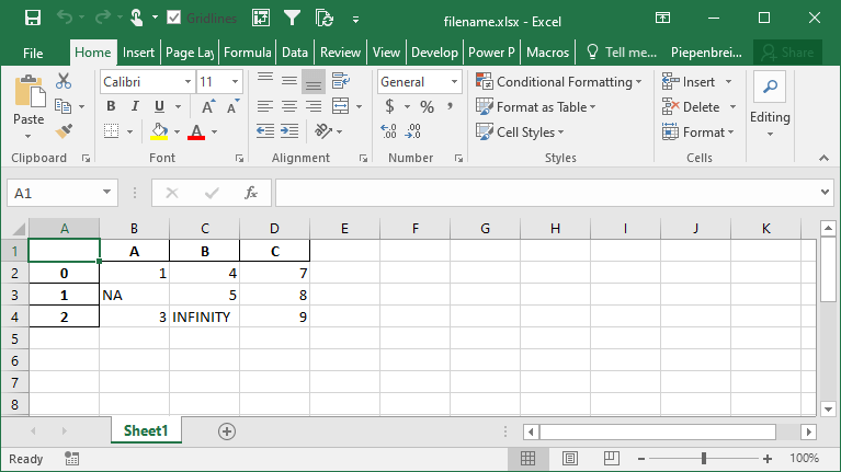
How to Represent Missing and Infinity Values When Saving Pandas DataFrame to Excel
In this section, you’ll learn how to represent missing data and infinity values when saving a Pandas DataFrame to Excel. Because Excel doesn’t have a way to represent infinity, Pandas will default to the string 'inf' to represent any values of infinity.
In order to modify these behaviors, we can use the na_rep= and inf_rep= parameters to modify the missing and infinity values respectively. Let’s see how we can do this by adding some of these values to our DataFrame:
# Customizing Output of Missing and Infinity Values When Saving to Excel
import pandas as pd
import numpy as np

df = pd.DataFrame.from_dict(
    {'A': [1, np.NaN, 3], 'B': [4, 5, np.inf], 'C': [7, 8, 9]}
)

df.to_excel('filename.xlsx', na_rep='NA', inf_rep='INFINITY')
This returns the following worksheet:
How to Merge Cells when Writing Multi-Index DataFrames to Excel
In this section, you’ll learn how to modify the behavior of multi-index DataFrames when saved to Excel. By default Pandas will set the merge_cells= parameter to True, meaning that the cells will be merged. Let’s see what happens when we set this behavior to False, indicating that the cells should not be merged:
# Modifying Merge Cell Behavior for Multi-Index DataFrames
import pandas as pd
import numpy as np
from random import choice

df = pd.DataFrame.from_dict({
    'A': np.random.randint(0, 10, size=50),
    'B': [choice(['a', 'b', 'c']) for i in range(50)],
    'C': np.random.randint(0, 3, size=50)})

pivot = df.pivot_table(index=['B', 'C'], values='A')

pivot.to_excel('filename.xlsx', merge_cells=False)
This returns the Excel worksheet below:
How to Freeze Panes when Saving a Pandas DataFrame to Excel
In this final section, you’ll learn how to freeze panes in your resulting Excel worksheet. This allows you to specify the row and column at which you want Excel to freeze the panes. This can be done using the freeze_panes= parameter. The parameter accepts a tuple of integers (of length 2). The tuple represents the bottommost row and the rightmost column that is to be frozen.
Let’s see how we can use the freeze_panes= parameter to freeze our panes in Excel:
# Freezing Panes in an Excel Workbook Using Pandas
import pandas as pd
import numpy as np

df = pd.DataFrame.from_dict(
    {'A': [1, np.NaN, 3], 'B': [4, 5, np.inf], 'C': [7, 8, 9]}
)

df.to_excel('filename.xlsx', freeze_panes=(3,4))
This returns the following workbook:
Conclusion
In this tutorial, you learned how to save a Pandas DataFrame to an Excel file using the to_excel method. You first explored all of the different parameters that the function had to offer at a high level. Following that, you learned how to use these parameters to gain control over how the resulting Excel file should be saved. For example, you learned how to specify sheet names, index names, and whether to include the index or not. Then you learned how to include only some columns in the resulting file and how to rename the columns of your DataFrame. You also learned how to modify the starting position of the data and how to freeze panes.
Additional Resources
To learn more about related topics, check out the tutorials below:
- How to Use Pandas to Read Excel Files in Python
- Pandas Dataframe to CSV File – Export Using .to_csv()
- Introduction to Pandas for Data Science
- Official Documentation: Pandas to_excel
The worksheet class represents an Excel worksheet. It handles operations such
as writing data to cells or formatting worksheet layout.
A worksheet object isn’t instantiated directly. Instead a new worksheet is
created by calling the add_worksheet() method from a Workbook()
object:
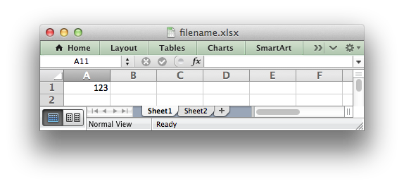
workbook   = xlsxwriter.Workbook('filename.xlsx')

worksheet1 = workbook.add_worksheet()
worksheet2 = workbook.add_worksheet()

worksheet1.write('A1', 123)

workbook.close()
XlsxWriter supports Excels worksheet limits of 1,048,576 rows by 16,384
columns.
worksheet.write()
-
write(row, col, *args) -
Write generic data to a worksheet cell.
Parameters: - row – The cell row (zero indexed).
- col – The cell column (zero indexed).
- *args – The additional args that are passed to the sub methods
such as number, string and cell_format.
Returns: 0: Success.
Returns: -1: Row or column is out of worksheet bounds.
Returns: Other values from the called write methods.
Excel makes a distinction between data types such as strings, numbers, blanks,
formulas and hyperlinks. To simplify the process of writing data to an
XlsxWriter file the write() method acts as a general alias for several
more specific methods:
write_string()write_number()write_blank()write_formula()write_datetime()write_boolean()write_url()
The rules for handling data in write() are as follows:
- Data types
float,int,long,decimal.Decimaland
fractions.Fractionare written usingwrite_number(). - Data types
datetime.datetime,datetime.date
datetime.timeordatetime.timedeltaare written using
write_datetime(). Noneand empty strings""are written usingwrite_blank().- Data type
boolis written usingwrite_boolean().
Strings are then handled as follows:
- Strings that start with
"="are assumed to match a formula and are written
usingwrite_formula(). This can be overridden, see below. - Strings that match supported URL types are written using
write_url(). This can be overridden, see below. - When the
Workbook()constructorstrings_to_numbersoption is
Truestrings that convert to numbers usingfloat()are written
usingwrite_number()in order to avoid Excel warnings about “Numbers
Stored as Text”. See the note below. - Strings that don’t match any of the above criteria are written using
write_string().
If none of the above types are matched the value is evaluated with float()
to see if it corresponds to a user defined float type. If it does then it is
written using write_number().
Finally, if none of these rules are matched then a TypeError exception is
raised. However, it is also possible to handle additional, user defined, data
types using the add_write_handler() method explained below and in
Writing user defined types.
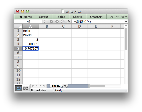
Here are some examples:
worksheet.write(0, 0, 'Hello')          # write_string()
worksheet.write(1, 0, 'World')          # write_string()
worksheet.write(2, 0, 2)                # write_number()
worksheet.write(3, 0, 3.00001)          # write_number()
worksheet.write(4, 0, '=SIN(PI()/4)')   # write_formula()
worksheet.write(5, 0, '')               # write_blank()
worksheet.write(6, 0, None)             # write_blank()
This creates a worksheet like the following:
Note
The Workbook() constructor option takes three optional arguments
that can be used to override string handling in the write() function.
These options are shown below with their default values:
xlsxwriter.Workbook(filename, {'strings_to_numbers':  False,
                               'strings_to_formulas': True,
                               'strings_to_urls':     True})
The write() method supports two forms of notation to designate the position
of cells: Row-column notation and A1 notation:
# These are equivalent.
worksheet.write(0, 0, 'Hello')
worksheet.write('A1', 'Hello')
See Working with Cell Notation for more details.
The cell_format parameter in the sub write methods is used to apply
formatting to the cell. This parameter is optional but when present it should
be a valid Format object:
cell_format = workbook.add_format({'bold': True, 'italic': True})

worksheet.write(0, 0, 'Hello', cell_format)  # Cell is bold and italic.
worksheet.add_write_handler()
-
add_write_handler(user_type, user_function) -
Add a callback function to the
write()method to handle user define
types.Parameters: - user_type (type) – The user
type()to match on. - user_function (types.FunctionType) – The user defined function to write the type data.
- user_type (type) – The user
As explained above, the write() method maps basic Python types to
corresponding Excel types. If you want to write an unsupported type then you
can either avoid write() and map the user type in your code to one of the
more specific write methods or you can extend it using the
add_write_handler() method.
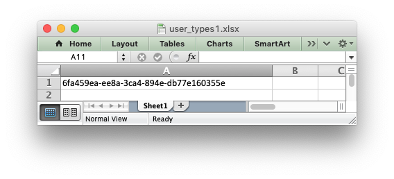
For example, say you wanted to automatically write uuid values as
strings using write() you would start by creating a function that takes the
uuid, converts it to a string and then writes it using write_string():
def write_uuid(worksheet, row, col, uuid, format=None):
    string_uuid = str(uuid)
    return worksheet.write_string(row, col, string_uuid, format)
You could then add a handler that matches the uuid type and calls your
user defined function:
#                           match,     action()
worksheet.add_write_handler(uuid.UUID, write_uuid)
Then you can use write() without further modification:
my_uuid = uuid.uuid3(uuid.NAMESPACE_DNS, 'python.org')

# Write the UUID. This would raise a TypeError without the handler.
worksheet.write('A1', my_uuid)
Multiple callback functions can be added using add_write_handler() but
only one callback action is allowed per type. However, it is valid to use the
same callback function for different types:
worksheet.add_write_handler(int,   test_number_range)
worksheet.add_write_handler(float, test_number_range)
See Writing user defined types for more details on how this feature works and
how to write callback functions, and also the following examples:
- Example: Writing User Defined Types (1)
- Example: Writing User Defined Types (2)
- Example: Writing User Defined types (3)
worksheet.write_string()
-
write_string(row, col, string[, cell_format]) -
Write a string to a worksheet cell.
Parameters: - row (int) – The cell row (zero indexed).
- col (int) – The cell column (zero indexed).
- string (string) – String to write to cell.
- cell_format (Format) – Optional Format object.
Returns: 0: Success.
Returns: -1: Row or column is out of worksheet bounds.
Returns: -2: String truncated to 32k characters.
The write_string() method writes a string to the cell specified by row
and column:
worksheet.write_string(0, 0, 'Your text here')
worksheet.write_string('A2', 'or here')
Both row-column and A1 style notation are supported, as shown above. See
Working with Cell Notation for more details.
The cell_format parameter is used to apply formatting to the cell. This
parameter is optional but when present is should be a valid
Format object.
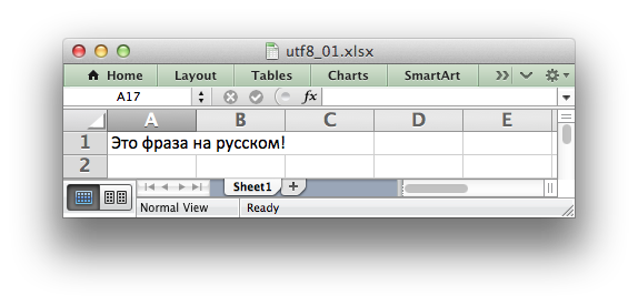
Unicode strings are supported in UTF-8 encoding. This generally requires that
your source file is UTF-8 encoded:
worksheet.write('A1', u'Some UTF-8 text')
See Example: Simple Unicode with Python 3 for a more complete example.
Alternatively, you can read data from an encoded file, convert it to UTF-8
during reading and then write the data to an Excel file. See
Example: Unicode — Polish in UTF-8 and Example: Unicode — Shift JIS.
The maximum string size supported by Excel is 32,767 characters. Strings longer
than this will be truncated by write_string().
Note
Even though Excel allows strings of 32,767 characters it can only
display 1000 in a cell. However, all 32,767 characters are displayed in the
formula bar.
worksheet.write_number()
-
write_number(row, col, number[, cell_format]) -
Write a number to a worksheet cell.
Parameters: - row (int) – The cell row (zero indexed).
- col (int) – The cell column (zero indexed).
- number (int or float) – Number to write to cell.
- cell_format (Format) – Optional Format object.
Returns: 0: Success.
Returns: -1: Row or column is out of worksheet bounds.
The write_number() method writes numeric types to the cell specified by
row and column:
worksheet.write_number(0, 0, 123456)
worksheet.write_number('A2', 2.3451)
Both row-column and A1 style notation are supported, as shown above. See
Working with Cell Notation for more details.
The numeric types supported are float, int, long,
decimal.Decimal and fractions.Fraction or anything that can
be converted via float().
When written to an Excel file numbers are converted to IEEE-754 64-bit
double-precision floating point. This means that, in most cases, the maximum
number of digits that can be stored in Excel without losing precision is 15.
Note
NAN and INF are not supported and will raise a TypeError exception unless
the nan_inf_to_errors Workbook() option is used.
The cell_format parameter is used to apply formatting to the cell. This
parameter is optional but when present is should be a valid
Format object.
worksheet.write_formula()
-
write_formula(row, col, formula[, cell_format[, value]]) -
Write a formula to a worksheet cell.
Parameters: - row (int) – The cell row (zero indexed).
- col (int) – The cell column (zero indexed).
- formula (string) – Formula to write to cell.
- cell_format (Format) – Optional Format object.
- value – Optional result. The value if the formula was calculated.
Returns: 0: Success.
Returns: -1: Row or column is out of worksheet bounds.
The write_formula() method writes a formula or function to the cell
specified by row and column:
worksheet.write_formula(0, 0, '=B3 + B4')
worksheet.write_formula(1, 0, '=SIN(PI()/4)')
worksheet.write_formula(2, 0, '=SUM(B1:B5)')
worksheet.write_formula('A4', '=IF(A3>1,"Yes", "No")')
worksheet.write_formula('A5', '=AVERAGE(1, 2, 3, 4)')
worksheet.write_formula('A6', '=DATEVALUE("1-Jan-2013")')
Both row-column and A1 style notation are supported, as shown above. See
Working with Cell Notation for more details.
Array formulas are also supported:
worksheet.write_formula('A7', '{=SUM(A1:B1*A2:B2)}')
See also the write_array_formula() method below.
The cell_format parameter is used to apply formatting to the cell. This
parameter is optional but when present is should be a valid
Format object.
If required, it is also possible to specify the calculated result of the
formula using the optional value parameter. This is occasionally
necessary when working with non-Excel applications that don’t calculate the
result of the formula:
worksheet.write('A1', '=2+2', num_format, 4)
See Formula Results for more details.
Excel stores formulas in US style formatting regardless of the Locale or
Language of the Excel version:
worksheet.write_formula('A1', '=SUM(1, 2, 3)')    # OK
worksheet.write_formula('A2', '=SOMME(1, 2, 3)')  # French. Error on load.
See Non US Excel functions and syntax for a full explanation.
Excel 2010 and 2013 added functions which weren’t defined in the original file
specification. These functions are referred to as future functions. Examples
of these functions are ACOT, CHISQ.DIST.RT , CONFIDENCE.NORM,
STDEV.P, STDEV.S and WORKDAY.INTL. In XlsxWriter these require a
prefix:
worksheet.write_formula('A1', '=_xlfn.STDEV.S(B1:B10)')
See Formulas added in Excel 2010 and later for a detailed explanation and full list of
functions that are affected.
worksheet.write_array_formula()
-
write_array_formula(first_row, first_col, last_row, last_col, formula[, cell_format[, value]]) -
Write an array formula to a worksheet cell.
Parameters: - first_row (int) – The first row of the range. (All zero indexed.)
- first_col (int) – The first column of the range.
- last_row (int) – The last row of the range.
- last_col (int) – The last col of the range.
- formula (string) – Array formula to write to cell.
- cell_format (Format) – Optional Format object.
- value – Optional result. The value if the formula was calculated.
Returns: 0: Success.
Returns: -1: Row or column is out of worksheet bounds.
The write_array_formula() method writes an array formula to a cell range. In
Excel an array formula is a formula that performs a calculation on a set of
values. It can return a single value or a range of values.
An array formula is indicated by a pair of braces around the formula:
{=SUM(A1:B1*A2:B2)}.
For array formulas that return a range of values you must specify the range
that the return values will be written to:
worksheet.write_array_formula(0, 0, 2, 0, '{=TREND(C1:C3,B1:B3)}')
worksheet.write_array_formula('A1:A3',    '{=TREND(C1:C3,B1:B3)}')
Both row-column and A1 style notation are supported, as shown above. See
Working with Cell Notation for more details.
If the array formula returns a single value then the first_ and last_
parameters should be the same:
worksheet.write_array_formula('A1:A1', '{=SUM(B1:C1*B2:C2)}')
It this case however it is easier to just use the write_formula() or
write() methods:
# Same as above but more concise.
worksheet.write('A1', '{=SUM(B1:C1*B2:C2)}')
worksheet.write_formula('A1', '{=SUM(B1:C1*B2:C2)}')
The cell_format parameter is used to apply formatting to the cell. This
parameter is optional but when present is should be a valid
Format object.
If required, it is also possible to specify the calculated result of the
formula (see discussion of formulas and the value parameter for the
write_formula() method above). However, using this parameter only writes a
single value to the upper left cell in the result array. See
Formula Results for more details.
worksheet.write_dynamic_array_formula()
-
write_dynamic_array_formula(first_row, first_col, last_row, last_col, formula[, cell_format[, value]]) -
Write an array formula to a worksheet cell.
Parameters: - first_row (int) – The first row of the range. (All zero indexed.)
- first_col (int) – The first column of the range.
- last_row (int) – The last row of the range.
- last_col (int) – The last col of the range.
- formula (string) – Array formula to write to cell.
- cell_format (Format) – Optional Format object.
- value – Optional result. The value if the formula was calculated.
Returns: 0: Success.
Returns: -1: Row or column is out of worksheet bounds.
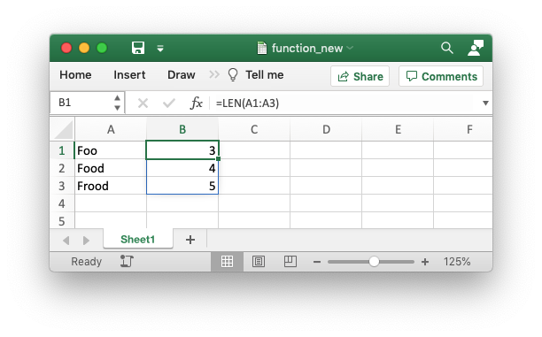
The write_dynamic_array_formula() method writes an dynamic array formula to a cell
range. Dynamic array formulas are explained in detail in Dynamic Array support.
The syntax of write_dynamic_array_formula() is the same as
write_array_formula(), shown above, except that you don’t need to add
{} braces:
worksheet.write_dynamic_array_formula('B1:B3', '=LEN(A1:A3)')
Which gives the following result:
It is also possible to specify the first cell of the range to get the same
results:
worksheet.write_dynamic_array_formula('B1:B1', '=LEN(A1:A3)')
See also Example: Dynamic array formulas.
worksheet.write_blank()
-
write_blank(row, col, blank[, cell_format]) -
Write a blank worksheet cell.
Parameters: - row (int) – The cell row (zero indexed).
- col (int) – The cell column (zero indexed).
- blank – None or empty string. The value is ignored.
- cell_format (Format) – Optional Format object.
Returns: 0: Success.
Returns: -1: Row or column is out of worksheet bounds.
Write a blank cell specified by row and column:
worksheet.write_blank(0, 0, None, cell_format)
worksheet.write_blank('A2', None, cell_format)
Both row-column and A1 style notation are supported, as shown above. See
Working with Cell Notation for more details.
This method is used to add formatting to a cell which doesn’t contain a string
or number value.
Excel differentiates between an “Empty” cell and a “Blank” cell. An “Empty”
cell is a cell which doesn’t contain data or formatting whilst a “Blank” cell
doesn’t contain data but does contain formatting. Excel stores “Blank” cells
but ignores “Empty” cells.
As such, if you write an empty cell without formatting it is ignored:
worksheet.write('A1', None, cell_format)  # write_blank()
worksheet.write('A2', None)               # Ignored
This seemingly uninteresting fact means that you can write arrays of data
without special treatment for None or empty string values.
worksheet.write_boolean()
-
write_boolean(row, col, boolean[, cell_format]) -
Write a boolean value to a worksheet cell.
Parameters: - row (int) – The cell row (zero indexed).
- col (int) – The cell column (zero indexed).
- boolean (bool) – Boolean value to write to cell.
- cell_format (Format) – Optional Format object.
Returns: 0: Success.
Returns: -1: Row or column is out of worksheet bounds.
The write_boolean() method writes a boolean value to the cell specified by
row and column:
worksheet.write_boolean(0, 0, True)
worksheet.write_boolean('A2', False)
Both row-column and A1 style notation are supported, as shown above. See
Working with Cell Notation for more details.
The cell_format parameter is used to apply formatting to the cell. This
parameter is optional but when present is should be a valid
Format object.
worksheet.write_datetime()
-
write_datetime(row, col, datetime[, cell_format]) -
Write a date or time to a worksheet cell.
Parameters: - row (int) – The cell row (zero indexed).
- col (int) – The cell column (zero indexed).
- datetime (
datetime) – A datetime.datetime, .date, .time or .delta object. - cell_format (Format) – Optional Format object.
Returns: 0: Success.
Returns: -1: Row or column is out of worksheet bounds.
The write_datetime() method can be used to write a date or time to the cell
specified by row and column:
worksheet.write_datetime(0, 0, datetime, date_format)
worksheet.write_datetime('A2', datetime, date_format)
Both row-column and A1 style notation are supported, as shown above. See
Working with Cell Notation for more details.
The datetime should be a datetime.datetime, datetime.date
datetime.time or datetime.timedelta object. The
datetime class is part of the standard Python libraries.
There are many ways to create datetime objects, for example the
datetime.datetime.strptime() method:
date_time = datetime.datetime.strptime('2013-01-23', '%Y-%m-%d')
See the datetime documentation for other date/time creation methods.
A date/time should have a cell_format of type Format,
otherwise it will appear as a number:
date_format = workbook.add_format({'num_format': 'd mmmm yyyy'})

worksheet.write_datetime('A1', date_time, date_format)
If required, a default date format string can be set using the Workbook()
constructor default_date_format option.
See Working with Dates and Time for more details and also
Timezone Handling in XlsxWriter.
worksheet.write_url()
-
write_url(row, col, url[, cell_format[, string[, tip]]]) -
Write a hyperlink to a worksheet cell.
Parameters: - row (int) – The cell row (zero indexed).
- col (int) – The cell column (zero indexed).
- url (string) – Hyperlink url.
- cell_format (Format) – Optional Format object. Defaults to the Excel hyperlink style.
- string (string) – An optional display string for the hyperlink.
- tip (string) – An optional tooltip.
Returns: 0: Success.
Returns: -1: Row or column is out of worksheet bounds.
Returns: -2: String longer than 32k characters.
Returns: -3: Url longer than Excel limit of 2079 characters.
Returns: -4: Exceeds Excel limit of 65,530 urls per worksheet.
The write_url() method is used to write a hyperlink in a worksheet cell.
The url is comprised of two elements: the displayed string and the
non-displayed link. The displayed string is the same as the link unless an
alternative string is specified:
worksheet.write_url(0, 0, 'https://www.python.org/')
worksheet.write_url('A2', 'https://www.python.org/')
Both row-column and A1 style notation are supported, as shown above. See
Working with Cell Notation for more details.
The cell_format parameter is used to apply formatting to the cell. This
parameter is optional and the default Excel hyperlink style will be used if it
isn’t specified. If required you can access the default url format using the
Workbook get_default_url_format() method:
url_format = workbook.get_default_url_format()
Four web style URI’s are supported: http://, https://, ftp:// and
mailto::
worksheet.write_url('A1', 'ftp://www.python.org/')
worksheet.write_url('A2', 'https://www.python.org/')
worksheet.write_url('A3', 'mailto:jmcnamara@cpan.org')
All of the these URI types are recognized by the write() method, so the
following are equivalent:
worksheet.write_url('A2', 'https://www.python.org/')
worksheet.write    ('A2', 'https://www.python.org/')  # Same.
You can display an alternative string using the string parameter:
worksheet.write_url('A1', 'https://www.python.org', string='Python home')
Note
If you wish to have some other cell data such as a number or a formula you
can overwrite the cell using another call to write_*():
worksheet.write_url('A1', 'https://www.python.org/')

# Overwrite the URL string with a formula. The cell will still be a link.
# Note the use of the default url format for consistency with other links.
url_format = workbook.get_default_url_format()
worksheet.write_formula('A1', '=1+1', url_format)
There are two local URIs supported: internal: and external:. These are
used for hyperlinks to internal worksheet references or external workbook and
worksheet references:
# Link to a cell on the current worksheet.
worksheet.write_url('A1',  'internal:Sheet2!A1')

# Link to a cell on another worksheet.
worksheet.write_url('A2',  'internal:Sheet2!A1:B2')

# Worksheet names with spaces should be single quoted like in Excel.
worksheet.write_url('A3',  "internal:'Sales Data'!A1")

# Link to another Excel workbook.
worksheet.write_url('A4', r'external:c:tempfoo.xlsx')

# Link to a worksheet cell in another workbook.
worksheet.write_url('A5', r'external:c:foo.xlsx#Sheet2!A1')

# Link to a worksheet in another workbook with a relative link.
worksheet.write_url('A7', r'external:..foo.xlsx#Sheet2!A1')

# Link to a worksheet in another workbook with a network link.
worksheet.write_url('A8', r'external:\NETsharefoo.xlsx')
Worksheet references are typically of the form Sheet1!A1. You can also link
to a worksheet range using the standard Excel notation: Sheet1!A1:B2.
In external links the workbook and worksheet name must be separated by the
# character: external:Workbook.xlsx#Sheet1!A1'.
You can also link to a named range in the target worksheet. For example say you
have a named range called my_name in the workbook c:tempfoo.xlsx you
could link to it as follows:
worksheet.write_url('A14', r'external:c:tempfoo.xlsx#my_name')
Excel requires that worksheet names containing spaces or non alphanumeric
characters are single quoted as follows 'Sales Data'!A1.
Links to network files are also supported. Network files normally begin with
two back slashes as follows \NETWORKetc. In order to generate this in a
single or double quoted string you will have to escape the backslashes,
'\\NETWORK\etc' or use a raw string r'\NETWORKetc'.
Alternatively, you can avoid most of these quoting problems by using forward
slashes. These are translated internally to backslashes:
worksheet.write_url('A14', "external:c:/temp/foo.xlsx")
worksheet.write_url('A15', 'external://NETWORK/share/foo.xlsx')
See also Example: Adding hyperlinks.
Note
XlsxWriter will escape the following characters in URLs as required
by Excel: s " < > [ ] ` ^ { } unless the URL already contains %xx
style escapes. In which case it is assumed that the URL was escaped
correctly by the user and will by passed directly to Excel.
Note
Versions of Excel prior to Excel 2015 limited hyperlink links and
anchor/locations to 255 characters each. Versions after that support urls
up to 2079 characters. XlsxWriter versions >= 1.2.3 support this longer
limit by default. However, a lower or user defined limit can be set via
the max_url_length property in the Workbook() constructor.
worksheet.write_rich_string()
-
write_rich_string(row, col, *string_parts[, cell_format]) -
Write a “rich” string with multiple formats to a worksheet cell.
Parameters: - row (int) – The cell row (zero indexed).
- col (int) – The cell column (zero indexed).
- string_parts (list) – String and format pairs.
- cell_format (Format) – Optional Format object.
Returns: 0: Success.
Returns: -1: Row or column is out of worksheet bounds.
Returns: -2: String longer than 32k characters.
Returns: -3: 2 consecutive formats used.
Returns: -4: Empty string used.
Returns: -5: Insufficient parameters.
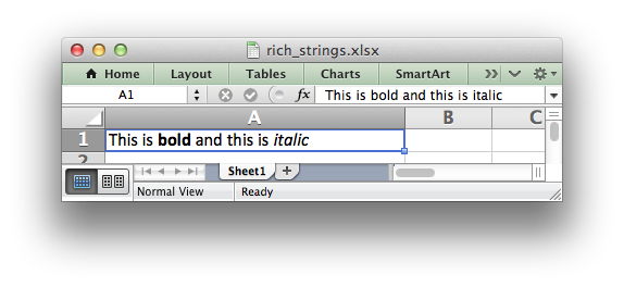
The write_rich_string() method is used to write strings with multiple
formats. For example to write the string “This is bold and this is
italic” you would use the following:
bold   = workbook.add_format({'bold': True})
italic = workbook.add_format({'italic': True})

worksheet.write_rich_string('A1',
                            'This is ',
                            bold, 'bold',
                            ' and this is ',
                            italic, 'italic')
Both row-column and A1 style notation are supported. The following are
equivalent:
worksheet.write_rich_string(0, 0, 'This is ', bold, 'bold')
worksheet.write_rich_string('A1', 'This is ', bold, 'bold')
See Working with Cell Notation for more details.
The basic rule is to break the string into fragments and put a
Format object before the fragment that you want to format.
For example:
# Unformatted string.
'This is an example string'

# Break it into fragments.
'This is an ', 'example', ' string'

# Add formatting before the fragments you want formatted.
'This is an ', format, 'example', ' string'

# In XlsxWriter.
worksheet.write_rich_string('A1',
                            'This is an ', format, 'example', ' string')
String fragments that don’t have a format are given a default format. So for
example when writing the string “Some bold text” you would use the first
example below but it would be equivalent to the second:
# Some bold format and a default format.
bold    = workbook.add_format({'bold': True})
default = workbook.add_format()

# With default formatting:
worksheet.write_rich_string('A1',
                            'Some ',
                            bold, 'bold',
                            ' text')

# Or more explicitly:
worksheet.write_rich_string('A1',
                             default, 'Some ',
                             bold,    'bold',
                             default, ' text')
If you have formats and segments in a list you can add them like this, using
the standard Python list unpacking syntax:
segments = ['This is ', bold, 'bold', ' and this is ', blue, 'blue']
worksheet.write_rich_string('A9', *segments)
In Excel only the font properties of the format such as font name, style, size,
underline, color and effects are applied to the string fragments in a rich
string. Other features such as border, background, text wrap and alignment
must be applied to the cell.
The write_rich_string() method allows you to do this by using the last
argument as a cell format (if it is a format object). The following example
centers a rich string in the cell:
bold   = workbook.add_format({'bold': True})
center = workbook.add_format({'align': 'center'})

worksheet.write_rich_string('A5',
                            'Some ',
                            bold, 'bold text',
                            ' centered',
                            center)
Note
Excel doesn’t allow the use of two consecutive formats in a rich string or
an empty string fragment. For either of these conditions a warning is
raised and the input to write_rich_string() is ignored.
Also, the maximum string size supported by Excel is 32,767 characters. If
the rich string exceeds this limit a warning is raised and the input to
write_rich_string() is ignored.
See also Example: Writing “Rich” strings with multiple formats and Example: Merging Cells with a Rich String.
worksheet.write_row()
-
write_row(row, col, data[, cell_format]) -
Write a row of data starting from (row, col).
Parameters: - row (int) – The cell row (zero indexed).
- col (int) – The cell column (zero indexed).
- data – Cell data to write. Variable types.
- cell_format (Format) – Optional Format object.
Returns: 0: Success.
Returns: Other: Error return value of the
write()method.
The write_row() method can be used to write a list of data in one go. This
is useful for converting the results of a database query into an Excel
worksheet. The write() method is called for each element of the data.
For example:
# Some sample data.
data = ('Foo', 'Bar', 'Baz')

# Write the data to a sequence of cells.
worksheet.write_row('A1', data)

# The above example is equivalent to:
worksheet.write('A1', data[0])
worksheet.write('B1', data[1])
worksheet.write('C1', data[2])
Both row-column and A1 style notation are supported. The following are
equivalent:
worksheet.write_row(0, 0, data)
worksheet.write_row('A1', data)
See Working with Cell Notation for more details.
worksheet.write_column()
-
write_column(row, col, data[, cell_format]) -
Write a column of data starting from (row, col).
Parameters: - row (int) – The cell row (zero indexed).
- col (int) – The cell column (zero indexed).
- data – Cell data to write. Variable types.
- cell_format (Format) – Optional Format object.
Returns: 0: Success.
Returns: Other: Error return value of the
write()method.
The write_column() method can be used to write a list of data in one go.
This is useful for converting the results of a database query into an Excel
worksheet. The write() method is called for each element of the data.
For example:
# Some sample data.
data = ('Foo', 'Bar', 'Baz')

# Write the data to a sequence of cells.
worksheet.write_column('A1', data)

# The above example is equivalent to:
worksheet.write('A1', data[0])
worksheet.write('A2', data[1])
worksheet.write('A3', data[2])
Both row-column and A1 style notation are supported. The following are
equivalent:
worksheet.write_column(0, 0, data)
worksheet.write_column('A1', data)
See Working with Cell Notation for more details.
worksheet.set_row()
-
set_row(row, height, cell_format, options) -
Set properties for a row of cells.
Parameters: - row (int) – The worksheet row (zero indexed).
- height (float) – The row height, in character units.
- cell_format (Format) – Optional Format object.
- options (dict) – Optional row parameters: hidden, level, collapsed.
Returns: 0: Success.
Returns: -1: Row is out of worksheet bounds.
The set_row() method is used to change the default properties of a row. The
most common use for this method is to change the height of a row:
worksheet.set_row(0, 20) # Set the height of Row 1 to 20.
The height is specified in character units. To specify the height in pixels
use the set_row_pixels() method.
The other common use for set_row() is to set the Format for
all cells in the row:
cell_format = workbook.add_format({'bold': True})

worksheet.set_row(0, 20, cell_format)
If you wish to set the format of a row without changing the default row height
you can pass None as the height parameter or use the default row height of
15:
worksheet.set_row(1, None, cell_format)
worksheet.set_row(1, 15,   cell_format)  # Same as above.
The cell_format parameter will be applied to any cells in the row that
don’t have a format. As with Excel it is overridden by an explicit cell
format. For example:
worksheet.set_row(0, None, format1)      # Row 1 has format1.

worksheet.write('A1', 'Hello')           # Cell A1 defaults to format1.
worksheet.write('B1', 'Hello', format2)  # Cell B1 keeps format2.
The options parameter is a dictionary with the following possible keys:
'hidden''level''collapsed'
Options can be set as follows:
worksheet.set_row(0, 20, cell_format, {'hidden': True})

# Or use defaults for other properties and set the options only.
worksheet.set_row(0, None, None, {'hidden': True})
The 'hidden' option is used to hide a row. This can be used, for example,
to hide intermediary steps in a complicated calculation:
worksheet.set_row(0, 20, cell_format, {'hidden': True})
The 'level' parameter is used to set the outline level of the row. Outlines
are described in Working with Outlines and Grouping. Adjacent rows with the same outline level
are grouped together into a single outline.
The following example sets an outline level of 1 for some rows:
worksheet.set_row(0, None, None, {'level': 1})
worksheet.set_row(1, None, None, {'level': 1})
worksheet.set_row(2, None, None, {'level': 1})
Excel allows up to 7 outline levels. The 'level' parameter should be in the
range 0 <= level <= 7.
The 'hidden' parameter can also be used to hide collapsed outlined rows
when used in conjunction with the 'level' parameter:
worksheet.set_row(1, None, None, {'hidden': 1, 'level': 1})
worksheet.set_row(2, None, None, {'hidden': 1, 'level': 1})
The 'collapsed' parameter is used in collapsed outlines to indicate which
row has the collapsed '+' symbol:
worksheet.set_row(3, None, None, {'collapsed': 1})
worksheet.set_row_pixels()
-
set_row_pixels(row, height, cell_format, options) -
Set properties for a row of cells, with the row height in pixels.
Parameters: - row (int) – The worksheet row (zero indexed).
- height (float) – The row height, in pixels.
- cell_format (Format) – Optional Format object.
- options (dict) – Optional row parameters: hidden, level, collapsed.
Returns: 0: Success.
Returns: -1: Row is out of worksheet bounds.
The set_row_pixels() method is identical to set_row() except that
the height can be set in pixels instead of Excel character units:
worksheet.set_row_pixels(0, 18) # Same as 24 in character units.
All other parameters and options are the same as set_row(). See the
documentation on set_row() for more details.
worksheet.set_column()
-
set_column(first_col, last_col, width, cell_format, options) -
Set properties for one or more columns of cells.
Parameters: - first_col (int) – First column (zero-indexed).
- last_col (int) – Last column (zero-indexed). Can be same as first_col.
- width (float) – The width of the column(s), in character units.
- cell_format (Format) – Optional Format object.
- options (dict) – Optional parameters: hidden, level, collapsed.
Returns: 0: Success.
Returns: -1: Column is out of worksheet bounds.
The set_column() method can be used to change the default properties of a
single column or a range of columns:
worksheet.set_column(1, 3, 30) # Width of columns B:D set to 30.
If set_column() is applied to a single column the value of first_col
and last_col should be the same:
worksheet.set_column(1, 1, 30) # Width of column B set to 30.
It is also possible, and generally clearer, to specify a column range using the
form of A1 notation used for columns. See Working with Cell Notation for more
details.
Examples:
worksheet.set_column(0, 0, 20)   # Column  A   width set to 20.
worksheet.set_column(1, 3, 30)   # Columns B-D width set to 30.
worksheet.set_column('E:E', 20)  # Column  E   width set to 20.
worksheet.set_column('F:H', 30)  # Columns F-H width set to 30.
The width parameter sets the column width in the same units used by Excel
which is: the number of characters in the default font. The default width is
8.43 in the default font of Calibri 11. The actual relationship between a
string width and a column width in Excel is complex. See the following
explanation of column widths
from the Microsoft support documentation for more details. To set the width in
pixels use the set_column_pixels() method.
See also the autofit() method for simulated autofitting of column widths.
As usual the cell_format Format parameter is optional. If
you wish to set the format without changing the default column width you can
pass None as the width parameter:
cell_format = workbook.add_format({'bold': True})

worksheet.set_column(0, 0, None, cell_format)
The cell_format parameter will be applied to any cells in the column that
don’t have a format. For example:
worksheet.set_column('A:A', None, format1)  # Col 1 has format1.

worksheet.write('A1', 'Hello')              # Cell A1 defaults to format1.
worksheet.write('A2', 'Hello', format2)     # Cell A2 keeps format2.
A row format takes precedence over a default column format:
worksheet.set_row(0, None, format1)         # Set format for row 1.
worksheet.set_column('A:A', None, format2)  # Set format for col 1.

worksheet.write('A1', 'Hello')              # Defaults to format1
worksheet.write('A2', 'Hello')              # Defaults to format2
The options parameter is a dictionary with the following possible keys:
'hidden''level''collapsed'
Options can be set as follows:
worksheet.set_column('D:D', 20, cell_format, {'hidden': 1})

# Or use defaults for other properties and set the options only.
worksheet.set_column('E:E', None, None, {'hidden': 1})
The 'hidden' option is used to hide a column. This can be used, for
example, to hide intermediary steps in a complicated calculation:
worksheet.set_column('D:D', 20, cell_format, {'hidden': 1})
The 'level' parameter is used to set the outline level of the column.
Outlines are described in Working with Outlines and Grouping. Adjacent columns with the same
outline level are grouped together into a single outline.
The following example sets an outline level of 1 for columns B to G:
worksheet.set_column('B:G', None, None, {'level': 1})
Excel allows up to 7 outline levels. The 'level' parameter should be in the
range 0 <= level <= 7.
The 'hidden' parameter can also be used to hide collapsed outlined columns
when used in conjunction with the 'level' parameter:
worksheet.set_column('B:G', None, None, {'hidden': 1, 'level': 1})
The 'collapsed' parameter is used in collapsed outlines to indicate which
column has the collapsed '+' symbol:
worksheet.set_column('H:H', None, None, {'collapsed': 1})
worksheet.set_column_pixels()
-
set_column_pixels(first_col, last_col, width, cell_format, options) -
Set properties for one or more columns of cells, with the width in pixels.
Parameters: - first_col (int) – First column (zero-indexed).
- last_col (int) – Last column (zero-indexed). Can be same as first_col.
- width (float) – The width of the column(s), in pixels.
- cell_format (Format) – Optional Format object.
- options (dict) – Optional parameters: hidden, level, collapsed.
Returns: 0: Success.
Returns: -1: Column is out of worksheet bounds.
The set_column_pixels() method is identical to set_column() except
that the width can be set in pixels instead of Excel character units:
worksheet.set_column_pixels(5, 5, 75) # Same as 10 character units.
![]()
All other parameters and options are the same as set_column(). See the
documentation on set_column() for more details.
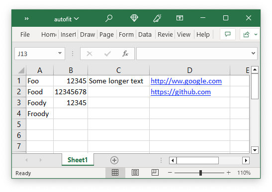
worksheet.autofit()
-
autofit() -
Simulates autofit for column widths.
Returns: Nothing.
The autofit() method can be used to simulate autofitting column widths based
on the largest string/number in the column:
See Example: Autofitting columns
There is no option in the xlsx file format that can be used to say “autofit
columns on loading”. Auto-fitting of columns is something that Excel does at
runtime when it has access to all of the worksheet information as well as the
Windows functions for calculating display areas based on fonts and formatting.
The worksheet.autofit() method simulates this behavior by calculating string
widths using metrics taken from Excel. As such there are some limitations to be
aware of when using this method:
- It is a simulated method and may not be accurate in all cases.
- It is based on the default font and font size of Calibri 11. It will not give
accurate results for other fonts or font sizes.
This isn’t perfect but for most cases it should be sufficient and if not you can
set your own widths, see below.
The autofit() method won’t override a user defined column width set with
set_column() or set_column_pixels() if it is greater than the autofit
value. This allows the user to set a minimum width value for a column.
You can also call set_column() and set_column_pixels() after
autofit() to override any of the calculated values.
worksheet.insert_image()
-
insert_image(row, col, filename[, options]) -
Insert an image in a worksheet cell.
Parameters: - row (int) – The cell row (zero indexed).
- col (int) – The cell column (zero indexed).
- filename – Image filename (with path if required).
- options (dict) – Optional parameters for image position, scale and url.
Returns: 0: Success.
Returns: -1: Row or column is out of worksheet bounds.
This method can be used to insert a image into a worksheet. The image can be in
PNG, JPEG, GIF, BMP, WMF or EMF format (see the notes about BMP and EMF below):
worksheet.insert_image('B2', 'python.png')
Both row-column and A1 style notation are supported. The following are
equivalent:
worksheet.insert_image(1, 1, 'python.png')
worksheet.insert_image('B2', 'python.png')
See Working with Cell Notation for more details.
A file path can be specified with the image name:
worksheet1.insert_image('B10', '../images/python.png')
worksheet2.insert_image('B20', r'c:imagespython.png')
The insert_image() method takes optional parameters in a dictionary to
position and scale the image. The available parameters with their default
values are:
{
    'x_offset':        0,
    'y_offset':        0,
    'x_scale':         1,
    'y_scale':         1,
    'object_position': 2,
    'image_data':      None,
    'url':             None,
    'description':     None,
    'decorative':      False,
}
The offset values are in pixels:
worksheet1.insert_image('B2', 'python.png', {'x_offset': 15, 'y_offset': 10})
The offsets can be greater than the width or height of the underlying cell.
This can be occasionally useful if you wish to align two or more images
relative to the same cell.
The x_scale and y_scale parameters can be used to scale the image
horizontally and vertically:
worksheet.insert_image('B3', 'python.png', {'x_scale': 0.5, 'y_scale': 0.5})
The url parameter can used to add a hyperlink/url to the image. The tip
parameter gives an optional mouseover tooltip for images with hyperlinks:
worksheet.insert_image('B4', 'python.png', {'url': 'https://python.org'})
See also write_url() for details on supported URIs.
The image_data parameter is used to add an in-memory byte stream in
io.BytesIO format:
worksheet.insert_image('B5', 'python.png', {'image_data': image_data})
This is generally used for inserting images from URLs:
url = 'https://python.org/logo.png'
image_data = io.BytesIO(urllib2.urlopen(url).read())

worksheet.insert_image('B5', url, {'image_data': image_data})
When using the image_data parameter a filename must still be passed to
insert_image() since it is used by Excel as a default description field
(see below). However, it can be a blank string if the description isn’t
required. In the previous example the filename/description is extracted from
the URL string. See also Example: Inserting images from a URL or byte stream into a worksheet.
The description field can be used to specify a description or “alt text”
string for the image. In general this would be used to provide a text
description of the image to help accessibility. It is an optional parameter
and defaults to the filename of the image. It can be used as follows:
worksheet.insert_image('B3', 'python.png',
                       {'description': 'The logo of the Python programming language.'})

The optional decorative parameter is also used to help accessibility. It
is used to mark the image as decorative, and thus uninformative, for automated
screen readers. As in Excel, if this parameter is in use the description
field isn’t written. It is used as follows:
worksheet.insert_image('B3', 'python.png', {'decorative': True})
The object_position parameter can be used to control the object
positioning of the image:
worksheet.insert_image('B3', 'python.png', {'object_position': 1})
Where object_position has the following allowable values:
- Move and size with cells.
- Move but don’t size with cells (the default).
- Don’t move or size with cells.
- Same as Option 1 to “move and size with cells” except XlsxWriter applies
hidden cells after the image is inserted.
See Working with Object Positioning for more detailed information about the positioning
and scaling of images within a worksheet.
Note
- BMP images are only supported for backward compatibility. In general it
is best to avoid BMP images since they aren’t compressed. If used, BMP
images must be 24 bit, true color, bitmaps. - EMF images can have very small differences in width and height when
compared to Excel files. Despite a lot of effort and testing it wasn’t
possible to exactly match Excel’s calculations for handling the
dimensions of EMF files. However, the differences are small (< 1%) and in
general aren’t visible.
See also Example: Inserting images into a worksheet.
worksheet.insert_chart()
-
insert_chart(row, col, chart[, options]) -
Write a string to a worksheet cell.
Parameters: - row (int) – The cell row (zero indexed).
- col (int) – The cell column (zero indexed).
- chart – A chart object.
- options (dict) – Optional parameters to position and scale the chart.
Returns: 0: Success.
Returns: -1: Row or column is out of worksheet bounds.
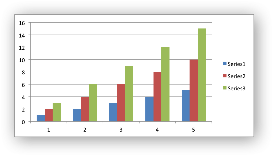
This method can be used to insert a chart into a worksheet. A chart object is
created via the Workbook add_chart() method where the chart type is
specified:
chart = workbook.add_chart({type, 'column'})
It is then inserted into a worksheet as an embedded chart:
worksheet.insert_chart('B5', chart)
Note
A chart can only be inserted into a worksheet once. If several similar
charts are required then each one must be created separately with
add_chart().
See The Chart Class, Working with Charts and Chart Examples.
Both row-column and A1 style notation are supported. The following are
equivalent:
worksheet.insert_chart(4, 1, chart)
worksheet.insert_chart('B5', chart)
See Working with Cell Notation for more details.
The insert_chart() method takes optional parameters in a dictionary to
position and scale the chart. The available parameters with their default
values are:
{
    'x_offset':        0,
    'y_offset':        0,
    'x_scale':         1,
    'y_scale':         1,
    'object_position': 1,
    'description':     None,
    'decorative':      False,
}
The offset values are in pixels:
worksheet.insert_chart('B5', chart, {'x_offset': 25, 'y_offset': 10})
The x_scale and y_scale parameters can be used to scale the chart
horizontally and vertically:
worksheet.insert_chart('B5', chart, {'x_scale': 0.5, 'y_scale': 0.5})
These properties can also be set via the Chart set_size() method.
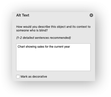
The description field can be used to specify a description or “alt text”
string for the chart. In general this would be used to provide a text
description of the chart to help accessibility. It is an optional parameter
and has no default. It can be used as follows:
worksheet.insert_chart('B5', chart,
                       {'description': 'Chart showing sales for the current year'})
The optional decorative parameter is also used to help accessibility. It
is used to mark the chart as decorative, and thus uninformative, for automated
screen readers. As in Excel, if this parameter is in use the description
field isn’t written. It is used as follows:
worksheet.insert_chart('B5', chart, {'decorative': True})
The object_position parameter can be used to control the object
positioning of the chart:
worksheet.insert_chart('B5', chart, {'object_position': 2})
Where object_position has the following allowable values:
- Move and size with cells (the default).
- Move but don’t size with cells.
- Don’t move or size with cells.
See Working with Object Positioning for more detailed information about the positioning
and scaling of charts within a worksheet.
worksheet.insert_textbox()
-
insert_textbox(row, col, textbox[, options]) -
Write a string to a worksheet cell.
Parameters: - row (int) – The cell row (zero indexed).
- col (int) – The cell column (zero indexed).
- text (string) – The text in the textbox.
- options (dict) – Optional parameters to position and scale the textbox.
Returns: 0: Success.
Returns: -1: Row or column is out of worksheet bounds.
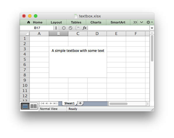
This method can be used to insert a textbox into a worksheet:
worksheet.insert_textbox('B2', 'A simple textbox with some text')
Both row-column and A1 style notation are supported. The following are
equivalent:
worksheet.insert_textbox(1, 1, 'Some text')
worksheet.insert_textbox('B2', 'Some text')
See Working with Cell Notation for more details.
The size and formatting of the textbox can be controlled via the options dict:
# Size and position
width
height
x_scale
y_scale
x_offset
y_offset
object_position

# Formatting
line
border
fill
gradient
font
align
text_rotation

# Links
textlink
url
tip

# Accessibility
description
decorative
These options are explained in more detail in the
Working with Textboxes section.
See also Example: Insert Textboxes into a Worksheet.
See Working with Object Positioning for more detailed information about the positioning
and scaling of images within a worksheet.
worksheet.insert_button()
-
insert_button(row, col[, options]) -
Insert a VBA button control on a worksheet.
Parameters: - row (int) – The cell row (zero indexed).
- col (int) – The cell column (zero indexed).
- options (dict) – Optional parameters to position and scale the button.
Returns: 0: Success.
Returns: -1: Row or column is out of worksheet bounds.
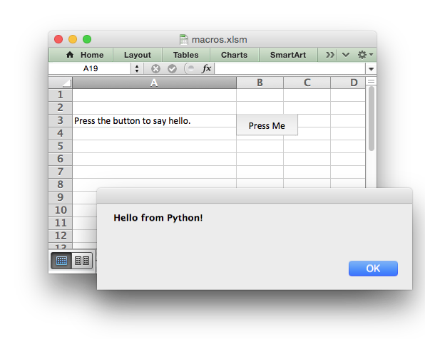
The insert_button() method can be used to insert an Excel form button into a worksheet.
This method is generally only useful when used in conjunction with the
Workbook add_vba_project() method to tie the button to a macro from an
embedded VBA project:
# Add the VBA project binary.
workbook.add_vba_project('./vbaProject.bin')

# Add a button tied to a macro in the VBA project.
worksheet.insert_button('B3', {'macro':   'say_hello',
                               'caption': 'Press Me'})
See Working with VBA Macros and Example: Adding a VBA macro to a Workbook for more details.
Both row-column and A1 style notation are supported. The following are
equivalent:
worksheet.insert_button(2, 1, {'macro':   'say_hello',
                               'caption': 'Press Me'})

worksheet.insert_button('B3', {'macro':   'say_hello',
                               'caption': 'Press Me'})
See Working with Cell Notation for more details.
The insert_button() method takes optional parameters in a dictionary to
position and scale the chart. The available parameters with their default
values are:
{
    'macro':       None,
    'caption':     'Button 1',
    'width':       64,
    'height':      20.
    'x_offset':    0,
    'y_offset':    0,
    'x_scale':     1,
    'y_scale':     1,
    'description': None,
}
The macro option is used to set the macro that the button will invoke when
the user clicks on it. The macro should be included using the Workbook
add_vba_project() method shown above.
The caption is used to set the caption on the button. The default is
Button n where n is the button number.
The default button width is 64 pixels which is the width of a default cell
and the default button height is 20 pixels which is the height of a
default cell.
The offset, scale and description options are the same as for
insert_chart(), see above.
worksheet.data_validation()
-
data_validation(first_row, first_col, last_row, last_col, options) -
Write a conditional format to range of cells.
Parameters: - first_row (int) – The first row of the range. (All zero indexed.)
- first_col (int) – The first column of the range.
- last_row (int) – The last row of the range.
- last_col (int) – The last col of the range.
- options (dict) – Data validation options.
Returns: 0: Success.
Returns: -1: Row or column is out of worksheet bounds.
Returns: -2: Incorrect parameter or option.
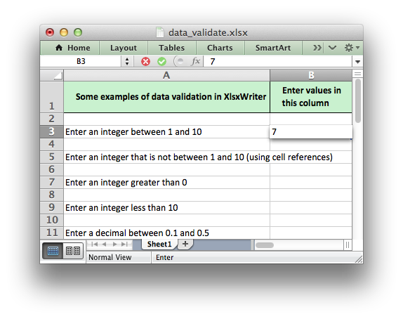
The data_validation() method is used to construct an Excel data validation
or to limit the user input to a dropdown list of values:
worksheet.data_validation('B3', {'validate': 'integer',
                                 'criteria': 'between',
                                 'minimum': 1,
                                 'maximum': 10})


worksheet.data_validation('B13', {'validate': 'list',
                                  'source': ['open', 'high', 'close']})
The data validation can be applied to a single cell or a range of cells. As
usual you can use A1 or Row/Column notation, see Working with Cell Notation:
worksheet.data_validation(1, 1, {'validate': 'list',
                                 'source': ['open', 'high', 'close']})

worksheet.data_validation('B2', {'validate': 'list',
                                 'source': ['open', 'high', 'close']})
With Row/Column notation you must specify all four cells in the range:
(first_row, first_col, last_row, last_col). If you need to refer to a
single cell set the last_ values equal to the first_ values. With A1
notation you can refer to a single cell or a range of cells:
worksheet.data_validation(0, 0, 4, 1, {...})
worksheet.data_validation('B1',       {...})
worksheet.data_validation('C1:E5',    {...})
The options parameter in data_validation() must be a dictionary containing
the parameters that describe the type and style of the data validation. There
are a lot of available options which are described in detail in a separate
section: Working with Data Validation. See also Example: Data Validation and Drop Down Lists.
worksheet.conditional_format()
-
conditional_format(first_row, first_col, last_row, last_col, options) -
Write a conditional format to range of cells.
Parameters: - first_row (int) – The first row of the range. (All zero indexed.)
- first_col (int) – The first column of the range.
- last_row (int) – The last row of the range.
- last_col (int) – The last col of the range.
- options (dict) – Conditional formatting options.
Returns: 0: Success.
Returns: -1: Row or column is out of worksheet bounds.
Returns: -2: Incorrect parameter or option.
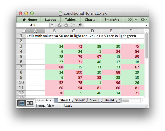
The conditional_format() method is used to add formatting to a cell or
range of cells based on user defined criteria:
worksheet.conditional_format('B3:K12', {'type':     'cell',
                                        'criteria': '>=',
                                        'value':    50,
                                        'format':   format1})
The conditional format can be applied to a single cell or a range of cells. As
usual you can use A1 or Row/Column notation, see Working with Cell Notation:
worksheet.conditional_format(0, 0, 2, 1, {'type':     'cell',
                                          'criteria': '>=',
                                          'value':    50,
                                          'format':   format1})

# This is equivalent to the following:
worksheet.conditional_format('A1:B3', {'type':     'cell',
                                        'criteria': '>=',
                                        'value':    50,
                                        'format':   format1})
With Row/Column notation you must specify all four cells in the range:
(first_row, first_col, last_row, last_col). If you need to refer to a
single cell set the last_ values equal to the first_ values. With A1
notation you can refer to a single cell or a range of cells:
worksheet.conditional_format(0, 0, 4, 1, {...})
worksheet.conditional_format('B1',       {...})
worksheet.conditional_format('C1:E5',    {...})
The options parameter in conditional_format() must be a dictionary
containing the parameters that describe the type and style of the conditional
format. There are a lot of available options which are described in detail in
a separate section: Working with Conditional Formatting. See also
Example: Conditional Formatting.
worksheet.add_table()
-
add_table(first_row, first_col, last_row, last_col, options) -
Add an Excel table to a worksheet.
Parameters: - first_row (int) – The first row of the range. (All zero indexed.)
- first_col (int) – The first column of the range.
- last_row (int) – The last row of the range.
- last_col (int) – The last col of the range.
- options (dict) – Table formatting options. (Optional)
Raises: OverlappingRange – if the range overlaps a previous merge or table range.
Returns: 0: Success.
Returns: -1: Row or column is out of worksheet bounds.
Returns: -2: Incorrect parameter or option.
Returns: -3: Not supported in
constant_memorymode.
The add_table() method is used to group a range of cells into an Excel
Table:
worksheet.add_table('B3:F7', { ... })
This method contains a lot of parameters and is described in Working with Worksheet Tables.
Both row-column and A1 style notation are supported. The following are
equivalent:
worksheet.add_table(2, 1, 6, 5, { ... })
worksheet.add_table('B3:F7',    { ... })
See Working with Cell Notation for more details.
See also the examples in Example: Worksheet Tables.
Note
Tables aren’t available in XlsxWriter when Workbook()
'constant_memory' mode is enabled.
worksheet.add_sparkline()
-
add_sparkline(row, col, options) -
Add sparklines to a worksheet.
Parameters: - row (int) – The cell row (zero indexed).
- col (int) – The cell column (zero indexed).
- options (dict) – Sparkline formatting options.
Returns: 0: Success.
Returns: -1: Row or column is out of worksheet bounds.
Returns: -2: Incorrect parameter or option.
Sparklines are small charts that fit in a single cell and are used to show
trends in data.
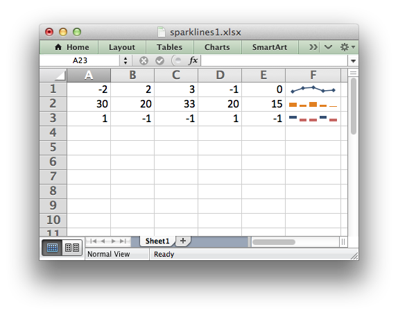
The add_sparkline() worksheet method is used to add sparklines to a cell or
a range of cells:
worksheet.add_sparkline('F1', {'range': 'A1:E1'})
Both row-column and A1 style notation are supported. The following are
equivalent:
worksheet.add_sparkline(0, 5, {'range': 'A1:E1'})
worksheet.add_sparkline('F1', {'range': 'A1:E1'})
See Working with Cell Notation for more details.
This method contains a lot of parameters and is described in detail in
Working with Sparklines.
See also Example: Sparklines (Simple) and Example: Sparklines (Advanced).
Note
Sparklines are a feature of Excel 2010+ only. You can write them to
an XLSX file that can be read by Excel 2007 but they won’t be displayed.
worksheet.get_name()
-
get_name() -
Retrieve the worksheet name.
The get_name() method is used to retrieve the name of a worksheet. This is
something useful for debugging or logging:
for worksheet in workbook.worksheets():
    print worksheet.get_name()
There is no set_name() method. The only safe way to set the worksheet name
is via the add_worksheet() method.
worksheet.activate()
-
activate() -
Make a worksheet the active, i.e., visible worksheet.
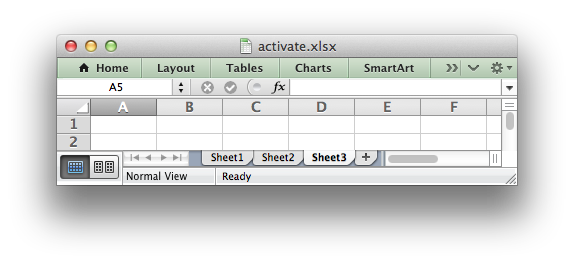
The activate() method is used to specify which worksheet is initially
visible in a multi-sheet workbook:
worksheet1 = workbook.add_worksheet()
worksheet2 = workbook.add_worksheet()
worksheet3 = workbook.add_worksheet()

worksheet3.activate()
More than one worksheet can be selected via the select() method, see below,
however only one worksheet can be active.
The default active worksheet is the first worksheet.
worksheet.select()
-
select() -
Set a worksheet tab as selected.
The select() method is used to indicate that a worksheet is selected in a
multi-sheet workbook:
worksheet1.activate()
worksheet2.select()
worksheet3.select()
A selected worksheet has its tab highlighted. Selecting worksheets is a way of
grouping them together so that, for example, several worksheets could be
printed in one go. A worksheet that has been activated via the activate()
method will also appear as selected.
worksheet.hide()
-
hide() -
Hide the current worksheet.
The hide() method is used to hide a worksheet:
You may wish to hide a worksheet in order to avoid confusing a user with
intermediate data or calculations.
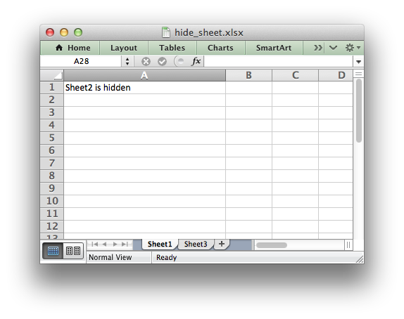
A hidden worksheet can not be activated or selected so this method is mutually
exclusive with the activate() and select() methods. In
addition, since the first worksheet will default to being the active
worksheet, you cannot hide the first worksheet without activating another
sheet:
worksheet2.activate()
worksheet1.hide()
See Example: Hiding Worksheets for more details.
worksheet.set_first_sheet()
-
set_first_sheet() -
Set current worksheet as the first visible sheet tab.
The activate() method determines which worksheet is initially selected.
However, if there are a large number of worksheets the selected worksheet may
not appear on the screen. To avoid this you can select which is the leftmost
visible worksheet tab using set_first_sheet():
for in range(1, 21):
    workbook.add_worksheet

worksheet19.set_first_sheet()  # First visible worksheet tab.
worksheet20.activate()         # First visible worksheet.
This method is not required very often. The default value is the first
worksheet.
worksheet.merge_range()
-
merge_range(first_row, first_col, last_row, last_col, data[, cell_format]) -
Merge a range of cells.
Parameters: - first_row (int) – The first row of the range. (All zero indexed.)
- first_col (int) – The first column of the range.
- last_row (int) – The last row of the range.
- last_col (int) – The last col of the range.
- data – Cell data to write. Variable types.
- cell_format (Format) – Optional Format object.
Raises: OverlappingRange – if the range overlaps a previous merge or table range.
Returns: 0: Success.
Returns: -1: Row or column is out of worksheet bounds.
Returns: Other: Error return value of the called
write()method.
The merge_range() method allows cells to be merged together so that they
act as a single area.
Excel generally merges and centers cells at same time. To get similar behavior
with XlsxWriter you need to apply a Format:
merge_format = workbook.add_format({'align': 'center'})

worksheet.merge_range('B3:D4', 'Merged Cells', merge_format)
Both row-column and A1 style notation are supported. The following are
equivalent:
worksheet.merge_range(2, 1, 3, 3, 'Merged Cells', merge_format)
worksheet.merge_range('B3:D4',    'Merged Cells', merge_format)
See Working with Cell Notation for more details.
It is possible to apply other formatting to the merged cells as well:
merge_format = workbook.add_format({
    'bold':     True,
    'border':   6,
    'align':    'center',
    'valign':   'vcenter',
    'fg_color': '#D7E4BC',
})

worksheet.merge_range('B3:D4', 'Merged Cells', merge_format)
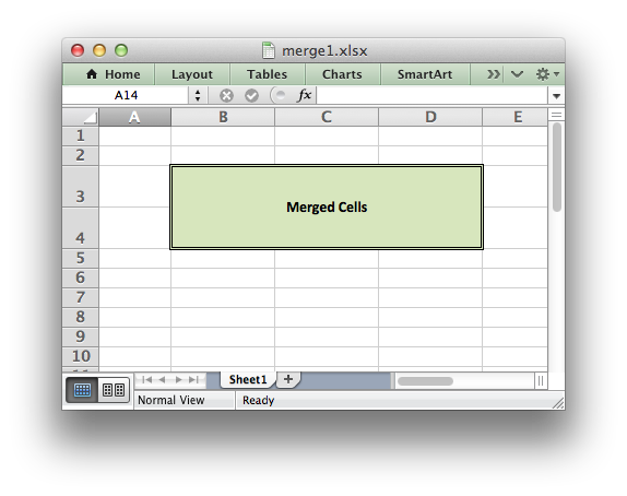
See Example: Merging Cells for more details.
The merge_range() method writes its data argument using
write(). Therefore it will handle numbers, strings and formulas as
usual. If this doesn’t handle your data correctly then you can overwrite the
first cell with a call to one of the other
write_*() methods using the same Format as in the merged cells. See Example: Merging Cells with a Rich String.
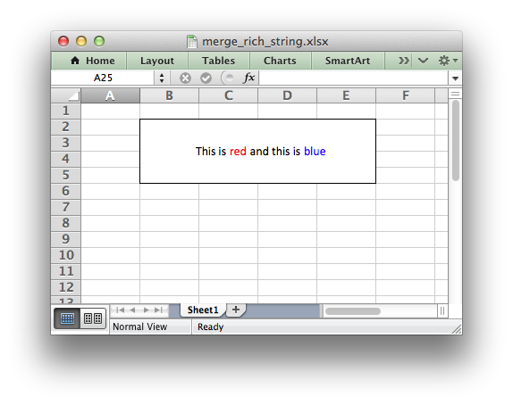
Note
Merged ranges generally don’t work in XlsxWriter when Workbook()
'constant_memory' mode is enabled.
worksheet.autofilter()
-
autofilter(first_row, first_col, last_row, last_col) -
Set the autofilter area in the worksheet.
Parameters: - first_row (int) – The first row of the range. (All zero indexed.)
- first_col (int) – The first column of the range.
- last_row (int) – The last row of the range.
- last_col (int) – The last col of the range.
The autofilter() method allows an autofilter to be added to a worksheet. An
autofilter is a way of adding drop down lists to the headers of a 2D range of
worksheet data. This allows users to filter the data based on simple criteria
so that some data is shown and some is hidden.
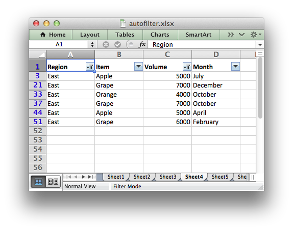
To add an autofilter to a worksheet:
worksheet.autofilter('A1:D11')
Both row-column and A1 style notation are supported. The following are
equivalent:
worksheet.autofilter(0, 0, 10, 3)
worksheet.autofilter('A1:D11')
See Working with Cell Notation for more details.
Filter conditions can be applied using the filter_column() or
filter_column_list() methods.
See Working with Autofilters for more details.
worksheet.filter_column()
-
filter_column(col, criteria) -
Set the column filter criteria.
Parameters: - col (int) – Filter column (zero-indexed).
- criteria (string) – Filter criteria.
The filter_column method can be used to filter columns in a autofilter
range based on simple conditions.
The conditions for the filter are specified using simple expressions:
worksheet.filter_column('A', 'x > 2000')
worksheet.filter_column('B', 'x > 2000 and x < 5000')
The col parameter can either be a zero indexed column number or a string
column name:
worksheet.filter_column(2,   'x > 2000')
worksheet.filter_column('C', 'x > 2000')
See Working with Cell Notation for more details.
It isn’t sufficient to just specify the filter condition. You must also hide
any rows that don’t match the filter condition. See
Working with Autofilters for more details.
worksheet.filter_column_list()
-
filter_column_list(col, filters) -
Set the column filter criteria in Excel 2007 list style.
Parameters: - col (int) – Filter column (zero-indexed).
- filters (list) – List of filter criteria to match.
The filter_column_list() method can be used to represent filters with
multiple selected criteria:
worksheet.filter_column_list('A', ['March', 'April', 'May'])
The col parameter can either be a zero indexed column number or a string
column name:
worksheet.filter_column_list(2,   ['March', 'April', 'May'])
worksheet.filter_column_list('C', ['March', 'April', 'May'])
See Working with Cell Notation for more details.
One or more criteria can be selected:
worksheet.filter_column_list('A', ['March'])
worksheet.filter_column_list('C', [100, 110, 120, 130])
To filter blanks as part of the list use Blanks as a list item:
worksheet.filter_column_list('A', ['March', 'April', 'May', 'Blanks'])
It isn’t sufficient to just specify filters. You must also hide any rows that
don’t match the filter condition. See Working with Autofilters for more
details.
worksheet.set_selection()
-
set_selection(first_row, first_col, last_row, last_col) -
Set the selected cell or cells in a worksheet.
Parameters: - first_row (int) – The first row of the range. (All zero indexed.)
- first_col (int) – The first column of the range.
- last_row (int) – The last row of the range.
- last_col (int) – The last col of the range.
The set_selection() method can be used to specify which cell or range of
cells is selected in a worksheet. The most common requirement is to select a
single cell, in which case the first_ and last_ parameters should be
the same.
The active cell within a selected range is determined by the order in which
first_ and last_ are specified.
Examples:
worksheet1.set_selection(3, 3, 3, 3)  # 1. Cell D4.
worksheet2.set_selection(3, 3, 6, 6)  # 2. Cells D4 to G7.
worksheet3.set_selection(6, 6, 3, 3)  # 3. Cells G7 to D4.
worksheet4.set_selection('D4')        # Same as 1.
worksheet5.set_selection('D4:G7')     # Same as 2.
worksheet6.set_selection('G7:D4')     # Same as 3.
As shown above, both row-column and A1 style notation are supported. See
Working with Cell Notation for more details. The default cell selection is
(0, 0), 'A1'.
worksheet.set_top_left_cell()
-
set_top_left_cell(row, col) -
Set the first visible cell at the top left of a worksheet.
Parameters: - row (int) – The cell row (zero indexed).
- col (int) – The cell column (zero indexed).
This set_top_left_cell method can be used to set the top leftmost visible
cell in the worksheet:
worksheet.set_top_left_cell(31, 26)

# Same as:
worksheet.set_top_left_cell('AA32')
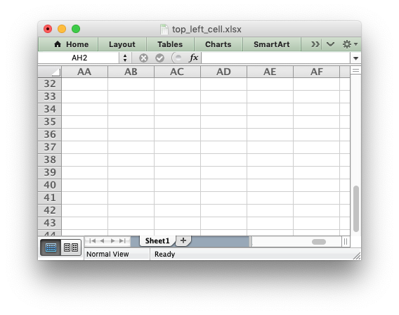
As shown above, both row-column and A1 style notation are supported. See
Working with Cell Notation for more details.
worksheet.freeze_panes()
-
freeze_panes(row, col[, top_row, left_col]) -
Create worksheet panes and mark them as frozen.
Parameters: - row (int) – The cell row (zero indexed).
- col (int) – The cell column (zero indexed).
- top_row (int) – Topmost visible row in scrolling region of pane.
- left_col (int) – Leftmost visible row in scrolling region of pane.
The freeze_panes() method can be used to divide a worksheet into horizontal
or vertical regions known as panes and to “freeze” these panes so that the
splitter bars are not visible.
The parameters row and col are used to specify the location of the
split. It should be noted that the split is specified at the top or left of a
cell and that the method uses zero based indexing. Therefore to freeze the
first row of a worksheet it is necessary to specify the split at row 2 (which
is 1 as the zero-based index).
You can set one of the row and col parameters as zero if you do not
want either a vertical or horizontal split.
Examples:
worksheet.freeze_panes(1, 0)  # Freeze the first row.
worksheet.freeze_panes('A2')  # Same using A1 notation.
worksheet.freeze_panes(0, 1)  # Freeze the first column.
worksheet.freeze_panes('B1')  # Same using A1 notation.
worksheet.freeze_panes(1, 2)  # Freeze first row and first 2 columns.
worksheet.freeze_panes('C2')  # Same using A1 notation.
As shown above, both row-column and A1 style notation are supported. See
Working with Cell Notation for more details.
The parameters top_row and left_col are optional. They are used to
specify the top-most or left-most visible row or column in the scrolling
region of the panes. For example to freeze the first row and to have the
scrolling region begin at row twenty:
worksheet.freeze_panes(1, 0, 20, 0)
You cannot use A1 notation for the top_row and left_col parameters.
See Example: Freeze Panes and Split Panes for more details.
worksheet.split_panes()
-
split_panes(x, y[, top_row, left_col]) -
Create worksheet panes and mark them as split.
Parameters: - x (float) – The position for the vertical split.
- y (float) – The position for the horizontal split.
- top_row (int) – Topmost visible row in scrolling region of pane.
- left_col (int) – Leftmost visible row in scrolling region of pane.
The split_panes method can be used to divide a worksheet into horizontal
or vertical regions known as panes. This method is different from the
freeze_panes() method in that the splits between the panes will be visible
to the user and each pane will have its own scroll bars.
The parameters y and x are used to specify the vertical and horizontal
position of the split. The units for y and x are the same as those
used by Excel to specify row height and column width. However, the vertical
and horizontal units are different from each other. Therefore you must specify
the y and x parameters in terms of the row heights and column widths
that you have set or the default values which are 15 for a row and
8.43 for a column.
You can set one of the y and x parameters as zero if you do not want
either a vertical or horizontal split. The parameters top_row and
left_col are optional. They are used to specify the top-most or left-most
visible row or column in the bottom-right pane.
Example:
worksheet.split_panes(15, 0)     # First row.
worksheet.split_panes(0, 8.43)   # First column.
worksheet.split_panes(15, 8.43)  # First row and column.
You cannot use A1 notation with this method.
See Example: Freeze Panes and Split Panes for more details.
worksheet.set_zoom()
-
set_zoom(zoom) -
Set the worksheet zoom factor.
Parameters: zoom (int) – Worksheet zoom factor.
Set the worksheet zoom factor in the range 10 <= zoom <= 400:
worksheet1.set_zoom(50)
worksheet2.set_zoom(75)
worksheet3.set_zoom(300)
worksheet4.set_zoom(400)
The default zoom factor is 100. It isn’t possible to set the zoom to
“Selection” because it is calculated by Excel at run-time.
Note, set_zoom() does not affect the scale of the printed page. For that
you should use set_print_scale().
worksheet.right_to_left()
-
right_to_left() -
Display the worksheet cells from right to left for some versions of Excel.
The right_to_left() method is used to change the default direction of the
worksheet from left-to-right, with the A1 cell in the top left, to
right-to-left, with the A1 cell in the top right:
worksheet.right_to_left()
This is useful when creating Arabic, Hebrew or other near or far eastern
worksheets that use right-to-left as the default direction.
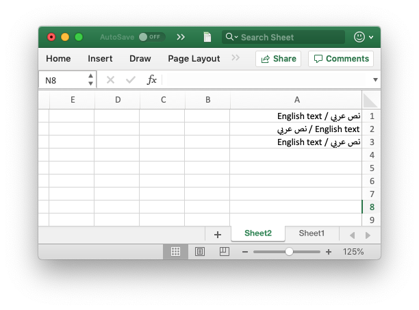
See also the Format set_reading_order() property to set the direction of the
text within cells and the Example: Left to Right worksheets and text example program.
worksheet.hide_zero()
-
hide_zero() -
Hide zero values in worksheet cells.
The hide_zero() method is used to hide any zero values that appear in
cells:
worksheet.set_background()
-
set_background(filename[, is_byte_stream]) -
Set the background image for a worksheet.
Parameters: - filename (str) – The image file (or byte stream).
- is_byte_stream (bool) – The file is a stream of bytes.
The set_background() method can be used to set the background image for the
worksheet:
worksheet.set_background('logo.png')
The set_background() method supports all the image formats supported by
insert_image().
Some people use this method to add a watermark background to their
document. However, Microsoft recommends using a header image to set a
watermark.
The choice of method depends on whether you want the watermark to be visible
in normal viewing mode or just when the file is printed. In XlsxWriter you can
get the header watermark effect using set_header():
worksheet.set_header('&C&G', {'image_center': 'watermark.png'})
It is also possible to pass an in-memory byte stream to set_background()
if the is_byte_stream parameter is set to True. The stream should be
io.BytesIO:
worksheet.set_background(io_bytes, is_byte_stream=True)
See Example: Setting the Worksheet Background for an example.
worksheet.set_tab_color()
-
set_tab_color() -
Set the color of the worksheet tab.
Parameters: color (string) – The tab color.
The set_tab_color() method is used to change the color of the worksheet
tab:
worksheet1.set_tab_color('red')
worksheet2.set_tab_color('#FF9900')  # Orange
The color can be a Html style #RRGGBB string or a limited number named
colors, see Working with Colors.
See Example: Setting Worksheet Tab Colors for more details.
worksheet.protect()
-
protect() -
Protect elements of a worksheet from modification.
Parameters: - password (string) – A worksheet password.
- options (dict) – A dictionary of worksheet options to protect.
The protect() method is used to protect a worksheet from modification:
The protect() method also has the effect of enabling a cell’s locked
and hidden properties if they have been set. A locked cell cannot be
edited and this property is on by default for all cells. A hidden cell will
display the results of a formula but not the formula itself. These properties
can be set using the set_locked() and set_hidden() format methods.
You can optionally add a password to the worksheet protection:
worksheet.protect('abc123')
The password should be an ASCII string. Passing the empty string '' is the
same as turning on protection without a password. See the note below on the
“password” strength.
You can specify which worksheet elements you wish to protect by passing a
dictionary in the options argument with any or all of the following keys:
# Default values shown.
options = {
    'objects':               False,
    'scenarios':             False,
    'format_cells':          False,
    'format_columns':        False,
    'format_rows':           False,
    'insert_columns':        False,
    'insert_rows':           False,
    'insert_hyperlinks':     False,
    'delete_columns':        False,
    'delete_rows':           False,
    'select_locked_cells':   True,
    'sort':                  False,
    'autofilter':            False,
    'pivot_tables':          False,
    'select_unlocked_cells': True,
}
The default boolean values are shown above. Individual elements can be
protected as follows:
worksheet.protect('abc123', {'insert_rows': True})
For chartsheets the allowable options and default values are:
options = {
    'objects':               True,
    'content':               True,
}
See also the set_locked() and set_hidden() format methods and
Example: Enabling Cell protection in Worksheets.
Note
Worksheet level passwords in Excel offer very weak protection. They do not
encrypt your data and are very easy to deactivate. Full workbook encryption
is not supported by XlsxWriter. However, it is possible to encrypt an
XlsxWriter file using a third party open source tool called msoffice-crypt. This works for macOS, Linux and
Windows:
msoffice-crypt.exe -e -p password clear.xlsx encrypted.xlsx
worksheet.unprotect_range()
-
unprotect_range(cell_range, range_name) -
Unprotect ranges within a protected worksheet.
Parameters: - cell_range (string) – The cell or cell range to unprotect.
- range_name (string) – An name for the range.
The unprotect_range() method is used to unprotect ranges in a protected
worksheet. It can be used to set a single range or multiple ranges:
worksheet.unprotect_range('A1')
worksheet.unprotect_range('C1')
worksheet.unprotect_range('E1:E3')
worksheet.unprotect_range('G1:K100')
As in Excel the ranges are given sequential names like Range1 and
Range2 but a user defined name can also be specified:
worksheet.unprotect_range('G4:I6', 'MyRange')
worksheet.set_default_row()
-
set_default_row(height, hide_unused_rows) -
Set the default row properties.
Parameters: - height (float) – Default height. Optional, defaults to 15.
- hide_unused_rows (bool) – Hide unused rows. Optional, defaults to False.
The set_default_row() method is used to set the limited number of default
row properties allowed by Excel which are the default height and the option to
hide unused rows. These parameters are an optimization used by Excel to set
row properties without generating a very large file with an entry for each row.
To set the default row height:
worksheet.set_default_row(24)
To hide unused rows:
worksheet.set_default_row(hide_unused_rows=True)
See Example: Hiding Rows and Columns for more details.
worksheet.outline_settings()
-
outline_settings(visible, symbols_below, symbols_right, auto_style) -
Control outline settings.
Parameters: - visible (bool) – Outlines are visible. Optional, defaults to True.
- symbols_below (bool) – Show row outline symbols below the outline bar.
Optional, defaults to True. - symbols_right (bool) – Show column outline symbols to the right of the
outline bar. Optional, defaults to True. - auto_style (bool) – Use Automatic style. Optional, defaults to False.
The outline_settings() method is used to control the appearance of outlines
in Excel. Outlines are described in Working with Outlines and Grouping:
worksheet1.outline_settings(False, False, False, True)
The 'visible' parameter is used to control whether or not outlines are
visible. Setting this parameter to False will cause all outlines on the
worksheet to be hidden. They can be un-hidden in Excel by means of the “Show
Outline Symbols” command button. The default setting is True for visible
outlines.
The 'symbols_below' parameter is used to control whether the row outline
symbol will appear above or below the outline level bar. The default setting
is True for symbols to appear below the outline level bar.
The 'symbols_right' parameter is used to control whether the column outline
symbol will appear to the left or the right of the outline level bar. The
default setting is True for symbols to appear to the right of the outline
level bar.
The 'auto_style' parameter is used to control whether the automatic outline
generator in Excel uses automatic styles when creating an outline. This has no
effect on a file generated by XlsxWriter but it does have an effect on how
the worksheet behaves after it is created. The default setting is False
for “Automatic Styles” to be turned off.
The default settings for all of these parameters correspond to Excel’s default
parameters.
The worksheet parameters controlled by outline_settings() are rarely used.
worksheet.set_vba_name()
-
set_vba_name(name) -
Set the VBA name for the worksheet.
Parameters: name (string) – The VBA name for the worksheet.
The set_vba_name() method can be used to set the VBA codename for the
worksheet (there is a similar method for the workbook VBA name). This is
sometimes required when a vbaProject macro included via add_vba_project()
refers to the worksheet. The default Excel VBA name of Sheet1, etc., is
used if a user defined name isn’t specified.
See Working with VBA Macros for more details.
worksheet.ignore_errors()
-
ignore_errors(options) -
Ignore various Excel errors/warnings in a worksheet for user defined
ranges.Returns: 0: Success. Returns: -1: Incorrect parameter or option.
The ignore_errors() method can be used to ignore various worksheet cell
errors/warnings. For example the following code writes a string that looks
like a number:
worksheet.write_string('D2', '123')
This causes Excel to display a small green triangle in the top left hand
corner of the cell to indicate an error/warning:
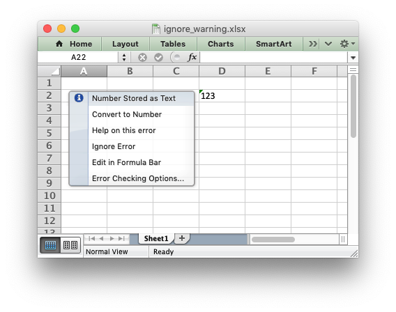
Sometimes these warnings are useful indicators that there is an issue in the
spreadsheet but sometimes it is preferable to turn them off. Warnings can be
turned off at the Excel level for all workbooks and worksheets by using the
using “Excel options -> Formulas -> Error checking rules”. Alternatively you
can turn them off for individual cells in a worksheet, or ranges of cells,
using the ignore_errors() method with a dict of options and ranges like
this:
worksheet.ignore_errors({'number_stored_as_text': 'A1:H50'})

# Or for more than one option:
worksheet.ignore_errors({'number_stored_as_text': 'A1:H50',
                         'eval_error':            'A1:H50'})
The range can be a single cell, a range of cells, or multiple cells and ranges
separated by spaces:
# Single cell.
worksheet.ignore_errors({'eval_error': 'C6'})

# Or a single range:
worksheet.ignore_errors({'eval_error': 'C6:G8'})

# Or multiple cells and ranges:
worksheet.ignore_errors({'eval_error': 'C6 E6 G1:G20 J2:J6'})
Note: calling ignore_errors() multiple times will overwrite the previous
settings.
You can turn off warnings for an entire column by specifying the range from
the first cell in the column to the last cell in the column:
worksheet.ignore_errors({'number_stored_as_text': 'A1:A1048576'})
Or for the entire worksheet by specifying the range from the first cell in the
worksheet to the last cell in the worksheet:
worksheet.ignore_errors({'number_stored_as_text': 'A1:XFD1048576'})
The worksheet errors/warnings that can be ignored are:
number_stored_as_text: Turn off errors/warnings for numbers stores as
text.eval_error: Turn off errors/warnings for formula errors (such as divide
by zero).formula_differs: Turn off errors/warnings for formulas that differ from
surrounding formulas.formula_range: Turn off errors/warnings for formulas that omit cells in
a range.formula_unlocked: Turn off errors/warnings for unlocked cells that
contain formulas.empty_cell_reference: Turn off errors/warnings for formulas that refer
to empty cells.list_data_validation: Turn off errors/warnings for cells in a table that
do not comply with applicable data validation rules.calculated_column: Turn off errors/warnings for cell formulas that
differ from the column formula.two_digit_text_year: Turn off errors/warnings for formulas that contain
a two digit text representation of a year.
See also Example: Ignoring Worksheet errors and warnings.
Tuesday, February 27, 2018
How merged Cells in Excel being handled by Pandas data frame

import pandas as pd
import numpy as np
df = pd.read_excel(«C:/Python2/BigData/MergedExcel.xlsx»,sheet_name=»Sheet1″,header=0, skiprows=0)
print (df)

Posted by
Luo Donghua
at
9:12 PM
![]()
Labels:
Pandas,
Python
1 comment:
-

ganbaa_elmerSeptember 7, 2020 at 4:44 PM
So how to save this df to excel?
ReplyDelete
Replies
Reply
Add comment
Load more…
Содержание
- pandas.DataFrame.to_excel#
- Merge rows based on value (pandas to excel — xlsxwriter)
- 5 Answers 5
- Добавить заголовок с объединенными ячейками из одного Excel и вставить в другой Excel Pandas
- Читать объединенные ячейки в Excel с Python
- 3 ответа
- Объединить/разъединить ячейки модулем openpyxl.
- Содержание:
- Объединение/слияние нескольких ячеек и их разъединение.
- Оформление/стилизация разъединенных ячеек модулем openpyxl .
pandas.DataFrame.to_excel#
Write object to an Excel sheet.
To write a single object to an Excel .xlsx file it is only necessary to specify a target file name. To write to multiple sheets it is necessary to create an ExcelWriter object with a target file name, and specify a sheet in the file to write to.
Multiple sheets may be written to by specifying unique sheet_name . With all data written to the file it is necessary to save the changes. Note that creating an ExcelWriter object with a file name that already exists will result in the contents of the existing file being erased.
Parameters excel_writer path-like, file-like, or ExcelWriter object
File path or existing ExcelWriter.
sheet_name str, default вЂSheet1’
Name of sheet which will contain DataFrame.
na_rep str, default вЂвЂ™
Missing data representation.
float_format str, optional
Format string for floating point numbers. For example float_format=»%.2f» will format 0.1234 to 0.12.
columns sequence or list of str, optional
Columns to write.
header bool or list of str, default True
Write out the column names. If a list of string is given it is assumed to be aliases for the column names.
index bool, default True
Write row names (index).
index_label str or sequence, optional
Column label for index column(s) if desired. If not specified, and header and index are True, then the index names are used. A sequence should be given if the DataFrame uses MultiIndex.
startrow int, default 0
Upper left cell row to dump data frame.
startcol int, default 0
Upper left cell column to dump data frame.
engine str, optional
Write engine to use, вЂopenpyxl’ or вЂxlsxwriter’. You can also set this via the options io.excel.xlsx.writer , io.excel.xls.writer , and io.excel.xlsm.writer .
Deprecated since version 1.2.0: As the xlwt package is no longer maintained, the xlwt engine will be removed in a future version of pandas.
Write MultiIndex and Hierarchical Rows as merged cells.
encoding str, optional
Encoding of the resulting excel file. Only necessary for xlwt, other writers support unicode natively.
Deprecated since version 1.5.0: This keyword was not used.
Representation for infinity (there is no native representation for infinity in Excel).
verbose bool, default True
Display more information in the error logs.
Deprecated since version 1.5.0: This keyword was not used.
Specifies the one-based bottommost row and rightmost column that is to be frozen.
storage_options dict, optional
Extra options that make sense for a particular storage connection, e.g. host, port, username, password, etc. For HTTP(S) URLs the key-value pairs are forwarded to urllib.request.Request as header options. For other URLs (e.g. starting with “s3://”, and “gcs://”) the key-value pairs are forwarded to fsspec.open . Please see fsspec and urllib for more details, and for more examples on storage options refer here.
New in version 1.2.0.
Write DataFrame to a comma-separated values (csv) file.
Class for writing DataFrame objects into excel sheets.
Read an Excel file into a pandas DataFrame.
Read a comma-separated values (csv) file into DataFrame.
Add styles to Excel sheet.
For compatibility with to_csv() , to_excel serializes lists and dicts to strings before writing.
Once a workbook has been saved it is not possible to write further data without rewriting the whole workbook.
Create, write to and save a workbook:
To specify the sheet name:
If you wish to write to more than one sheet in the workbook, it is necessary to specify an ExcelWriter object:
ExcelWriter can also be used to append to an existing Excel file:
To set the library that is used to write the Excel file, you can pass the engine keyword (the default engine is automatically chosen depending on the file extension):
Источник
Merge rows based on value (pandas to excel — xlsxwriter)
I’m trying to output a Pandas dataframe into an excel file using xlsxwriter. However I’m trying to apply some rule-based formatting; specifically trying to merge cells that have the same value, but having trouble coming up with how to write the loop. (New to Python here!)
See below for output vs output expected:

(As you can see based off the image above I’m trying to merge cells under the Name column when they have the same values).
Here is what I have thus far:
Any help is greatly appreciated!
5 Answers 5
Your logic is almost correct, however i approached your problem through a slightly different approach:
1) Sort the column, make sure that all the values are grouped together.
2) Reset the index (using reset_index() and maybe pass the arg drop=True).
3) Then we have to capture the rows where the value is new. For that purpose create a list and add the first row 1 because we will start for sure from there.
4) Then start iterating over the rows of that list and check some conditions:
4a) If we only have one row with a value the merge_range method will give an error because it can not merge one cell. In that case we need to replace the merge_range with the write method.
4b) With this algorithm you ‘ll get an index error when trying to write the last value of the list (because it is comparing it with the value in the next index postion, and because it is the last value of the list there is not a next index position). So we need to specifically mention that if we get an index error (which means we are checking the last value) we want to merge or write until the last row of the dataframe.
4c) Finally i did not take into consideration if the column contains blank or null cells. In that case code needs to be adjusted.
Lastly code might look a bit confusing, you have to take in mind that the 1st row for pandas is 0 indexed (headers are separate) while for xlsxwriter headers are 0 indexed and the first row is indexed 1.
Here is a working example to achieve exactly what you want to do:
Источник
Добавить заголовок с объединенными ячейками из одного Excel и вставить в другой Excel Pandas
Я искал, как добавить / вставить / конкатенировать строку из одного Excel в другой, но с объединенными ячейками. Мне не удалось найти то, что я ищу.
Что мне нужно получить, так это:
И добавьте в самую первую строку этого:
Я попытался использовать pandas append (), но он разрушил расположение столбцов.
Есть ли способ, которым панды могли это сделать? Мне просто нужно буквально вставить заголовок в верхнюю строку.
Хотя я все еще пытаюсь найти способ, для меня было бы нормально, если бы у этого вопроса был дубликат, если я могу найти ответы или совет.
Вы можете попробовать это — stackoverflow.com/questions/25418620/…


Вы можете использовать pd.read_excel для чтения в книге нужных вам данных, в вашем случае это test1.xlsx. Затем вы можете использовать openpyxl.load_workbook(), чтобы открыть существующую книгу с заголовком, в вашем случае это «merge1.xlsx». Наконец, вы можете сохранить новый workbbok под новым именем (test3.xlsx), не изменяя две существующие книги.
Ниже я привел полностью воспроизводимый пример того, как вы можете это сделать. Чтобы сделать этот пример полностью воспроизводимым, я создаю merge1.xlsx и test1.xlsx.
Обратите внимание, что если в вашем ‘merge1.xlsx’ у вас есть только нужный заголовок и ничего больше в файле, вы можете использовать две строки, которые я оставил закомментированными ниже. Это просто добавит ваши данные из test1.xlsx в заголовок в merge1.xlsx. Если это так, вы можете избавиться от двух for llops в конце. В противном случае, как в моем примере, все немного сложнее.
При создании test3.xlsx мы перебираем каждую строку и определяем количество столбцов, используя len(df3.columns). В моем примере это равно двум, но этот код также будет работать для большего количества столбцов.
Ожидаемый результат 3 рабочих тетрадей:
Спасибо за ваш ответ. Мне удалось использовать ваши коды с некоторыми изменениями. Не возражаете, если я спрошу, есть ли параметр для .save (), чтобы не включать / удалять индекс?
Мне удалось удалить индекс, запустив # ws.cell(row=row_index+3, column=1).value = int(row_index) и установив в столбце этой строки значение 1 ws.cell(row=row_index+3, column=1).value = int(row[‘col_1’]).
Отлично, вы правы. Комментирование этой строки приведет к удалению индекса.
Спасибо! Последний вопрос, для последнего цикла, есть ли способ повторить его со всеми существующими столбцами? У меня 72 определенных столбца, это не улучшит мой код, если я напишу каждый из них. У каждого столбца есть уникальное имя. Я думаю о создании цикла for для столбца, но у меня возникла проблема с повторением уникальных имен столбцов.
Хороший вопрос. Я собираюсь обновить ответ, чтобы отразить свой ответ на это. По сути, мы могли определить количество столбцов с помощью len(df3.columns). а затем прокрутите каждый столбец в каждой строке.
Я обновил ответ, чтобы отразить ваш вопрос. В моем примере результаты остались прежними.
Источник
Читать объединенные ячейки в Excel с Python
Я пытаюсь читать объединенные ячейки Excel с Python с помощью xlrd.
Мой Excel: (обратите внимание, что первый столбец объединен по трем строкам)
Я хотел бы прочитать третью строку первого столбца как равную 2 в этом примере, но он возвращает » . Вы не знаете, как добраться до значения объединенной ячейки?
Что я хотел бы получить:
3 ответа
Я просто попробовал это и, похоже, работает для ваших данных образца:
Он отслеживает значения из предыдущей строки и использует их, если соответствующее значение из текущей строки пуст.
Обратите внимание, что приведенный выше код не проверяет, действительно ли данная ячейка является частью объединенного набора ячеек, поэтому она может дублировать предыдущие значения в тех случаях, когда ячейка действительно должна быть пустой. Тем не менее, это может помочь.
Дополнительная информация:
Впоследствии я нашел страницу документации, в которой говорится об merged_cells , который можно использовать для определения ячеек, которые включены в различные диапазоны объединенных ячеек. В документации говорится, что это «Новое в версии 0.6.1», но когда я попытался использовать его с xlrd-0.9.3, как установлено pip , я получил ошибку
NotImplementedError: formatting_info = Истина еще не реализована
Я не очень хочу начинать преследовать разные версии xlrd, чтобы протестировать функцию merged_cells , но, возможно, вам может быть интересно это сделать, если приведенный выше код недостаточен для ваших нужд, и вы сталкиваетесь с той же ошибкой, что и Я сделал с formatting_info=True .
Источник
Объединить/разъединить ячейки модулем openpyxl.
В материале рассказывается о методах модуля openpyxl , которые отвечают за такие свойства электронной таблицы как объединение/разъединение ячеек таблицы, а также особенности стилизации объединенных ячеек.
Содержание:
Объединение/слияние нескольких ячеек и их разъединение.
Модуль openpyxl поддерживает слияние/объединение нескольких ячеек, что очень удобно при записи в них текста, с последующим выравниванием. При слиянии/объединении ячеек, все ячейки, кроме верхней левой, удаляются с рабочего листа. Для переноса информации о границах объединенной ячейки, граничные ячейки объединенной ячейки, создаются как ячейки слияния, которые всегда имеют значение None .
Информацию о форматировании объединенных ячеек смотрите ниже, в подразделе «Оформление объединенных ячеек«.
Пример слияния/объединения ячеек с модулем openpyxl :
При открытии сохраненного документа и перехода по любой ячейки из диапазона ‘B2:E2’ видно, что этот диапазон ячеек стал единым. Дополнительно исчезла возможность добавить значения к другим ячейкам этого диапазона.
Теперь разъединим ячейки, которые были объединены ранее, для этого загрузим сохраненный документ.
Пример разъединения ячеек с модулем openpyxl :
При открытии сохраненного документа и перехода по любой ячейки из диапазона ‘B2:E2’ видно, что текст, записанный ранее в ячейку ‘B2’ принадлежит только ей. Дополнительно появилась возможность добавить значения к другим ячейкам диапазона ‘B2:E2’ .
Методы слияния ws.merge_cells() и разъединения ws.unmerge_cells() ячеек, кроме диапазона/среза ячеек могут принимать аргументы:
- start_row : строка, с которой начинается слияние/разъединение.
- start_column : колонка, с которой начинается слияние/разъединение.
- end_row : строка, которой заканчивается слияние/разъединение.
- end_column : колонка, которой заканчивается слияние/разъединение.
Оформление/стилизация разъединенных ячеек модулем openpyxl .
Объединенная ячейка ведет себя аналогично другим объектам ячеек. Различие заключается лишь в том, что ее значение и формат записываются в левой верхней ячейке. Чтобы изменить, например, границу всей объединенной ячейки, необходимо изменить границу ее левой верхней ячейки.
Источник
Запись файлов Excel
Запись файлов Excel на диск
Чтобы записать объект DataFrame на лист файла Excel, вы можете использовать to_excel экземпляра to_excel . Аргументы в основном те же, что и to_csv , описанные выше, первый аргумент — это имя файла Excel, а второй необязательный аргумент — имя листа, на который должен быть записан DataFrame . Например:
df.to_excel("path_to_file.xlsx", sheet_name="Sheet1")
Файлы с расширением .xls будут записаны с использованием xlwt , а файлы с расширением .xlsx будут записаны с использованием xlsxwriter (если доступно) или openpyxl .
DataFrame будет написана таким образом , что пытается имитировать выход Отв. index_label будет размещен во второй строке вместо первого. Вы можете разместить его в первой строке, установив для параметра merge_cells в to_excel() значение False :
df.to_excel("path_to_file.xlsx", index_label="label", merge_cells=False)
Чтобы записать отдельные DataFrames на отдельные листы в одном файле Excel, можно передать ExcelWriter .
with pd.ExcelWriter("path_to_file.xlsx") as writer:
    df1.to_excel(writer, sheet_name="Sheet1")
    df2.to_excel(writer, sheet_name="Sheet2")
Запись файлов Excel в память
pandas поддерживает запись файлов Excel в буферные объекты, такие как StringIO или BytesIO , с помощью ExcelWriter .
from io import BytesIO

bio = BytesIO()


writer = pd.ExcelWriter(bio, engine="xlsxwriter")
df.to_excel(writer, sheet_name="Sheet1")


writer.save()


bio.seek(0)
workbook = bio.read()
Note
engine является обязательным, но рекомендуется. Настройка движка определяет версию создаваемой книги. Установка engine='xlrd' приведет к созданию книги в формате Excel 2003 (xls). Использование 'openpyxl' или 'xlsxwriter' приведет к созданию книги в формате Excel 2007 (xlsx). Если не указано, создается книга в формате Excel 2007.
Движки для написания Excel
Не рекомендуется с версии 1.2.0: поскольку пакет xlwt больше не поддерживается, механизм xlwt будет удален из будущей версии pandas. Это единственный движок в пандах, который поддерживает запись в файлы .xls .
pandas выбирает Excel writer с помощью двух методов:
-
engineаргумент ключевого слова -
расширение имени файла (по умолчанию,указанному в опциях конфигурации)
По умолчанию pandas использует XlsxWriter для .xlsx , openpyxl для .xlsm и xlwt для .xls файлов. Если у вас установлено несколько механизмов, вы можете установить механизм по умолчанию, задав параметры конфигурации io.excel.xlsx.writer и io.excel.xls.writer . pandas будет использовать openpyxl для файлов .xlsx , если Xlsxwriter недоступен.
Чтобы указать, какой писатель вы хотите использовать, вы можете передать аргумент ключевого слова движка to_excel и ExcelWriter . Встроенные двигатели:
-
openpyxl: требуется версия 2.4 или выше -
xlsxwriter -
xlwt
# By setting the
df.to_excel("path_to_file.xlsx", sheet_name="Sheet1", engine="xlsxwriter")

# By setting the
writer = pd.ExcelWriter("path_to_file.xlsx", engine="xlsxwriter")

# Or via pandas configuration.
from pandas import options  # noqa: E402

options.io.excel.xlsx.writer = "xlsxwriter"

df.to_excel("path_to_file.xlsx", sheet_name="Sheet1")
Стиль и форматирование
Внешний вид рабочих листов Excel, созданных из pandas, можно изменить с помощью следующих параметров to_excel DataFrame DataFrame . to_excel
-
float_format: строка формата для чисел с плавающей запятой (по умолчаниюNone). -
freeze_panes: кортеж из двух целых чисел, представляющий крайнюю нижнюю строку и крайний правый столбец для фиксации. Каждый из этих параметров основан на единице, поэтому (1, 1) заморозит первую строку и первый столбец (по умолчаниюNone).
Использование механизма Xlsxwriter предоставляет множество возможностей для управления форматом рабочего листа Excel, созданного с to_excel метода to_excel . Отличные примеры можно найти в документации Xlsxwriter здесь: https://xlsxwriter.readthedocs.io/working_with_pandas.html
OpenDocument Spreadsheets
Новое в версии 0.25.
Метод read_excel() также может читать электронные таблицы OpenDocument с помощью модуля odfpy . Семантика и функции чтения электронных таблиц OpenDocument соответствуют тому, что можно сделать для файлов Excel с помощью engine='odf' .
pd.read_excel("path_to_file.ods", engine="odf")
Note
В настоящее время pandas поддерживает только чтение электронных таблиц OpenDocument. Написание не реализовано.
Двоичные файлы Excel (.xlsb)
Новое в версии 1.0.0.
Метод read_excel() также может читать двоичные файлы Excel с помощью модуля pyxlsb . Семантика и функции чтения двоичных файлов Excel в основном соответствуют тому, что можно сделать для файлов Excel с помощью engine='pyxlsb' . pyxlsb не распознает типы даты и времени в файлах и вместо этого возвращает числа с плавающей запятой.
pd.read_excel("path_to_file.xlsb", engine="pyxlsb")
Note
В настоящее время pandas поддерживает только чтение двоичных файлов Excel. Написание не реализовано.
Clipboard
Удобный способ получить данные — использовать метод read_clipboard() , который берет содержимое буфера обмена и передает его методу read_csv . Например, вы можете скопировать следующий текст в буфер обмена (CTRL-C во многих операционных системах):
  A B C
x 1 4 p
y 2 5 q
z 3 6 r
А затем импортируйте данные непосредственно в DataFrame , вызвав:
>>> clipdf = pd.read_clipboard()
>>> clipdf
  A B C
x 1 4 p
y 2 5 q
z 3 6 r
Метод to_clipboard можно использовать для записи содержимого DataFrame в буфер обмена. После чего вы можете вставить содержимое буфера обмена в другие приложения (CTRL-V во многих операционных системах). Здесь мы проиллюстрируем запись DataFrame в буфер обмена и его чтение.
>>> df = pd.DataFrame(
...     {"A": [1, 2, 3], "B": [4, 5, 6], "C": ["p", "q", "r"]}, index=["x", "y", "z"]
... )

>>> df
  A B C
x 1 4 p
y 2 5 q
z 3 6 r
>>> df.to_clipboard()
>>> pd.read_clipboard()
  A B C
x 1 4 p
y 2 5 q
z 3 6 r
Мы видим,что получили обратно то же самое содержимое,которое ранее записали в буфер обмена.
Note
Для использования этих методов в Linux может потребоваться установить xclip или xsel (с PyQt5,PyQt4 или qtpy).
Pickling
Все объекты pandas оснащены методами to_pickle , которые используют модуль Python cPickle для сохранения структур данных на диск с использованием формата pickle.
In [418]: df
Out[418]:
c1         a
c2         b  d
lvl1 lvl2
a    c     1  5
     d     2  6
b    c     3  7
     d     4  8

In [419]: df.to_pickle("foo.pkl")
Функция read_pickle в пространстве имен pandas может использоваться для загрузки любого маринованного объекта pandas (или любого другого маринованного объекта) из файла:
In [420]: pd.read_pickle("foo.pkl")
Out[420]:
c1         a
c2         b  d
lvl1 lvl2
a    c     1  5
     d     2  6
b    c     3  7
     d     4  8
Warning
read_pickle() гарантированно обратно совместима только с pandas версии 0.20.3
Сжатые файлы pickle
read_pickle() , DataFrame.to_pickle() и Series.to_pickle() могут читать и записывать сжатые файлы pickle. Типы сжатия gzip , bz2 , xz , zstd поддерживаются для чтения и записи. Форматфайла zip поддерживает только чтение и должен содержать только один файл данных для чтения.
Тип сжатия может быть явным параметром или выводиться из расширения файла. Если «infer», используйте gzip , bz2 , zip , xz , zstd , если имя файла заканчивается на '.gz' , '.bz2' , '.zip' , '.xz' или '.zst' соответственно.
Параметр сжатия также может быть dict для передачи параметров в протокол сжатия. В ключе 'method' должно быть указано имя протокола сжатия, которое должно быть одним из { 'zip' , 'gzip' , 'bz2' , 'xz' , 'zstd' }. Все остальные пары ключ-значение передаются в базовую библиотеку сжатия.
In [421]: df = pd.DataFrame(
   .....:     {
   .....:         "A": np.random.randn(1000),
   .....:         "B": "foo",
   .....:         "C": pd.date_range("20130101", periods=1000, freq="s"),
   .....:     }
   .....: )
   .....:

In [422]: df
Out[422]:
            A    B                   C
0   -0.828876  foo 2013-01-01 00:00:00
1   -0.110383  foo 2013-01-01 00:00:01
2    2.357598  foo 2013-01-01 00:00:02
3   -1.620073  foo 2013-01-01 00:00:03
4    0.440903  foo 2013-01-01 00:00:04
..        ...  ...                 ...
995 -1.177365  foo 2013-01-01 00:16:35
996  1.236988  foo 2013-01-01 00:16:36
997  0.743946  foo 2013-01-01 00:16:37
998 -0.533097  foo 2013-01-01 00:16:38
999 -0.140850  foo 2013-01-01 00:16:39

[1000 rows x 3 columns]
Использование явного типа сжатия:
In [423]: df.to_pickle("data.pkl.compress", compression="gzip")

In [424]: rt = pd.read_pickle("data.pkl.compress", compression="gzip")

In [425]: rt
Out[425]:
            A    B                   C
0   -0.828876  foo 2013-01-01 00:00:00
1   -0.110383  foo 2013-01-01 00:00:01
2    2.357598  foo 2013-01-01 00:00:02
3   -1.620073  foo 2013-01-01 00:00:03
4    0.440903  foo 2013-01-01 00:00:04
..        ...  ...                 ...
995 -1.177365  foo 2013-01-01 00:16:35
996  1.236988  foo 2013-01-01 00:16:36
997  0.743946  foo 2013-01-01 00:16:37
998 -0.533097  foo 2013-01-01 00:16:38
999 -0.140850  foo 2013-01-01 00:16:39

[1000 rows x 3 columns]
Вывод типа сжатия по расширению:
In [426]: df.to_pickle("data.pkl.xz", compression="infer")

In [427]: rt = pd.read_pickle("data.pkl.xz", compression="infer")

In [428]: rt
Out[428]:
            A    B                   C
0   -0.828876  foo 2013-01-01 00:00:00
1   -0.110383  foo 2013-01-01 00:00:01
2    2.357598  foo 2013-01-01 00:00:02
3   -1.620073  foo 2013-01-01 00:00:03
4    0.440903  foo 2013-01-01 00:00:04
..        ...  ...                 ...
995 -1.177365  foo 2013-01-01 00:16:35
996  1.236988  foo 2013-01-01 00:16:36
997  0.743946  foo 2013-01-01 00:16:37
998 -0.533097  foo 2013-01-01 00:16:38
999 -0.140850  foo 2013-01-01 00:16:39

[1000 rows x 3 columns]
По умолчанию используется значение ‘infer’:
In [429]: df.to_pickle("data.pkl.gz")

In [430]: rt = pd.read_pickle("data.pkl.gz")

In [431]: rt
Out[431]:
            A    B                   C
0   -0.828876  foo 2013-01-01 00:00:00
1   -0.110383  foo 2013-01-01 00:00:01
2    2.357598  foo 2013-01-01 00:00:02
3   -1.620073  foo 2013-01-01 00:00:03
4    0.440903  foo 2013-01-01 00:00:04
..        ...  ...                 ...
995 -1.177365  foo 2013-01-01 00:16:35
996  1.236988  foo 2013-01-01 00:16:36
997  0.743946  foo 2013-01-01 00:16:37
998 -0.533097  foo 2013-01-01 00:16:38
999 -0.140850  foo 2013-01-01 00:16:39

[1000 rows x 3 columns]

In [432]: df["A"].to_pickle("s1.pkl.bz2")

In [433]: rt = pd.read_pickle("s1.pkl.bz2")

In [434]: rt
Out[434]:
0     -0.828876
1     -0.110383
2      2.357598
3     -1.620073
4      0.440903
         ...
995   -1.177365
996    1.236988
997    0.743946
998   -0.533097
999   -0.140850
Name: A, Length: 1000, dtype: float64
Передача опций протоколу сжатия для ускорения сжатия:
In [435]: df.to_pickle("data.pkl.gz", compression={"method": "gzip", "compresslevel": 1})
© 2008–2022, AQR Capital Management, LLC, Lambda Foundry, Inc. and PyData Development Team
Licensed under the 3-clause BSD License.
https://pandas.pydata.org/pandas-docs/version/1.5.0/user_guide/io.html
pandas
1.5
-
Запись в файлы HTML
Объекты DataFrame имеют метод экземпляра to_html, который отображает содержимое в виде таблицы.
-
Writing XML
Новинка в версии 1.3.0.
-
msgpack
Поддержка pandas для msgpack была удалена в версии 1.0.0.
-
Querying
Операции выбора и удаления имеют необязательный критерий, который можно указать для выбора/удаления только подмножества данных.