
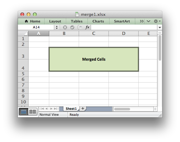
This program is an example of merging cells in a worksheet. See the
merge_range() method for more details.
##############################################################################
#
# A simple example of merging cells with the XlsxWriter Python module.
#
# SPDX-License-Identifier: BSD-2-Clause
# Copyright 2013-2023, John McNamara, jmcnamara@cpan.org
#
import xlsxwriter


# Create an new Excel file and add a worksheet.
workbook = xlsxwriter.Workbook("merge1.xlsx")
worksheet = workbook.add_worksheet()

# Increase the cell size of the merged cells to highlight the formatting.
worksheet.set_column("B:D", 12)
worksheet.set_row(3, 30)
worksheet.set_row(6, 30)
worksheet.set_row(7, 30)


# Create a format to use in the merged range.
merge_format = workbook.add_format(
    {
        "bold": 1,
        "border": 1,
        "align": "center",
        "valign": "vcenter",
        "fg_color": "yellow",
    }
)


# Merge 3 cells.
worksheet.merge_range("B4:D4", "Merged Range", merge_format)

# Merge 3 cells over two rows.
worksheet.merge_range("B7:D8", "Merged Range", merge_format)


workbook.close()
В материале рассказывается о методах модуля openpyxl, которые отвечают за такие свойства электронной таблицы как объединение/разъединение ячеек таблицы, а также особенности стилизации объединенных ячеек.
Содержание:
- Объединение/слияние нескольких ячеек и их разъединение модулем
openpyxl. - Оформление/стилизация разъединенных ячеек модулем
openpyxl.
Объединение/слияние нескольких ячеек и их разъединение.
Модуль openpyxl поддерживает слияние/объединение нескольких ячеек, что очень удобно при записи в них текста, с последующим выравниванием. При слиянии/объединении ячеек, все ячейки, кроме верхней левой, удаляются с рабочего листа. Для переноса информации о границах объединенной ячейки, граничные ячейки объединенной ячейки, создаются как ячейки слияния, которые всегда имеют значение None.
Информацию о форматировании объединенных ячеек смотрите ниже, в подразделе «Оформление объединенных ячеек«.
Пример слияния/объединения ячеек с модулем openpyxl:
>>> from openpyxl import Workbook
>>> wb = Workbook()
>>> ws = wb.active
# объединить ячейки, находящиеся
# в диапазоне `B2 : E2`
>>> ws.merge_cells('B2:E2')
# записываем текст в оставшуюся
# после объединения ячейку 'B2'
>>> ws['B2'] = 'Объединенные ячейки `B2 : E2`'
# сохраняем документ и смотрим что получилось
>>> wb.save("merge.xlsx")
При открытии сохраненного документа и перехода по любой ячейки из диапазона 'B2:E2' видно, что этот диапазон ячеек стал единым. Дополнительно исчезла возможность добавить значения к другим ячейкам этого диапазона.
Теперь разъединим ячейки, которые были объединены ранее, для этого загрузим сохраненный документ.
Пример разъединения ячеек с модулем openpyxl:
>>> from openpyxl import load_workbook
# загружаем сохраненный документ
>>> wb = load_workbook(filename = 'merge.xlsx')
>>> ws = wb.active
# теперь разъединим ячейки,
# в диапазоне `B2 : E2`
>>> ws.unmerge_cells('B2:E2')
# сохраняем документ и смотрим что получилось
>>> wb.save("merge.xlsx")
При открытии сохраненного документа и перехода по любой ячейки из диапазона 'B2:E2' видно, что текст, записанный ранее в ячейку 'B2' принадлежит только ей. Дополнительно появилась возможность добавить значения к другим ячейкам диапазона 'B2:E2'.
Методы слияния ws.merge_cells() и разъединения ws.unmerge_cells() ячеек, кроме диапазона/среза ячеек могут принимать аргументы:
start_row: строка, с которой начинается слияние/разъединение.start_column: колонка, с которой начинается слияние/разъединение.end_row: строка, которой заканчивается слияние/разъединение.end_column: колонка, которой заканчивается слияние/разъединение.
Пример:
# объединение ячеек
>>> ws.merge_cells(start_row=2, start_column=2, end_row=4, end_column=6)
# посмотрите что получилось
>>> wb.save("merge.xlsx")
# и разъединение ячеек
>>> ws.unmerge_cells(start_row=2, start_column=2, end_row=4, end_column=6)
Оформление/стилизация разъединенных ячеек модулем openpyxl.
Объединенная ячейка ведет себя аналогично другим объектам ячеек. Различие заключается лишь в том, что ее значение и формат записываются в левой верхней ячейке. Чтобы изменить, например, границу всей объединенной ячейки, необходимо изменить границу ее левой верхней ячейки.
Пример форматирования объединенной ячейки:
>>> from openpyxl import Workbook
>>> from openpyxl.styles import Border, Side, PatternFill, Font, Alignment
>>> wb = Workbook()
>>> ws = wb.active
# объединим ячейки в диапазоне `B2:E2`
>>> ws.merge_cells('B2:E2')
# в данном случае крайняя верхняя-левая ячейка это `B2`
>>> megre_cell = ws['B2']
# запишем в нее текст
>>> megre_cell.value = 'Объединенные ячейки `B2 : E2`'
# установить высоту строки
>>> ws.row_dimensions[2].height = 30
# установить ширину столбца
>>> ws.column_dimensions['B'].width = 40
# определим стили границ
>>> thins = Side(border_style="thin", color="0000ff")
>>> double = Side(border_style="double", color="ff0000")
# НАЧИНАЕМ ФОРМАТИРОВАНИЕ:
# границы объединенной ячейки
>>> megre_cell.border = Border(top=double, left=thins, right=thins, bottom=double)
# заливка ячейки
>>> megre_cell.fill = PatternFill("solid", fgColor="DDDDDD")
# шрифт ячейки
>>> megre_cell.font = Font(bold=True, color="FF0000", name='Arial', size=14)
# выравнивание текста
>>> megre_cell.alignment = Alignment(horizontal="center", vertical="center")
# сохраняем и смотрим что получилось
>>> wb.save("styled_megre.xlsx")
Дополнительно смотрите:
- Оформление/стилизация ячеек документа XLSX модулем
openpyxl. - Изменение размеров строки/столбца модулем
openpyxl.
I want to merge several series of cell ranges in an Excel file using Python Xlsxwriter, I found the Python command in the Xlsxwriter documentation in this website
http://xlsxwriter.readthedocs.org/en/latest/example_merge1.html
as below:
worksheet.merge_range('B4:D4')
The only problem is that I have my ranges in row and columns numbers format for example (0,0) which is equal to A1. But Xlsxwriter seems to only accept format like A1. I was wondering if anybody else had the same problem and if there is any solution for that.
![]()
jmcnamara
37k6 gold badges86 silver badges105 bronze badges
asked Nov 10, 2014 at 6:19
![]()
2
Almost all methods in XlsxWriter support both A1 and (row, col) notation, see the docs. So the following are equivalent for merge_range():
worksheet.merge_range('B4:D4',    'Merged Range', merge_format)
worksheet.merge_range(3, 1, 3, 3, 'Merged Range', merge_format)
answered Nov 10, 2014 at 9:09
![]()
jmcnamarajmcnamara
37k6 gold badges86 silver badges105 bronze badges
2
В материале рассказывается о методах модуля openpyxl , которые отвечают за такие свойства электронной таблицы как объединение/разъединение ячеек таблицы, а также особенности стилизации объединенных ячеек.
Модуль openpyxl поддерживает слияние/объединение нескольких ячеек, что очень удобно при записи в них текста, с последующим выравниванием. При слиянии/объединении ячеек, все ячейки, кроме верхней левой, удаляются с рабочего листа. Для переноса информации о границах объединенной ячейки, граничные ячейки объединенной ячейки, создаются как ячейки слияния, которые всегда имеют значение None .
Информацию о форматировании объединенных ячеек смотрите ниже, в подразделе «Оформление объединенных ячеек«.
При открытии сохраненного документа и перехода по любой ячейки из диапазона ‘B2:E2’ видно, что этот диапазон ячеек стал единым. Дополнительно исчезла возможность добавить значения к другим ячейкам этого диапазона.
Теперь разъединим ячейки, которые были объединены ранее, для этого загрузим сохраненный документ.
При открытии сохраненного документа и перехода по любой ячейки из диапазона ‘B2:E2’ видно, что текст, записанный ранее в ячейку ‘B2’ принадлежит только ей. Дополнительно появилась возможность добавить значения к другим ячейкам диапазона ‘B2:E2’ .
Методы слияния ws.merge_cells() и разъединения ws.unmerge_cells() ячеек, кроме диапазона/среза ячеек могут принимать аргументы:
Объединенная ячейка ведет себя аналогично другим объектам ячеек. Различие заключается лишь в том, что ее значение и формат записываются в левой верхней ячейке. Чтобы изменить, например, границу всей объединенной ячейки, необходимо изменить границу ее левой верхней ячейки.
EasyXLS Excel library can be used to export Excel files with Python on Windows, Linux, Mac or other operating systems. The integration vary depending on the operating system or if the bridge for .NET Framework of Java is chosen:
If you opt for the .NET version of EasyXLS, the below code requires Pythonnet, a bridge between Python and .NET Framework.
If you already own a license key, you may login and download EasyXLS from your account.
Install the downloaded EasyXLS installer for v8.6 or earlier.
For the installation you need to run «pip» command as it follows. Pip is a package-management system used to install and manage software packages written in Python.
EasyXLS.dll must be added to your project. EasyXLS.dll can be found:
— Inside the downloaded archive at Step 1 for EasyXLS v9.0 or later
— Under installation path for EasyXLS v8.6 or earlier, in «Dot NET version» folder.
Execute the following Python code that exports an Excel file with merge cells.
If you opt for the Java version of EasyXLS, a similar code as above requires Py4J, Pyjnius or any other bridge between Python and Java.
If you already own a license key, you may login and download EasyXLS from your account.
Install the downloaded EasyXLS installer for v8.6 or earlier.
For the Py4j installation you need to run «pip» command as it follows. Pip is a package-management system used to install and manage software packages written in Python.
The following Java code needs to be running in the background prior to executing the Python code.
py4j.jar must be added to your classpath of the additional Java program. py4j.jar can be found after installing Py4j, in «
Step 5: Add EasyXLS library to CLASSPATH
EasyXLS.jar must be added to your classpath of the additional Java program. EasyXLS.jar can be found:
— Inside the downloaded archive at Step 1 for EasyXLS v9.0 or later
— Under installation path for EasyXLS v8.6 or earlier, in «Lib» folder.
Step 6: Run additional Java program
Start the gateway server application and it will implicitly start Java Virtual Machine as well.
Step 7: Run Python code that merges cells in Excel sheet
Execute a code as below Python code that exports an Excel file with merge cells.
Источник
Working with Excel Spreadsheets in Python
You all must have worked with Excel at some time in your life and must have felt the need for automating some repetitive or tedious task. Don’t worry in this tutorial we are going to learn about how to work with Excel using Python, or automating Excel using Python. We will be covering this with the help of the Openpyxl module.
Getting Started
Openpyxl is a Python library that provides various methods to interact with Excel Files using Python. It allows operations like reading, writing, arithmetic operations, plotting graphs, etc.
This module does not come in-built with Python. To install this type the below command in the terminal.
Reading from Spreadsheets
To read an Excel file you have to open the spreadsheet using the load_workbook() method. After that, you can use the active to select the first sheet available and the cell attribute to select the cell by passing the row and column parameter. The value attribute prints the value of the particular cell. See the below example to get a better understanding.
Note: The first row or column integer is 1, not 0.
Dataset Used: It can be downloaded from here.
Example:
Python3
Output:
Reading from Multiple Cells
There can be two ways of reading from multiple cells.
Method 1: We can get the count of the total rows and columns using the max_row and max_column respectively. We can use these values inside the for loop to get the value of the desired row or column or any cell depending upon the situation. Let’s see how to get the value of the first column and first row.
Example:
Python3
Output:
Method 2: We can also read from multiple cells using the cell name. This can be seen as the list slicing of Python.
Python3
Output:
Refer to the below article to get detailed information about reading excel files using openpyxl.
Writing to Spreadsheets
First, let’s create a new spreadsheet, and then we will write some data to the newly created file. An empty spreadsheet can be created using the Workbook() method. Let’s see the below example.
Example:
Python3
Output:
![]()
After creating an empty file, let’s see how to add some data to it using Python. To add data first we need to select the active sheet and then using the cell() method we can select any particular cell by passing the row and column number as its parameter. We can also write using cell names. See the below example for a better understanding.
Example:
Python3
Output:
Refer to the below article to get detailed information about writing to excel.
Appending to the Spreadsheet
In the above example, you will see that every time you try to write to a spreadsheet the existing data gets overwritten, and the file is saved as a new file. This happens because the Workbook() method always creates a new workbook file object. To write to an existing workbook you must open the file with the load_workbook() method. We will use the above-created workbook.
Example:
Python3
Output:
We can also use the append() method to append multiple data at the end of the sheet.
Example:
Python3
Output:
Arithmetic Operation on Spreadsheet
Arithmetic operations can be performed by typing the formula in a particular cell of the spreadsheet. For example, if we want to find the sum then =Sum() formula of the excel file is used.
Example:
Python3
Output:
Refer to the below article to get detailed information about the Arithmetic operations on Spreadsheet.
Adjusting Rows and Column
Worksheet objects have row_dimensions and column_dimensions attributes that control row heights and column widths. A sheet’s row_dimensions and column_dimensions are dictionary-like values; row_dimensions contains RowDimension objects and column_dimensions contains ColumnDimension objects. In row_dimensions, one can access one of the objects using the number of the row (in this case, 1 or 2). In column_dimensions, one can access one of the objects using the letter of the column (in this case, A or B).
Источник
The Worksheet Class
The worksheet class represents an Excel worksheet. It handles operations such as writing data to cells or formatting worksheet layout.
A worksheet object isn’t instantiated directly. Instead a new worksheet is created by calling the add_worksheet() method from a Workbook() object:
XlsxWriter supports Excels worksheet limits of 1,048,576 rows by 16,384 columns.
worksheet.write()
Write generic data to a worksheet cell.
-1: Row or column is out of worksheet bounds.
Other values from the called write methods.
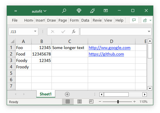
Excel makes a distinction between data types such as strings, numbers, blanks, formulas and hyperlinks. To simplify the process of writing data to an XlsxWriter file the write() method acts as a general alias for several more specific methods:
The rules for handling data in write() are as follows:
- Data types float , int , long , decimal.Decimal and fractions.Fraction are written using write_number() .
- Data types datetime.datetime , datetime.datedatetime.time or datetime.timedelta are written using write_datetime() .
- None and empty strings «» are written using write_blank() .
- Data type bool is written using write_boolean() .
Strings are then handled as follows:
- Strings that start with «=» are assumed to match a formula and are written using write_formula() . This can be overridden, see below.
- Strings that match supported URL types are written using write_url() . This can be overridden, see below.
- When the Workbook() constructor strings_to_numbers option is True strings that convert to numbers using float() are written using write_number() in order to avoid Excel warnings about “Numbers Stored as Text”. See the note below.
- Strings that don’t match any of the above criteria are written using write_string() .
If none of the above types are matched the value is evaluated with float() to see if it corresponds to a user defined float type. If it does then it is written using write_number() .
Finally, if none of these rules are matched then a TypeError exception is raised. However, it is also possible to handle additional, user defined, data types using the add_write_handler() method explained below and in Writing user defined types .
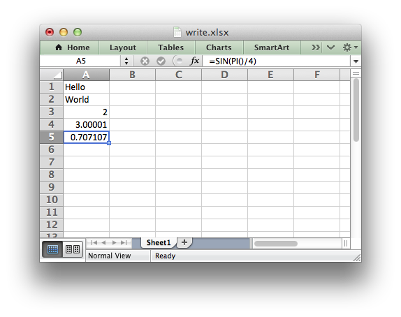
Here are some examples:
This creates a worksheet like the following:
The Workbook() constructor option takes three optional arguments that can be used to override string handling in the write() function. These options are shown below with their default values:
The write() method supports two forms of notation to designate the position of cells: Row-column notation and A1 notation:
The cell_format parameter in the sub write methods is used to apply formatting to the cell. This parameter is optional but when present it should be a valid Format object:
worksheet.add_write_handler()
Add a callback function to the write() method to handle user define types.
| Parameters: |
|
|---|---|
| Returns: |
| Parameters: |
|
|---|
As explained above, the write() method maps basic Python types to corresponding Excel types. If you want to write an unsupported type then you can either avoid write() and map the user type in your code to one of the more specific write methods or you can extend it using the add_write_handler() method.
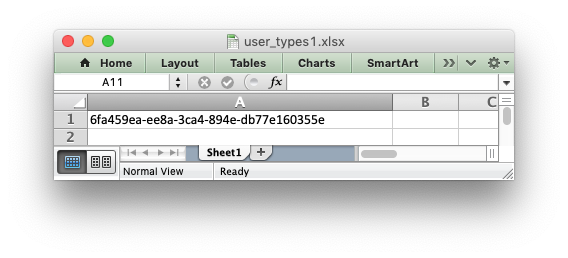
For example, say you wanted to automatically write uuid values as strings using write() you would start by creating a function that takes the uuid, converts it to a string and then writes it using write_string() :
You could then add a handler that matches the uuid type and calls your user defined function:
Then you can use write() without further modification:
Multiple callback functions can be added using add_write_handler() but only one callback action is allowed per type. However, it is valid to use the same callback function for different types:
See Writing user defined types for more details on how this feature works and how to write callback functions, and also the following examples:
worksheet.write_string()
Write a string to a worksheet cell.
-1: Row or column is out of worksheet bounds.
-2: String truncated to 32k characters.
The write_string() method writes a string to the cell specified by row and column :
Both row-column and A1 style notation are supported, as shown above. See Working with Cell Notation for more details.
The cell_format parameter is used to apply formatting to the cell. This parameter is optional but when present is should be a valid Format object.
Unicode strings are supported in UTF-8 encoding. This generally requires that your source file is UTF-8 encoded:
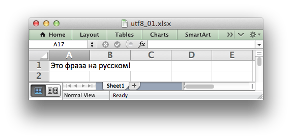
Alternatively, you can read data from an encoded file, convert it to UTF-8 during reading and then write the data to an Excel file. See Example: Unicode — Polish in UTF-8 and Example: Unicode — Shift JIS .
The maximum string size supported by Excel is 32,767 characters. Strings longer than this will be truncated by write_string() .
Even though Excel allows strings of 32,767 characters it can only display 1000 in a cell. However, all 32,767 characters are displayed in the formula bar.
worksheet.write_number()
Write a number to a worksheet cell.
| Parameters: |
|
|---|---|
| Returns: |
-1: Row or column is out of worksheet bounds.
The write_number() method writes numeric types to the cell specified by row and column :
Both row-column and A1 style notation are supported, as shown above. See Working with Cell Notation for more details.
The numeric types supported are float , int , long , decimal.Decimal and fractions.Fraction or anything that can be converted via float() .
When written to an Excel file numbers are converted to IEEE-754 64-bit double-precision floating point. This means that, in most cases, the maximum number of digits that can be stored in Excel without losing precision is 15.
NAN and INF are not supported and will raise a TypeError exception unless the nan_inf_to_errors Workbook() option is used.
The cell_format parameter is used to apply formatting to the cell. This parameter is optional but when present is should be a valid Format object.
worksheet.write_formula()
Write a formula to a worksheet cell.
| Parameters: |
|
|---|---|
| Returns: |
-1: Row or column is out of worksheet bounds.
The write_formula() method writes a formula or function to the cell specified by row and column :
Both row-column and A1 style notation are supported, as shown above. See Working with Cell Notation for more details.
Array formulas are also supported:
See also the write_array_formula() method below.
The cell_format parameter is used to apply formatting to the cell. This parameter is optional but when present is should be a valid Format object.
If required, it is also possible to specify the calculated result of the formula using the optional value parameter. This is occasionally necessary when working with non-Excel applications that don’t calculate the result of the formula:
See Formula Results for more details.
Excel stores formulas in US style formatting regardless of the Locale or Language of the Excel version:
Excel 2010 and 2013 added functions which weren’t defined in the original file specification. These functions are referred to as future functions. Examples of these functions are ACOT , CHISQ.DIST.RT , CONFIDENCE.NORM , STDEV.P , STDEV.S and WORKDAY.INTL . In XlsxWriter these require a prefix:
See Formulas added in Excel 2010 and later for a detailed explanation and full list of functions that are affected.
worksheet.write_array_formula()
Write an array formula to a worksheet cell.
| Parameters: |
|
|---|---|
| Returns: |
-1: Row or column is out of worksheet bounds.
The write_array_formula() method writes an array formula to a cell range. In Excel an array formula is a formula that performs a calculation on a set of values. It can return a single value or a range of values.
An array formula is indicated by a pair of braces around the formula: <=SUM(A1:B1*A2:B2)>.
For array formulas that return a range of values you must specify the range that the return values will be written to:
Both row-column and A1 style notation are supported, as shown above. See Working with Cell Notation for more details.
If the array formula returns a single value then the first_ and last_ parameters should be the same:
It this case however it is easier to just use the write_formula() or write() methods:
The cell_format parameter is used to apply formatting to the cell. This parameter is optional but when present is should be a valid Format object.
If required, it is also possible to specify the calculated result of the formula (see discussion of formulas and the value parameter for the write_formula() method above). However, using this parameter only writes a single value to the upper left cell in the result array. See Formula Results for more details.
worksheet.write_dynamic_array_formula()
Write an array formula to a worksheet cell.
| Parameters: |
|
|---|---|
| Returns: |
-1: Row or column is out of worksheet bounds.
The write_dynamic_array_formula() method writes an dynamic array formula to a cell range. Dynamic array formulas are explained in detail in Dynamic Array support .
The syntax of write_dynamic_array_formula() is the same as write_array_formula() , shown above, except that you don’t need to add <> braces:
Which gives the following result:
It is also possible to specify the first cell of the range to get the same results:
worksheet.write_blank()
Write a blank worksheet cell.
| Parameters: |
|
|---|---|
| Returns: |
-1: Row or column is out of worksheet bounds.
Write a blank cell specified by row and column :
Both row-column and A1 style notation are supported, as shown above. See Working with Cell Notation for more details.
This method is used to add formatting to a cell which doesn’t contain a string or number value.
Excel differentiates between an “Empty” cell and a “Blank” cell. An “Empty” cell is a cell which doesn’t contain data or formatting whilst a “Blank” cell doesn’t contain data but does contain formatting. Excel stores “Blank” cells but ignores “Empty” cells.
As such, if you write an empty cell without formatting it is ignored:
This seemingly uninteresting fact means that you can write arrays of data without special treatment for None or empty string values.
worksheet.write_boolean()
Write a boolean value to a worksheet cell.
| Parameters: |
|
|---|---|
| Returns: |
-1: Row or column is out of worksheet bounds.
The write_boolean() method writes a boolean value to the cell specified by row and column :
Both row-column and A1 style notation are supported, as shown above. See Working with Cell Notation for more details.
The cell_format parameter is used to apply formatting to the cell. This parameter is optional but when present is should be a valid Format object.
worksheet.write_datetime()
Write a date or time to a worksheet cell.
| Parameters: |
|
|---|---|
| Returns: |
-1: Row or column is out of worksheet bounds.
The write_datetime() method can be used to write a date or time to the cell specified by row and column :
Both row-column and A1 style notation are supported, as shown above. See Working with Cell Notation for more details.
The datetime should be a datetime.datetime , datetime.date datetime.time or datetime.timedelta object. The datetime class is part of the standard Python libraries.
There are many ways to create datetime objects, for example the datetime.datetime.strptime() method:
See the datetime documentation for other date/time creation methods.
A date/time should have a cell_format of type Format , otherwise it will appear as a number:
If required, a default date format string can be set using the Workbook() constructor default_date_format option.
worksheet.write_url()
Write a hyperlink to a worksheet cell.
| Parameters: |
|
|---|---|
| Returns: |
-1: Row or column is out of worksheet bounds.
-2: String longer than 32k characters.
-3: Url longer than Excel limit of 2079 characters.
-4: Exceeds Excel limit of 65,530 urls per worksheet.
The write_url() method is used to write a hyperlink in a worksheet cell. The url is comprised of two elements: the displayed string and the non-displayed link. The displayed string is the same as the link unless an alternative string is specified:
Both row-column and A1 style notation are supported, as shown above. See Working with Cell Notation for more details.
The cell_format parameter is used to apply formatting to the cell. This parameter is optional and the default Excel hyperlink style will be used if it isn’t specified. If required you can access the default url format using the Workbook get_default_url_format() method:
Four web style URI’s are supported: http:// , https:// , ftp:// and mailto: :
All of the these URI types are recognized by the write() method, so the following are equivalent:
You can display an alternative string using the string parameter:
If you wish to have some other cell data such as a number or a formula you can overwrite the cell using another call to write_*() :
There are two local URIs supported: internal: and external: . These are used for hyperlinks to internal worksheet references or external workbook and worksheet references:
Worksheet references are typically of the form Sheet1!A1 . You can also link to a worksheet range using the standard Excel notation: Sheet1!A1:B2 .
In external links the workbook and worksheet name must be separated by the # character: external:Workbook.xlsx#Sheet1!A1′ .
You can also link to a named range in the target worksheet. For example say you have a named range called my_name in the workbook c:tempfoo.xlsx you could link to it as follows:
Excel requires that worksheet names containing spaces or non alphanumeric characters are single quoted as follows ‘Sales Data’!A1 .
Links to network files are also supported. Network files normally begin with two back slashes as follows \NETWORKetc . In order to generate this in a single or double quoted string you will have to escape the backslashes, ‘\\NETWORK\etc’ or use a raw string r’\NETWORKetc’ .
Alternatively, you can avoid most of these quoting problems by using forward slashes. These are translated internally to backslashes:
XlsxWriter will escape the following characters in URLs as required by Excel: s » > [ ] ` ^ < >unless the URL already contains %xx style escapes. In which case it is assumed that the URL was escaped correctly by the user and will by passed directly to Excel.
Versions of Excel prior to Excel 2015 limited hyperlink links and anchor/locations to 255 characters each. Versions after that support urls up to 2079 characters. XlsxWriter versions >= 1.2.3 support this longer limit by default. However, a lower or user defined limit can be set via the max_url_length property in the Workbook() constructor.
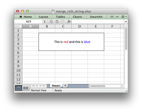
worksheet.write_rich_string()
Write a “rich” string with multiple formats to a worksheet cell.
| Parameters: |
|
|---|---|
| Returns: |
-1: Row or column is out of worksheet bounds.
-2: String longer than 32k characters.
-3: 2 consecutive formats used.
-4: Empty string used.
-5: Insufficient parameters.
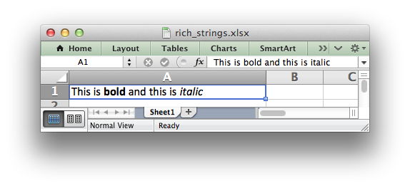
The write_rich_string() method is used to write strings with multiple formats. For example to write the string “This is bold and this is italic” you would use the following:
Both row-column and A1 style notation are supported. The following are equivalent:
The basic rule is to break the string into fragments and put a Format object before the fragment that you want to format. For example:
String fragments that don’t have a format are given a default format. So for example when writing the string “Some bold text” you would use the first example below but it would be equivalent to the second:
If you have formats and segments in a list you can add them like this, using the standard Python list unpacking syntax:
In Excel only the font properties of the format such as font name, style, size, underline, color and effects are applied to the string fragments in a rich string. Other features such as border, background, text wrap and alignment must be applied to the cell.
The write_rich_string() method allows you to do this by using the last argument as a cell format (if it is a format object). The following example centers a rich string in the cell:
Excel doesn’t allow the use of two consecutive formats in a rich string or an empty string fragment. For either of these conditions a warning is raised and the input to write_rich_string() is ignored.
Also, the maximum string size supported by Excel is 32,767 characters. If the rich string exceeds this limit a warning is raised and the input to write_rich_string() is ignored.
worksheet.write_row()
Write a row of data starting from (row, col).
| Parameters: |
|
|---|---|
| Returns: |
Other: Error return value of the write() method.
The write_row() method can be used to write a list of data in one go. This is useful for converting the results of a database query into an Excel worksheet. The write() method is called for each element of the data. For example:
Both row-column and A1 style notation are supported. The following are equivalent:
worksheet.write_column()
Write a column of data starting from (row, col).
| Parameters: |
|
|---|---|
| Returns: |
Other: Error return value of the write() method.
The write_column() method can be used to write a list of data in one go. This is useful for converting the results of a database query into an Excel worksheet. The write() method is called for each element of the data. For example:
Both row-column and A1 style notation are supported. The following are equivalent:
worksheet.set_row()
Set properties for a row of cells.
| Parameters: |
|
|---|---|
| Returns: |
-1: Row is out of worksheet bounds.
The set_row() method is used to change the default properties of a row. The most common use for this method is to change the height of a row:
The height is specified in character units. To specify the height in pixels use the set_row_pixels() method.
The other common use for set_row() is to set the Format for all cells in the row:
If you wish to set the format of a row without changing the default row height you can pass None as the height parameter or use the default row height of 15:
The cell_format parameter will be applied to any cells in the row that don’t have a format. As with Excel it is overridden by an explicit cell format. For example:
The options parameter is a dictionary with the following possible keys:
Options can be set as follows:
The ‘hidden’ option is used to hide a row. This can be used, for example, to hide intermediary steps in a complicated calculation:
The ‘level’ parameter is used to set the outline level of the row. Outlines are described in Working with Outlines and Grouping . Adjacent rows with the same outline level are grouped together into a single outline.
The following example sets an outline level of 1 for some rows:
Excel allows up to 7 outline levels. The ‘level’ parameter should be in the range 0 level 7 .
The ‘hidden’ parameter can also be used to hide collapsed outlined rows when used in conjunction with the ‘level’ parameter:
The ‘collapsed’ parameter is used in collapsed outlines to indicate which row has the collapsed ‘+’ symbol:
worksheet.set_row_pixels()
Set properties for a row of cells, with the row height in pixels.
| Parameters: |
|
|---|---|
| Returns: |
-1: Row is out of worksheet bounds.
The set_row_pixels() method is identical to set_row() except that the height can be set in pixels instead of Excel character units:
All other parameters and options are the same as set_row() . See the documentation on set_row() for more details.
worksheet.set_column()
Set properties for one or more columns of cells.
| Parameters: |
|
|---|---|
| Returns: |
-1: Column is out of worksheet bounds.
The set_column() method can be used to change the default properties of a single column or a range of columns:
If set_column() is applied to a single column the value of first_col and last_col should be the same:
It is also possible, and generally clearer, to specify a column range using the form of A1 notation used for columns. See Working with Cell Notation for more details.
The width parameter sets the column width in the same units used by Excel which is: the number of characters in the default font. The default width is 8.43 in the default font of Calibri 11. The actual relationship between a string width and a column width in Excel is complex. See the following explanation of column widths from the Microsoft support documentation for more details. To set the width in pixels use the set_column_pixels() method.
See also the autofit() method for simulated autofitting of column widths.
As usual the cell_format Format parameter is optional. If you wish to set the format without changing the default column width you can pass None as the width parameter:
The cell_format parameter will be applied to any cells in the column that don’t have a format. For example:
A row format takes precedence over a default column format:
The options parameter is a dictionary with the following possible keys:
Options can be set as follows:
The ‘hidden’ option is used to hide a column. This can be used, for example, to hide intermediary steps in a complicated calculation:
The ‘level’ parameter is used to set the outline level of the column. Outlines are described in Working with Outlines and Grouping . Adjacent columns with the same outline level are grouped together into a single outline.
The following example sets an outline level of 1 for columns B to G:
Excel allows up to 7 outline levels. The ‘level’ parameter should be in the range 0 level 7 .
The ‘hidden’ parameter can also be used to hide collapsed outlined columns when used in conjunction with the ‘level’ parameter:
The ‘collapsed’ parameter is used in collapsed outlines to indicate which column has the collapsed ‘+’ symbol:
worksheet.set_column_pixels()
Set properties for one or more columns of cells, with the width in pixels.
| Parameters: |
|
|---|---|
| Returns: |
-1: Column is out of worksheet bounds.
The set_column_pixels() method is identical to set_column() except that the width can be set in pixels instead of Excel character units:
![]()
All other parameters and options are the same as set_column() . See the documentation on set_column() for more details.
worksheet.autofit()
Simulates autofit for column widths.
| Parameters: |
|
|---|---|
| Returns: |
| Returns: | Nothing. |
|---|
The autofit() method can be used to simulate autofitting column widths based on the largest string/number in the column:
There is no option in the xlsx file format that can be used to say “autofit columns on loading”. Auto-fitting of columns is something that Excel does at runtime when it has access to all of the worksheet information as well as the Windows functions for calculating display areas based on fonts and formatting.
The worksheet.autofit() method simulates this behavior by calculating string widths using metrics taken from Excel. As such there are some limitations to be aware of when using this method:
- It is a simulated method and may not be accurate in all cases.
- It is based on the default font and font size of Calibri 11. It will not give accurate results for other fonts or font sizes.
This isn’t perfect but for most cases it should be sufficient and if not you can set your own widths, see below.
The autofit() method won’t override a user defined column width set with set_column() or set_column_pixels() if it is greater than the autofit value. This allows the user to set a minimum width value for a column.
You can also call set_column() and set_column_pixels() after autofit() to override any of the calculated values.
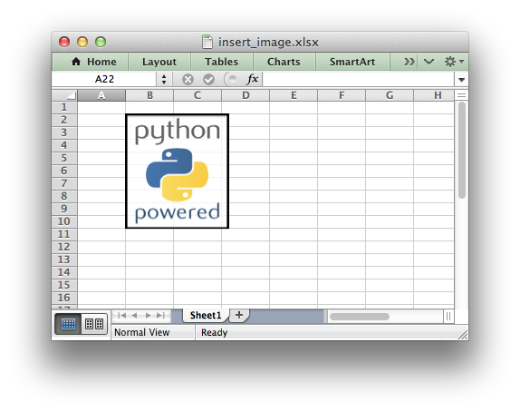
worksheet.insert_image()
Insert an image in a worksheet cell.
-1: Row or column is out of worksheet bounds.
This method can be used to insert a image into a worksheet. The image can be in PNG, JPEG, GIF, BMP, WMF or EMF format (see the notes about BMP and EMF below):
Both row-column and A1 style notation are supported. The following are equivalent:
A file path can be specified with the image name:
The insert_image() method takes optional parameters in a dictionary to position and scale the image. The available parameters with their default values are:
The offset values are in pixels:
The offsets can be greater than the width or height of the underlying cell. This can be occasionally useful if you wish to align two or more images relative to the same cell.
The x_scale and y_scale parameters can be used to scale the image horizontally and vertically:
The url parameter can used to add a hyperlink/url to the image. The tip parameter gives an optional mouseover tooltip for images with hyperlinks:
See also write_url() for details on supported URIs.
The image_data parameter is used to add an in-memory byte stream in io.BytesIO format:
This is generally used for inserting images from URLs:
When using the image_data parameter a filename must still be passed to insert_image() since it is used by Excel as a default description field (see below). However, it can be a blank string if the description isn’t required. In the previous example the filename/description is extracted from the URL string. See also Example: Inserting images from a URL or byte stream into a worksheet .
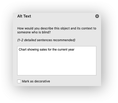
The description field can be used to specify a description or “alt text” string for the image. In general this would be used to provide a text description of the image to help accessibility. It is an optional parameter and defaults to the filename of the image. It can be used as follows:

The optional decorative parameter is also used to help accessibility. It is used to mark the image as decorative, and thus uninformative, for automated screen readers. As in Excel, if this parameter is in use the description field isn’t written. It is used as follows:
The object_position parameter can be used to control the object positioning of the image:
Where object_position has the following allowable values:
- Move and size with cells.
- Move but don’t size with cells (the default).
- Don’t move or size with cells.
- Same as Option 1 to “move and size with cells” except XlsxWriter applies hidden cells after the image is inserted.
See Working with Object Positioning for more detailed information about the positioning and scaling of images within a worksheet.
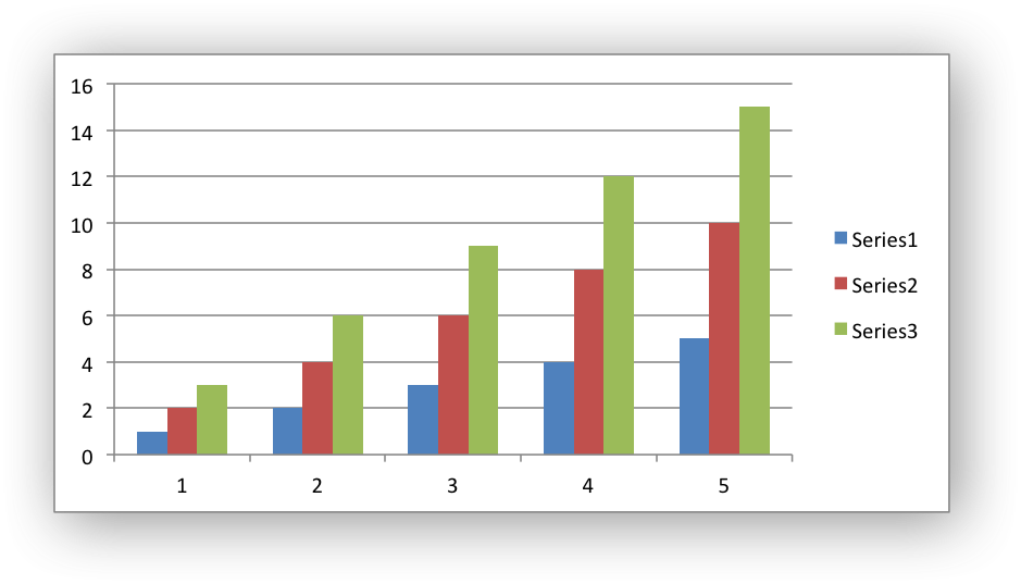
worksheet.insert_chart()
Write a string to a worksheet cell.
| Parameters: |
|
|---|---|
| Returns: |
-1: Row or column is out of worksheet bounds.
This method can be used to insert a chart into a worksheet. A chart object is created via the Workbook add_chart() method where the chart type is specified:
It is then inserted into a worksheet as an embedded chart:
A chart can only be inserted into a worksheet once. If several similar charts are required then each one must be created separately with add_chart() .
Both row-column and A1 style notation are supported. The following are equivalent:
The insert_chart() method takes optional parameters in a dictionary to position and scale the chart. The available parameters with their default values are:
The offset values are in pixels:
The x_scale and y_scale parameters can be used to scale the chart horizontally and vertically:
These properties can also be set via the Chart set_size() method.
The description field can be used to specify a description or “alt text” string for the chart. In general this would be used to provide a text description of the chart to help accessibility. It is an optional parameter and has no default. It can be used as follows:
The optional decorative parameter is also used to help accessibility. It is used to mark the chart as decorative, and thus uninformative, for automated screen readers. As in Excel, if this parameter is in use the description field isn’t written. It is used as follows:
The object_position parameter can be used to control the object positioning of the chart:
Where object_position has the following allowable values:
- Move and size with cells (the default).
- Move but don’t size with cells.
- Don’t move or size with cells.
See Working with Object Positioning for more detailed information about the positioning and scaling of charts within a worksheet.
worksheet.insert_textbox()
Write a string to a worksheet cell.
| Parameters: |
|
|---|---|
| Returns: |
-1: Row or column is out of worksheet bounds.
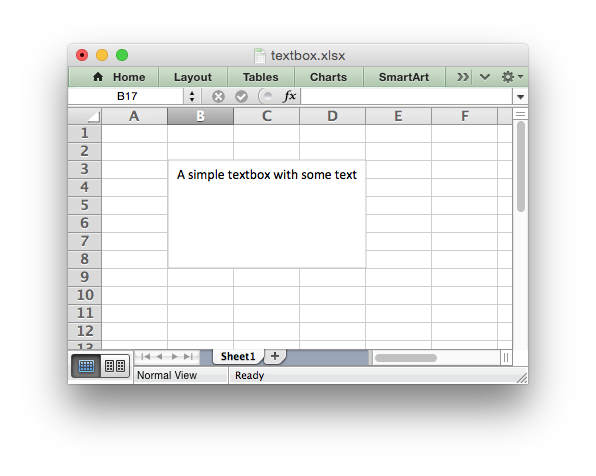
This method can be used to insert a textbox into a worksheet:
Both row-column and A1 style notation are supported. The following are equivalent:
The size and formatting of the textbox can be controlled via the options dict:
These options are explained in more detail in the Working with Textboxes section.
See Working with Object Positioning for more detailed information about the positioning and scaling of images within a worksheet.
worksheet.insert_button()
Insert a VBA button control on a worksheet.
| Parameters: |
|
|---|---|
| Returns: |
-1: Row or column is out of worksheet bounds.
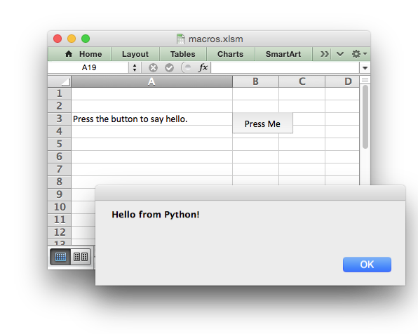
The insert_button() method can be used to insert an Excel form button into a worksheet.
This method is generally only useful when used in conjunction with the Workbook add_vba_project() method to tie the button to a macro from an embedded VBA project:
Both row-column and A1 style notation are supported. The following are equivalent:
The insert_button() method takes optional parameters in a dictionary to position and scale the chart. The available parameters with their default values are:
The macro option is used to set the macro that the button will invoke when the user clicks on it. The macro should be included using the Workbook add_vba_project() method shown above.
The caption is used to set the caption on the button. The default is Button n where n is the button number.
The default button width is 64 pixels which is the width of a default cell and the default button height is 20 pixels which is the height of a default cell.
The offset, scale and description options are the same as for insert_chart() , see above.
worksheet.data_validation()
Write a conditional format to range of cells.
| Parameters: |
|
|---|---|
| Returns: |
-1: Row or column is out of worksheet bounds.
-2: Incorrect parameter or option.
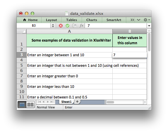
The data_validation() method is used to construct an Excel data validation or to limit the user input to a dropdown list of values:
The data validation can be applied to a single cell or a range of cells. As usual you can use A1 or Row/Column notation, see Working with Cell Notation :
With Row/Column notation you must specify all four cells in the range: (first_row, first_col, last_row, last_col) . If you need to refer to a single cell set the last_ values equal to the first_ values. With A1 notation you can refer to a single cell or a range of cells:
The options parameter in data_validation() must be a dictionary containing the parameters that describe the type and style of the data validation. There are a lot of available options which are described in detail in a separate section: Working with Data Validation . See also Example: Data Validation and Drop Down Lists .
worksheet.conditional_format()
Write a conditional format to range of cells.
| Parameters: |
|
|---|---|
| Returns: |
-1: Row or column is out of worksheet bounds.
-2: Incorrect parameter or option.
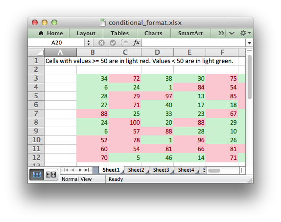
The conditional_format() method is used to add formatting to a cell or range of cells based on user defined criteria:
The conditional format can be applied to a single cell or a range of cells. As usual you can use A1 or Row/Column notation, see Working with Cell Notation :
With Row/Column notation you must specify all four cells in the range: (first_row, first_col, last_row, last_col) . If you need to refer to a single cell set the last_ values equal to the first_ values. With A1 notation you can refer to a single cell or a range of cells:
The options parameter in conditional_format() must be a dictionary containing the parameters that describe the type and style of the conditional format. There are a lot of available options which are described in detail in a separate section: Working with Conditional Formatting . See also Example: Conditional Formatting .
worksheet.add_table()
Add an Excel table to a worksheet.
| Parameters: |
|
|---|---|
| Returns: |
OverlappingRange – if the range overlaps a previous merge or table range.
-1: Row or column is out of worksheet bounds.
-2: Incorrect parameter or option.
-3: Not supported in constant_memory mode.
The add_table() method is used to group a range of cells into an Excel Table:
This method contains a lot of parameters and is described in Working with Worksheet Tables .
Both row-column and A1 style notation are supported. The following are equivalent:
Tables aren’t available in XlsxWriter when Workbook() ‘constant_memory’ mode is enabled.
worksheet.add_sparkline()
| Parameters: |
|
|---|---|
| Raises: |
-1: Row or column is out of worksheet bounds.
-2: Incorrect parameter or option.
Sparklines are small charts that fit in a single cell and are used to show trends in data.
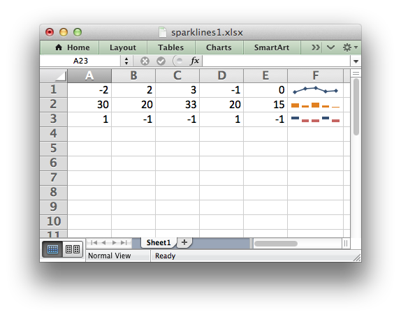
The add_sparkline() worksheet method is used to add sparklines to a cell or a range of cells:
Both row-column and A1 style notation are supported. The following are equivalent:
This method contains a lot of parameters and is described in detail in Working with Sparklines .
Sparklines are a feature of Excel 2010+ only. You can write them to an XLSX file that can be read by Excel 2007 but they won’t be displayed.
Write a comment to a worksheet cell.
| Parameters: |
|
|---|---|
| Returns: |
-1: Row or column is out of worksheet bounds.
-2: String longer than 32k characters.
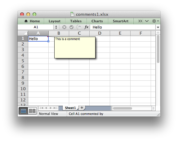
The write_comment() method is used to add a comment to a cell. A comment is indicated in Excel by a small red triangle in the upper right-hand corner of the cell. Moving the cursor over the red triangle will reveal the comment.
The following example shows how to add a comment to a cell:
Both row-column and A1 style notation are supported. The following are equivalent:
The properties of the cell comment can be modified by passing an optional dictionary of key/value pairs to control the format of the comment. For example:
Most of these options are quite specific and in general the default comment behavior will be all that you need. However, should you need greater control over the format of the cell comment the following options are available:
Make any comments in the worksheet visible.
This method is used to make all cell comments visible when a worksheet is opened:
Individual comments can be made visible using the visible parameter of the write_comment method (see above):
If all of the cell comments have been made visible you can hide individual comments as follows:
Set the default author of the cell comments.
| Parameters: |
|
|---|---|
| Returns: |
| Parameters: | author (string) – Comment author. |
|---|
This method is used to set the default author of all cell comments:
Individual comment authors can be set using the author parameter of the write_comment method (see above).
If no author is specified the default comment author name is an empty string.
worksheet.get_name()
Retrieve the worksheet name.
The get_name() method is used to retrieve the name of a worksheet. This is something useful for debugging or logging:
There is no set_name() method. The only safe way to set the worksheet name is via the add_worksheet() method.
worksheet.activate()
Make a worksheet the active, i.e., visible worksheet.
The activate() method is used to specify which worksheet is initially visible in a multi-sheet workbook:
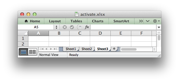
More than one worksheet can be selected via the select() method, see below, however only one worksheet can be active.
The default active worksheet is the first worksheet.
worksheet.select()
Set a worksheet tab as selected.
The select() method is used to indicate that a worksheet is selected in a multi-sheet workbook:
A selected worksheet has its tab highlighted. Selecting worksheets is a way of grouping them together so that, for example, several worksheets could be printed in one go. A worksheet that has been activated via the activate() method will also appear as selected.
worksheet.hide()
Hide the current worksheet.
The hide() method is used to hide a worksheet:
You may wish to hide a worksheet in order to avoid confusing a user with intermediate data or calculations.
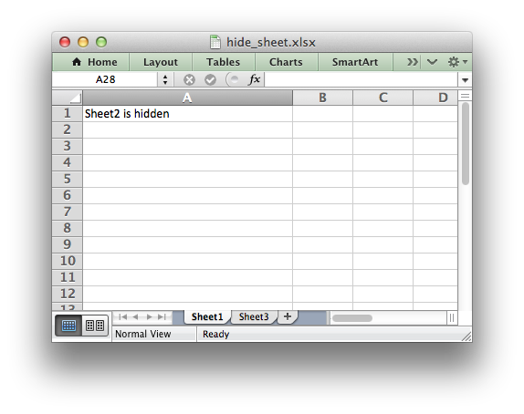
A hidden worksheet can not be activated or selected so this method is mutually exclusive with the activate() and select() methods. In addition, since the first worksheet will default to being the active worksheet, you cannot hide the first worksheet without activating another sheet:
worksheet.set_first_sheet()
Set current worksheet as the first visible sheet tab.
The activate() method determines which worksheet is initially selected. However, if there are a large number of worksheets the selected worksheet may not appear on the screen. To avoid this you can select which is the leftmost visible worksheet tab using set_first_sheet() :
This method is not required very often. The default value is the first worksheet.
worksheet.merge_range()
Merge a range of cells.
OverlappingRange – if the range overlaps a previous merge or table range.
-1: Row or column is out of worksheet bounds.
Other: Error return value of the called write() method.
The merge_range() method allows cells to be merged together so that they act as a single area.
Excel generally merges and centers cells at same time. To get similar behavior with XlsxWriter you need to apply a Format :
Both row-column and A1 style notation are supported. The following are equivalent:
It is possible to apply other formatting to the merged cells as well:
The merge_range() method writes its data argument using write() . Therefore it will handle numbers, strings and formulas as usual. If this doesn’t handle your data correctly then you can overwrite the first cell with a call to one of the other write_*() methods using the same Format as in the merged cells. See Example: Merging Cells with a Rich String .
Merged ranges generally don’t work in XlsxWriter when Workbook() ‘constant_memory’ mode is enabled.
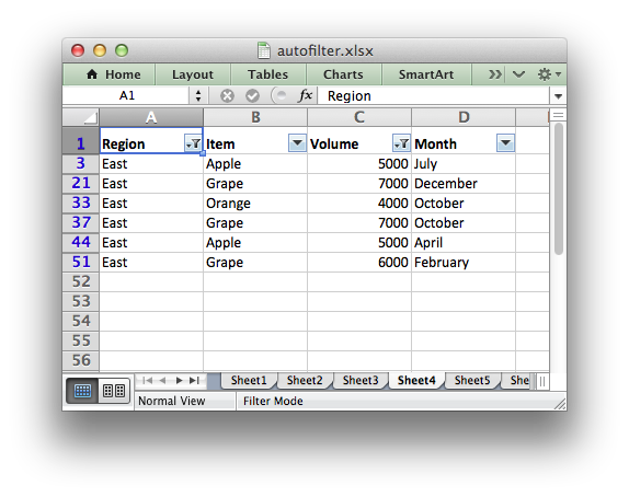
worksheet.autofilter()
Set the autofilter area in the worksheet.
| Parameters: |
|
|---|---|
| Raises: |
| Parameters: |
|
|---|
The autofilter() method allows an autofilter to be added to a worksheet. An autofilter is a way of adding drop down lists to the headers of a 2D range of worksheet data. This allows users to filter the data based on simple criteria so that some data is shown and some is hidden.
To add an autofilter to a worksheet:
Both row-column and A1 style notation are supported. The following are equivalent:
Filter conditions can be applied using the filter_column() or filter_column_list() methods.
worksheet.filter_column()
Set the column filter criteria.
| Parameters: |
|
|---|
The filter_column method can be used to filter columns in a autofilter range based on simple conditions.
The conditions for the filter are specified using simple expressions:
The col parameter can either be a zero indexed column number or a string column name:
It isn’t sufficient to just specify the filter condition. You must also hide any rows that don’t match the filter condition. See Working with Autofilters for more details.
worksheet.filter_column_list()
Set the column filter criteria in Excel 2007 list style.
| Parameters: |
|
|---|
The filter_column_list() method can be used to represent filters with multiple selected criteria:
The col parameter can either be a zero indexed column number or a string column name:
One or more criteria can be selected:
To filter blanks as part of the list use Blanks as a list item:
It isn’t sufficient to just specify filters. You must also hide any rows that don’t match the filter condition. See Working with Autofilters for more details.
worksheet.set_selection()
Set the selected cell or cells in a worksheet.
| Parameters: |
|
|---|
The set_selection() method can be used to specify which cell or range of cells is selected in a worksheet. The most common requirement is to select a single cell, in which case the first_ and last_ parameters should be the same.
The active cell within a selected range is determined by the order in which first_ and last_ are specified.
As shown above, both row-column and A1 style notation are supported. See Working with Cell Notation for more details. The default cell selection is (0, 0) , ‘A1’ .
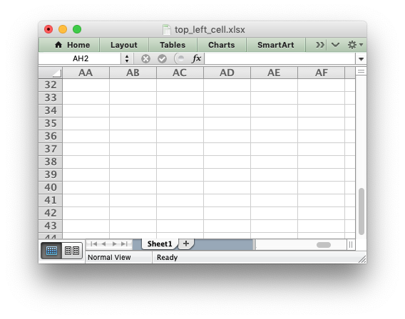
worksheet.set_top_left_cell()
Set the first visible cell at the top left of a worksheet.
| Parameters: |
|
|---|
This set_top_left_cell method can be used to set the top leftmost visible cell in the worksheet:
As shown above, both row-column and A1 style notation are supported. See Working with Cell Notation for more details.
worksheet.freeze_panes()
Create worksheet panes and mark them as frozen.
| Parameters: |
|
|---|
The freeze_panes() method can be used to divide a worksheet into horizontal or vertical regions known as panes and to “freeze” these panes so that the splitter bars are not visible.
The parameters row and col are used to specify the location of the split. It should be noted that the split is specified at the top or left of a cell and that the method uses zero based indexing. Therefore to freeze the first row of a worksheet it is necessary to specify the split at row 2 (which is 1 as the zero-based index).
You can set one of the row and col parameters as zero if you do not want either a vertical or horizontal split.
As shown above, both row-column and A1 style notation are supported. See Working with Cell Notation for more details.
The parameters top_row and left_col are optional. They are used to specify the top-most or left-most visible row or column in the scrolling region of the panes. For example to freeze the first row and to have the scrolling region begin at row twenty:
You cannot use A1 notation for the top_row and left_col parameters.
worksheet.split_panes()
Create worksheet panes and mark them as split.
| Parameters: |
|
|---|
The split_panes method can be used to divide a worksheet into horizontal or vertical regions known as panes. This method is different from the freeze_panes() method in that the splits between the panes will be visible to the user and each pane will have its own scroll bars.
The parameters y and x are used to specify the vertical and horizontal position of the split. The units for y and x are the same as those used by Excel to specify row height and column width. However, the vertical and horizontal units are different from each other. Therefore you must specify the y and x parameters in terms of the row heights and column widths that you have set or the default values which are 15 for a row and 8.43 for a column.
You can set one of the y and x parameters as zero if you do not want either a vertical or horizontal split. The parameters top_row and left_col are optional. They are used to specify the top-most or left-most visible row or column in the bottom-right pane.
You cannot use A1 notation with this method.
worksheet.set_zoom()
Set the worksheet zoom factor.
| Parameters: | zoom (int) – Worksheet zoom factor. |
|---|
Set the worksheet zoom factor in the range 10 zoom 400 :
The default zoom factor is 100. It isn’t possible to set the zoom to “Selection” because it is calculated by Excel at run-time.
Note, set_zoom() does not affect the scale of the printed page. For that you should use set_print_scale() .
worksheet.right_to_left()
Display the worksheet cells from right to left for some versions of Excel.
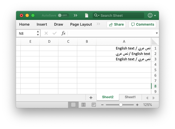
The right_to_left() method is used to change the default direction of the worksheet from left-to-right, with the A1 cell in the top left, to right-to-left, with the A1 cell in the top right:
This is useful when creating Arabic, Hebrew or other near or far eastern worksheets that use right-to-left as the default direction.
See also the Format set_reading_order() property to set the direction of the text within cells and the Example: Left to Right worksheets and text example program.
worksheet.hide_zero()
Hide zero values in worksheet cells.
The hide_zero() method is used to hide any zero values that appear in cells:
worksheet.set_background()
Set the background image for a worksheet.
| Parameters: |
|
|---|
The set_background() method can be used to set the background image for the worksheet:
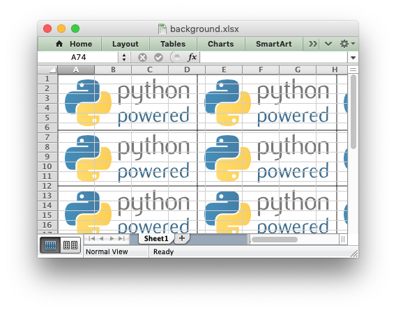
The set_background() method supports all the image formats supported by insert_image() .
Some people use this method to add a watermark background to their document. However, Microsoft recommends using a header image to set a watermark. The choice of method depends on whether you want the watermark to be visible in normal viewing mode or just when the file is printed. In XlsxWriter you can get the header watermark effect using set_header() :
It is also possible to pass an in-memory byte stream to set_background() if the is_byte_stream parameter is set to True. The stream should be io.BytesIO :
worksheet.set_tab_color()
Set the color of the worksheet tab.
| Parameters: | color (string) – The tab color. |
|---|
The set_tab_color() method is used to change the color of the worksheet tab:
The color can be a Html style #RRGGBB string or a limited number named colors, see Working with Colors .
worksheet.protect()
Protect elements of a worksheet from modification.
| Parameters: |
|
|---|
The protect() method is used to protect a worksheet from modification:
The protect() method also has the effect of enabling a cell’s locked and hidden properties if they have been set. A locked cell cannot be edited and this property is on by default for all cells. A hidden cell will display the results of a formula but not the formula itself. These properties can be set using the set_locked() and set_hidden() format methods.
You can optionally add a password to the worksheet protection:
The password should be an ASCII string. Passing the empty string » is the same as turning on protection without a password. See the note below on the “password” strength.
You can specify which worksheet elements you wish to protect by passing a dictionary in the options argument with any or all of the following keys:
The default boolean values are shown above. Individual elements can be protected as follows:
For chartsheets the allowable options and default values are:
Worksheet level passwords in Excel offer very weak protection. They do not encrypt your data and are very easy to deactivate. Full workbook encryption is not supported by XlsxWriter. However, it is possible to encrypt an XlsxWriter file using a third party open source tool called msoffice-crypt. This works for macOS, Linux and Windows:
worksheet.unprotect_range()
Unprotect ranges within a protected worksheet.
| Parameters: |
|
|---|
The unprotect_range() method is used to unprotect ranges in a protected worksheet. It can be used to set a single range or multiple ranges:
As in Excel the ranges are given sequential names like Range1 and Range2 but a user defined name can also be specified:
worksheet.set_default_row()
Set the default row properties.
| Parameters: |
|
|---|
The set_default_row() method is used to set the limited number of default row properties allowed by Excel which are the default height and the option to hide unused rows. These parameters are an optimization used by Excel to set row properties without generating a very large file with an entry for each row.
To set the default row height:
To hide unused rows:
worksheet.outline_settings()
Control outline settings.
| Parameters: |
|
|---|
The outline_settings() method is used to control the appearance of outlines in Excel. Outlines are described in Working with Outlines and Grouping :
The ‘visible’ parameter is used to control whether or not outlines are visible. Setting this parameter to False will cause all outlines on the worksheet to be hidden. They can be un-hidden in Excel by means of the “Show Outline Symbols” command button. The default setting is True for visible outlines.
The ‘symbols_below’ parameter is used to control whether the row outline symbol will appear above or below the outline level bar. The default setting is True for symbols to appear below the outline level bar.
The ‘symbols_right’ parameter is used to control whether the column outline symbol will appear to the left or the right of the outline level bar. The default setting is True for symbols to appear to the right of the outline level bar.
The ‘auto_style’ parameter is used to control whether the automatic outline generator in Excel uses automatic styles when creating an outline. This has no effect on a file generated by XlsxWriter but it does have an effect on how the worksheet behaves after it is created. The default setting is False for “Automatic Styles” to be turned off.
The default settings for all of these parameters correspond to Excel’s default parameters.
The worksheet parameters controlled by outline_settings() are rarely used.
worksheet.set_vba_name()
Set the VBA name for the worksheet.
| Parameters: | name (string) – The VBA name for the worksheet. |
|---|
The set_vba_name() method can be used to set the VBA codename for the worksheet (there is a similar method for the workbook VBA name). This is sometimes required when a vbaProject macro included via add_vba_project() refers to the worksheet. The default Excel VBA name of Sheet1 , etc., is used if a user defined name isn’t specified.
worksheet.ignore_errors()
Ignore various Excel errors/warnings in a worksheet for user defined ranges.
| Returns: | 0: Success. |
|---|---|
| Returns: | -1: Incorrect parameter or option. |
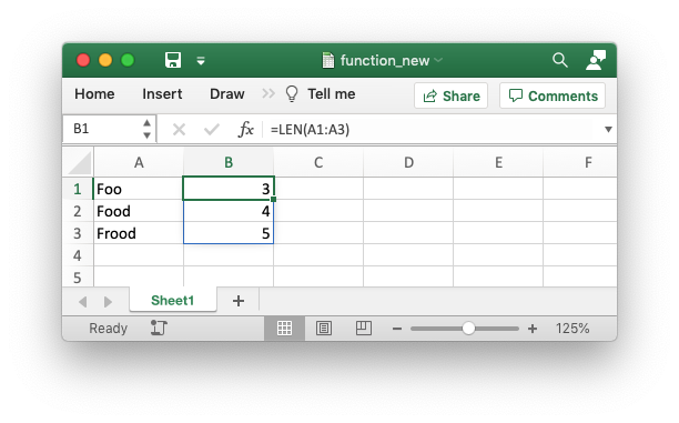
The ignore_errors() method can be used to ignore various worksheet cell errors/warnings. For example the following code writes a string that looks like a number:
This causes Excel to display a small green triangle in the top left hand corner of the cell to indicate an error/warning:
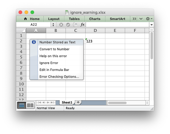
Sometimes these warnings are useful indicators that there is an issue in the spreadsheet but sometimes it is preferable to turn them off. Warnings can be turned off at the Excel level for all workbooks and worksheets by using the using “Excel options -> Formulas -> Error checking rules”. Alternatively you can turn them off for individual cells in a worksheet, or ranges of cells, using the ignore_errors() method with a dict of options and ranges like this:
The range can be a single cell, a range of cells, or multiple cells and ranges separated by spaces:
Note: calling ignore_errors() multiple times will overwrite the previous settings.
You can turn off warnings for an entire column by specifying the range from the first cell in the column to the last cell in the column:
Or for the entire worksheet by specifying the range from the first cell in the worksheet to the last cell in the worksheet:
The worksheet errors/warnings that can be ignored are:
- number_stored_as_text : Turn off errors/warnings for numbers stores as text.
- eval_error : Turn off errors/warnings for formula errors (such as divide by zero).
- formula_differs : Turn off errors/warnings for formulas that differ from surrounding formulas.
- formula_range : Turn off errors/warnings for formulas that omit cells in a range.
- formula_unlocked : Turn off errors/warnings for unlocked cells that contain formulas.
- empty_cell_reference : Turn off errors/warnings for formulas that refer to empty cells.
- list_data_validation : Turn off errors/warnings for cells in a table that do not comply with applicable data validation rules.
- calculated_column : Turn off errors/warnings for cell formulas that differ from the column formula.
- two_digit_text_year : Turn off errors/warnings for formulas that contain a two digit text representation of a year.
© Copyright 2013-2023, John McNamara.
Created using Sphinx 1.8.6.
Источник
In this article, we will discuss how to merge cells in an excel sheet using Python. We will use openpyxl module for merging cells.
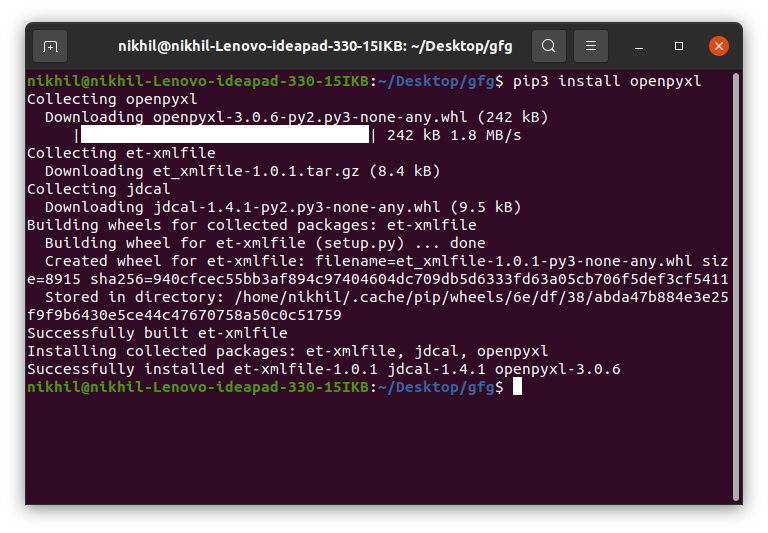
Installation of openpyxl using pip
pip install openpyxl
Implementation Of Merging Cells using openpyxl
Openpyxl provides a merge_cells() function for merging cells. When we merge cells, the top cell will be deleted from the worksheet. Openpyxl also provides an unmerged_cells() method for separating cells.
Syntax
merge_cells(range_string=None, start_row=None, start_column=None, end_row=None, end_column=None)
# import library
from openpyxl import Workbook
from openpyxl.styles import Alignment

work_book = Workbook()
work_sheet = work_book.active

# cells to merge
work_sheet.merge_cells('A1:D3')

cell = work_sheet.cell(row=1, column=1)
# value of cell
cell.value = 'quick fox jumps over the lazy dog'
# aligment of data in cell
cell.alignment = Alignment(horizontal='center', vertical='center')

# save the workbook
work_book.save('Excel_merge_cell.xlsx')
Also, refer
Find Column Number from Column Name in Excel using C++
Plot data from excel file in matplotlib Python
Write to an excel file using openpyxl module in Python
You all must have worked with Excel at some time in your life and must have felt the need for automating some repetitive or tedious task. Don’t worry in this tutorial we are going to learn about how to work with Excel using Python, or automating Excel using Python. We will be covering this with the help of the Openpyxl module.
Getting Started
Openpyxl is a Python library that provides various methods to interact with Excel Files using Python. It allows operations like reading, writing, arithmetic operations, plotting graphs, etc.
This module does not come in-built with Python. To install this type the below command in the terminal.
pip install openpyxl
Reading from Spreadsheets
To read an Excel file you have to open the spreadsheet using the load_workbook() method. After that, you can use the active to select the first sheet available and the cell attribute to select the cell by passing the row and column parameter. The value attribute prints the value of the particular cell. See the below example to get a better understanding.
Note: The first row or column integer is 1, not 0.
Dataset Used: It can be downloaded from here.
Example:
Python3
import openpyxl
path = "gfg.xlsx"
wb_obj = openpyxl.load_workbook(path)
sheet_obj = wb_obj.active
cell_obj = sheet_obj.cell(row = 1, column = 1)
print(cell_obj.value)
Output:
Name
Reading from Multiple Cells
There can be two ways of reading from multiple cells.
Method 1: We can get the count of the total rows and columns using the max_row and max_column respectively. We can use these values inside the for loop to get the value of the desired row or column or any cell depending upon the situation. Let’s see how to get the value of the first column and first row.
Example:
Python3
import openpyxl
path = "gfg.xlsx"
wb_obj = openpyxl.load_workbook(path)
sheet_obj = wb_obj.active
row = sheet_obj.max_row
column = sheet_obj.max_column
print("Total Rows:", row)
print("Total Columns:", column)
print("nValue of first column")
for i in range(1, row + 1):
cell_obj = sheet_obj.cell(row = i, column = 1)
print(cell_obj.value)
print("nValue of first row")
for i in range(1, column + 1):
cell_obj = sheet_obj.cell(row = 2, column = i)
print(cell_obj.value, end = " ")
Output:
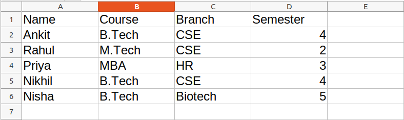
Total Rows: 6
Total Columns: 4

Value of first column
Name
Ankit
Rahul
Priya
Nikhil
Nisha

Value of first row
Ankit  B.Tech CSE 4
Method 2: We can also read from multiple cells using the cell name. This can be seen as the list slicing of Python.
Python3
import openpyxl
path = "gfg.xlsx"
wb_obj = openpyxl.load_workbook(path)
sheet_obj = wb_obj.active
cell_obj = sheet_obj['A1': 'B6']
for cell1, cell2 in cell_obj:
print(cell1.value, cell2.value)
Output:
Name Course
Ankit  B.Tech
Rahul M.Tech
Priya MBA
Nikhil B.Tech
Nisha B.Tech
Refer to the below article to get detailed information about reading excel files using openpyxl.
- Reading an excel file using Python openpyxl module
Writing to Spreadsheets
First, let’s create a new spreadsheet, and then we will write some data to the newly created file. An empty spreadsheet can be created using the Workbook() method. Let’s see the below example.
Example:
Python3
from openpyxl import Workbook
workbook = Workbook()
workbook.save(filename="sample.xlsx")
Output:
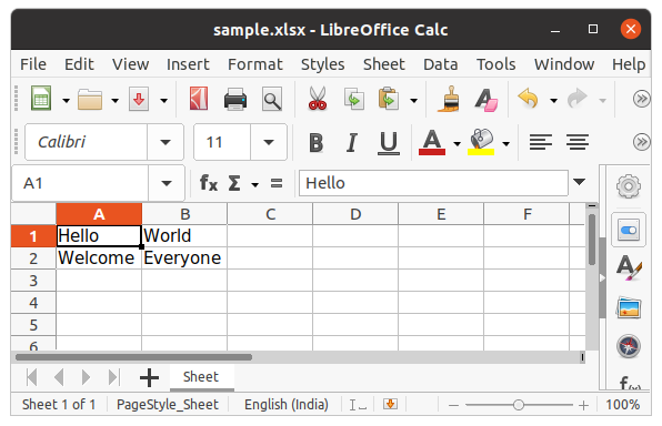
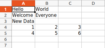
After creating an empty file, let’s see how to add some data to it using Python. To add data first we need to select the active sheet and then using the cell() method we can select any particular cell by passing the row and column number as its parameter. We can also write using cell names. See the below example for a better understanding.
Example:
Python3
import openpyxl
wb = openpyxl.Workbook()
sheet = wb.active
c1 = sheet.cell(row = 1, column = 1)
c1.value = "Hello"
c2 = sheet.cell(row= 1 , column = 2)
c2.value = "World"
c3 = sheet['A2']
c3.value = "Welcome"
c4 = sheet['B2']
c4.value = "Everyone"
wb.save("sample.xlsx")
Output:
Refer to the below article to get detailed information about writing to excel.
- Writing to an excel file using openpyxl module
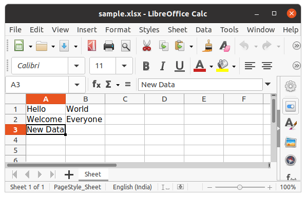
Appending to the Spreadsheet
In the above example, you will see that every time you try to write to a spreadsheet the existing data gets overwritten, and the file is saved as a new file. This happens because the Workbook() method always creates a new workbook file object. To write to an existing workbook you must open the file with the load_workbook() method. We will use the above-created workbook.
Example:
Python3
import openpyxl
wb = openpyxl.load_workbook("sample.xlsx")
sheet = wb.active
c = sheet['A3']
c.value = "New Data"
wb.save("sample.xlsx")
Output:
We can also use the append() method to append multiple data at the end of the sheet.
Example:
Python3
import openpyxl
wb = openpyxl.load_workbook("sample.xlsx")
sheet = wb.active
data = (
(1, 2, 3),
(4, 5, 6)
)
for row in data:
sheet.append(row)
wb.save('sample.xlsx')
Output:
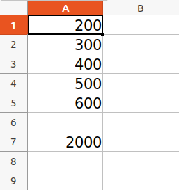
Arithmetic Operation on Spreadsheet
Arithmetic operations can be performed by typing the formula in a particular cell of the spreadsheet. For example, if we want to find the sum then =Sum() formula of the excel file is used.
Example:
Python3
import openpyxl
wb = openpyxl.Workbook()
sheet = wb.active
sheet['A1'] = 200
sheet['A2'] = 300
sheet['A3'] = 400
sheet['A4'] = 500
sheet['A5'] = 600
sheet['A7'] = '= SUM(A1:A5)'
wb.save("sum.xlsx")
Output:
Refer to the below article to get detailed information about the Arithmetic operations on Spreadsheet.
- Arithmetic operations in excel file using openpyxl
Adjusting Rows and Column
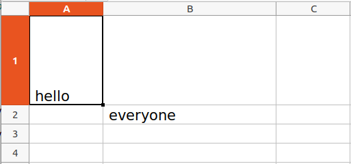
Worksheet objects have row_dimensions and column_dimensions attributes that control row heights and column widths. A sheet’s row_dimensions and column_dimensions are dictionary-like values; row_dimensions contains RowDimension objects and column_dimensions contains ColumnDimension objects. In row_dimensions, one can access one of the objects using the number of the row (in this case, 1 or 2). In column_dimensions, one can access one of the objects using the letter of the column (in this case, A or B).
Example:
Python3
import openpyxl
wb = openpyxl.Workbook()
sheet = wb.active
sheet.cell(row = 1, column = 1).value = ' hello '
sheet.cell(row = 2, column = 2).value = ' everyone '
sheet.row_dimensions[1].height = 70
sheet.column_dimensions['B'].width = 20
wb.save('sample.xlsx')
Output:
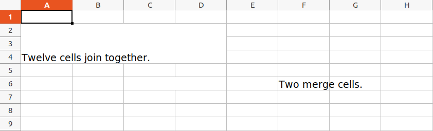
Merging Cells
A rectangular area of cells can be merged into a single cell with the merge_cells() sheet method. The argument to merge_cells() is a single string of the top-left and bottom-right cells of the rectangular area to be merged.
Example:
Python3
import openpyxl
wb = openpyxl.Workbook()
sheet = wb.active
sheet.merge_cells('A2:D4')
sheet.cell(row = 2, column = 1).value = 'Twelve cells join together.'
sheet.merge_cells('C6:D6')
sheet.cell(row = 6, column = 6).value = 'Two merge cells.'
wb.save('sample.xlsx')
Output:
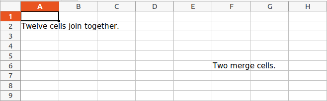
Unmerging Cells
To unmerge cells, call the unmerge_cells() sheet method.
Example:
Python3
import openpyxl
wb = openpyxl.load_workbook('sample.xlsx')
sheet = wb.active
sheet.unmerge_cells('A2:D4')
sheet.unmerge_cells('C6:D6')
wb.save('sample.xlsx')
Output:
Setting Font Style
To customize font styles in cells, important, import the Font() function from the openpyxl.styles module.
Example:
Python3
import openpyxl
from openpyxl.styles import Font
wb = openpyxl.Workbook()
sheet = wb.active
sheet.cell(row = 1, column = 1).value = "GeeksforGeeks"
sheet.cell(row = 1, column = 1).font = Font(size = 24 )
sheet.cell(row = 2, column = 2).value = "GeeksforGeeks"
sheet.cell(row = 2, column = 2).font = Font(size = 24, italic = True)
sheet.cell(row = 3, column = 3).value = "GeeksforGeeks"
sheet.cell(row = 3, column = 3).font = Font(size = 24, bold = True)
sheet.cell(row = 4, column = 4).value = "GeeksforGeeks"
sheet.cell(row = 4, column = 4).font = Font(size = 24, name = 'Times New Roman')
wb.save('sample.xlsx')
Output:
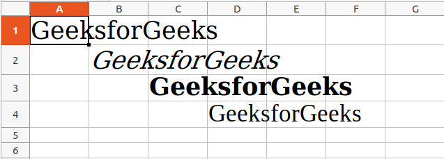
Refer to the below article to get detailed information about adjusting rows and columns.
- Adjusting rows and columns of an excel file using openpyxl module
Plotting Charts
Charts are composed of at least one series of one or more data points. Series themselves are comprised of references to cell ranges. For plotting the charts on an excel sheet, firstly, create chart objects of specific chart class( i.e BarChart, LineChart, etc.). After creating chart objects, insert data in it, and lastly, add that chart object in the sheet object.
Example 1:
Python3
import openpyxl
from openpyxl.chart import BarChart, Reference
wb = openpyxl.Workbook()
sheet = wb.active
for i in range(10):
sheet.append([i])
values = Reference(sheet, min_col=1, min_row=1,
max_col=1, max_row=10)
chart = BarChart()
chart.add_data(values)
chart.title = " BAR-CHART "
chart.x_axis.title = " X_AXIS "
chart.y_axis.title = " Y_AXIS "
sheet.add_chart(chart, "E2")
wb.save("sample.xlsx")
Output:
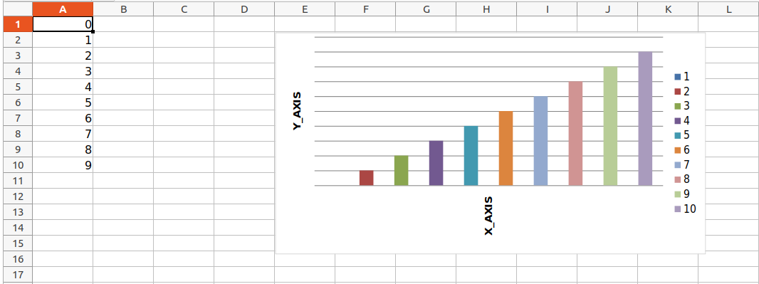
Example 2:
Python3
import openpyxl
from openpyxl.chart import LineChart, Reference
wb = openpyxl.Workbook()
sheet = wb.active
for i in range(10):
sheet.append([i])
values = Reference(sheet, min_col=1, min_row=1,
max_col=1, max_row=10)
chart = LineChart()
chart.add_data(values)
chart.title = " LINE-CHART "
chart.x_axis.title = " X-AXIS "
chart.y_axis.title = " Y-AXIS "
sheet.add_chart(chart, "E2")
wb.save("sample.xlsx")
Output:
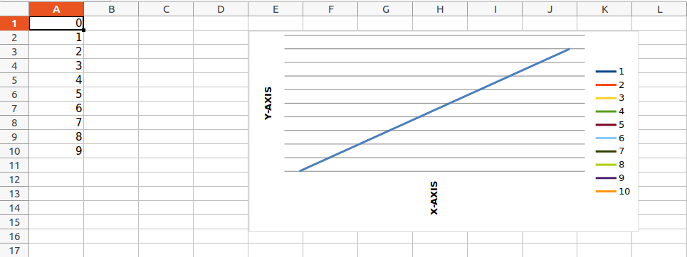
Refer to the below articles to get detailed information about plotting in excel using Python.
- Plotting charts in excel sheet using openpyxl module | Set 1
- Plotting charts in excel sheet using openpyxl module | Set 2
- Plotting charts in excel sheet using openpyxl module | Set 3
Adding Images
For the purpose of importing images inside our worksheet, we would be using openpyxl.drawing.image.Image. The method is a wrapper over PIL.Image method found in PIL (pillow) library. Due to which it is necessary for the PIL (pillow) library to be installed in order to use this method.
Image Used:

Example:
Python3
import openpyxl
from openpyxl.drawing.image import Image
wb = openpyxl.Workbook()
sheet = wb.active
sheet.append([10, 2010, "Geeks", 4, "life"])
img = Image("geek.jpg")
sheet.add_image(img, 'A2')
wb.save('sample.xlsx')
Output:
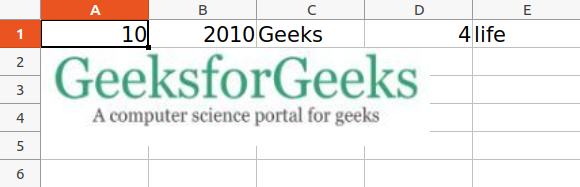
Refer to the below article to get detailed information about adding images.
- Openpyxl – Adding Image
Some More Functionality of Excel using Python
- How to delete one or more rows in excel using Openpyxl?
- Trigonometric operations in excel file using openpyxl
- How to copy data from one excel sheet to another
- How to Automate an Excel Sheet in Python?
Skip to content
![]()
In this tutorial, we will learn how to merge/unmerge cells in an excel file and assign the value to unmerged cells in an excel sheet using the openpyxl module in python. In openpyxl, we will use the merge_cells() built-in function to merge cells and unmerge_cells() to unmerge the cells.Before jumping into the coding section download the sample excel file by clicking the download sample file button or you can use your document as well.
Below is the snapshot of the input sheet.We are going to merge red outlined cells.

Source Code:
import openpyxl
from openpyxl.styles import Alignment
wbook=openpyxl.load_workbook("openpyxl_merge_unmerge.xlsx")
sheet=wbook["merge_sample"]
data=sheet['B4'].value
sheet.merge_cells('B4:E4')
sheet['B4']=data
sheet['B4'].alignment = Alignment(horizontal='center')
wbook.save("openpyxl_merge_unmerge.xlsx")
exit()
Now save the above program and give a name merge_openpyxl.py then execute the file as shown below.![]()
Output:

Unmerge:
Below is the snapshot of the excel sheet on which we are going to perform an unmerged operation. Also, we will assign the value to unmerged cells as well.
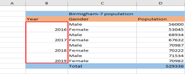
Source code:
import openpyxl
from openpyxl.utils import range_boundaries
wbook=openpyxl.load_workbook("openpyxl_merge_unmerge.xlsx")
sheet=wbook["unmerge_sample"]
for cell_group in sheet.merged_cells.ranges:
	min_col, min_row, max_col, max_row = range_boundaries(str(cell_group))
	top_left_cell_value = sheet.cell(row=min_row, column=min_col).value
	sheet.unmerge_cells(str(cell_group))
	for row in sheet.iter_rows(min_col=min_col, min_row=min_row, max_col=max_col, max_row=max_row):
		for cell in row:
			cell.value = top_left_cell_value
wbook.save("openpyxl_merge_unmerge.xlsx")
exit()
Now save the above program and give a name unmerge_openpyxl.py and execute the program as shown below.

Output:

Документ электронной таблицы Excel называется рабочей книгой. Каждая книга может хранить некоторое количество листов. Лист, просматриваемый пользователем в данный момент, называется активным. Лист состоит из из столбцов (адресуемых с помощью букв, начиная с A) и строк (адресуемых с помощью цифр, начиная с 1).
Модуль OpenPyXL не поставляется вместе с Python, поэтому его предварительно нужно установить:
> pip install openpyxl
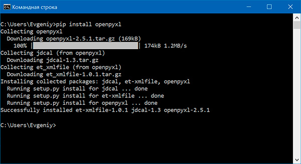
Чтение файлов Excel
Начинаем работать:
>>> import openpyxl
>>> wb = openpyxl.load_workbook('example.xlsx')
>>> type(wb)
<class 'openpyxl.workbook.workbook.Workbook'>
>>> wb.sheetnames
['Лист1', 'Лист2', 'Лист3']
>>> sheet = wb.active
>>> sheet
<Worksheet "Лист1">
>>> sheet['A1']
<Cell Лист1.A1>
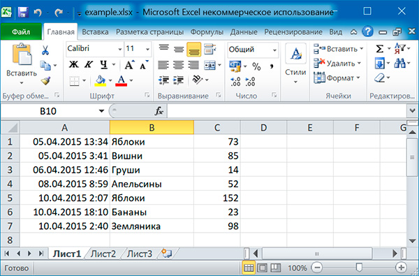
А теперь небольшой скрипт:
import openpyxl

# читаем excel-файл
wb = openpyxl.load_workbook('example.xlsx')

# печатаем список листов
sheets = wb.sheetnames
for sheet in sheets:
    print(sheet)

# получаем активный лист
sheet = wb.active

# печатаем значение ячейки A1
print(sheet['A1'].value)
# печатаем значение ячейки B1
print(sheet['B1'].value)
Результат работы:
Лист1
Лист2
Лист3

2015-04-05 13:34:02
Яблоки
Как получить другой лист книги:
# получаем другой лист
sheet2 = wb['Лист2']
# печатаем значение ячейки A1
print(sheet2['A2'].value)
Как сделать лист книги активным:
# делаем третий лист активным
wb.active = 2
Как задать имя листа:
sheet.title = 'Третий лист'
Объект Cell имеет атрибут value, который содержит значение, хранящееся в ячейке. Объект Cell также имеет атрибуты row, column и coordinate, которые предоставляют информацию о расположении данной ячейки в таблице.
# получаем ячейку листа B2
cell = sheet['B2']
print('Строка: ' + str(cell.row))
print('Столбец: ' + cell.column)
print('Ячейка: ' + cell.coordinate)
print('Значение: ' + cell.value)
Строка: 2
Столбец: B
Ячейка: B2
Значение: Вишни
К отдельной ячейке можно также обращаться с помощью метода cell() объекта Worksheet, передавая ему именованные аргументы row и column. Первому столбцу или первой строке соответствует число 1, а не 0:
# получаем ячейку листа B2
cell = sheet.cell(row = 2, column = 2)
print(cell.value)
Вишни
Размер листа можно получить с помощью атрибутов max_row и max_column объекта Worksheet:
rows = sheet.max_row
cols = sheet.max_column

for i in range(1, rows + 1):
    string = ''
    for j in range(1, cols + 1):
        cell = sheet.cell(row = i, column = j)
        string = string + str(cell.value) + ' '
    print(string)
2015-04-05 13:34:02 Яблоки 73
2015-04-05 03:41:23 Вишни 85
2015-04-06 12:46:51 Груши 14
2015-04-08 08:59:43 Апельсины 52
2015-04-10 02:07:00 Яблоки 152
2015-04-10 18:10:37 Бананы 23
2015-04-10 02:40:46 Земляника 98
Чтобы преобразовать буквенное обозначение столбца в цифровое, следует вызвать функцию
openpyxl.utils.column_index_from_string()
Чтобы преобразовать цифровое обозначение столбуа в буквенное, следует вызвать функцию
openpyxl.utils.get_column_letter()
Для вызова этих функций загружать рабочую книгу не обязательно.
>>> from openpyxl.utils import get_column_letter, column_index_from_string
>>> get_column_letter(1)
'A'
>>> get_column_letter(27)
'AA'
>>> column_index_from_string('A')
1
>>> column_index_from_string('AA')
27
Используя срезы объектов Worksheet, можно получить все объекты Cell, принадлежащие определенной строке, столбцу или прямоугольной области.
>>> sheet['A1':'C3']
((<Cell 'Лист1'.A1>, <Cell 'Лист1'.B1>, <Cell 'Лист1'.C1>),
 (<Cell 'Лист1'.A2>, <Cell 'Лист1'.B2>, <Cell 'Лист1'.C2>),
 (<Cell 'Лист1'.A3>, <Cell 'Лист1'.B3>, <Cell 'Лист1'.C3>))
for row in sheet['A1':'C3']:
    string = ''
    for cell in row:
        string = string + str(cell.value) + ' '
    print(string)
2015-04-05 13:34:02 Яблоки 73
2015-04-05 03:41:23 Вишни 85
2015-04-06 12:46:51 Груши 14
Выводим значения второй колонки:
>>> sheet['B']
(<Cell 'Лист1'.B1>, <Cell 'Лист1'.B2>, <Cell 'Лист1'.B3>, <Cell 'Лист1'.B4>, ..., <Cell 'Лист1'.B7>)
for cell in sheet['B']:
    print(cell.value)
Яблоки
Вишни
Груши
Апельсины
Яблоки
Бананы
Земляника
Выводим строки с первой по третью:
>>> sheet[1:3]
((<Cell 'Лист1'.A1>, <Cell 'Лист1'.B1>, <Cell 'Лист1'.C1>),
 (<Cell 'Лист1'.A2>, <Cell 'Лист1'.B2>, <Cell 'Лист1'.C2>),
 (<Cell 'Лист1'.A3>, <Cell 'Лист1'.B3>, <Cell 'Лист1'.C3>))
for row in sheet[1:3]:
    string = ''
    for cell in row:
        string = string + str(cell.value) + ' '
    print(string)
2015-04-05 13:34:02 Яблоки 73
2015-04-05 03:41:23 Вишни 85
2015-04-06 12:46:51 Груши 14
Для доступа к ячейкам конкретной строки или столбца также можно воспользоваться атрибутами rows и columns объекта Worksheet.
>>> list(sheet.rows)
[(<Cell 'Лист1'.A1>, <Cell 'Лист1'.B1>, <Cell 'Лист1'.C1>),
 (<Cell 'Лист1'.A2>, <Cell 'Лист1'.B2>, <Cell 'Лист1'.C2>),
 ..........
 (<Cell 'Лист1'.A6>, <Cell 'Лист1'.B6>, <Cell 'Лист1'.C6>),
 (<Cell 'Лист1'.A7>, <Cell 'Лист1'.B7>, <Cell 'Лист1'.C7>)]
for row in sheet.rows:
    print(row)
(<Cell 'Лист1'.A1>, <Cell 'Лист1'.B1>, <Cell 'Лист1'.C1>)
(<Cell 'Лист1'.A2>, <Cell 'Лист1'.B2>, <Cell 'Лист1'.C2>)
..........
(<Cell 'Лист1'.A6>, <Cell 'Лист1'.B6>, <Cell 'Лист1'.C6>)
(<Cell 'Лист1'.A7>, <Cell 'Лист1'.B7>, <Cell 'Лист1'.C7>)
>>> list(sheet.columns)
[(<Cell 'Лист1'.A1>, <Cell 'Лист1'.A2>, <Cell 'Лист1'.A3>, <Cell 'Лист1'.A4>, ..., <Cell 'Лист1'.A7>),
 (<Cell 'Лист1'.B1>, <Cell 'Лист1'.B2>, <Cell 'Лист1'.B3>, <Cell 'Лист1'.B4>, ..., <Cell 'Лист1'.B7>),
 (<Cell 'Лист1'.C1>, <Cell 'Лист1'.C2>, <Cell 'Лист1'.C3>, <Cell 'Лист1'.C4>, ..., <Cell 'Лист1'.C7>)]
for column in sheet.columns:
    print(column)
(<Cell 'Лист1'.A1>, <Cell 'Лист1'.A2>, <Cell 'Лист1'.A3>, <Cell 'Лист1'.A4>, ..., <Cell 'Лист1'.A7>)
(<Cell 'Лист1'.B1>, <Cell 'Лист1'.B2>, <Cell 'Лист1'.B3>, <Cell 'Лист1'.B4>, ..., <Cell 'Лист1'.B7>)
(<Cell 'Лист1'.C1>, <Cell 'Лист1'.C2>, <Cell 'Лист1'.C3>, <Cell 'Лист1'.C4>, ..., <Cell 'Лист1'.C7>)
Выводим значения всех ячеек листа:
for row in sheet.rows:
    string = ''
    for cell in row:
        string = string + str(cell.value) + ' '
    print(string)
2015-04-05 13:34:02 Яблоки 73
2015-04-05 03:41:23 Вишни 85
2015-04-06 12:46:51 Груши 14
2015-04-08 08:59:43 Апельсины 52
2015-04-10 02:07:00 Яблоки 152
2015-04-10 18:10:37 Бананы 23
2015-04-10 02:40:46 Земляника 98
Выводим значения второй строки (индекс 1):
for cell in list(sheet.rows)[1]:
    print(str(cell.value))
2015-04-05 03:41:23
Вишни
85
Выводим значения второй колонки (индекс 1):
for row in sheet.rows:
    print(str(row[1].value))
Яблоки
Вишни
Груши
Апельсины
Яблоки
Бананы
Земляника
Запись файлов Excel
>>> import openpyxl
>>> wb = openpyxl.Workbook()
>>> wb.sheetnames
['Sheet']
>>> wb.create_sheet(title = 'Первый лист', index = 0)
<Worksheet "Первый лист">
>>> wb.sheetnames
['Первый лист', 'Sheet']
>>> wb.remove(wb['Первый лист'])
>>> wb.sheetnames
['Sheet']
>>> wb.save('example.xlsx')
Метод create_sheet() возвращает новый объект Worksheet, который по умолчанию становится последним листом книги. С помощью именованных аргументов title и index можно задать имя и индекс нового листа.
Метод remove() принимает в качестве аргумента не строку с именем листа, а объект Worksheet. Если известно только имя листа, который надо удалить, используйте wb[sheetname]. Еще один способ удалить лист — использовать инструкцию del wb[sheetname].
Не забудьте вызвать метод save(), чтобы сохранить изменения после добавления или удаления листа рабочей книги.
Запись значений в ячейки напоминает запись значений в ключи словаря:
>>> import openpyxl
>>> wb = openpyxl.Workbook()
>>> wb.create_sheet(title = 'Первый лист', index = 0)
>>> sheet = wb['Первый лист']
>>> sheet['A1'] = 'Здравствуй, мир!'
>>> sheet['A1'].value
'Здравствуй, мир!'
Заполняем таблицу 3×3:
import openpyxl

# создаем новый excel-файл
wb = openpyxl.Workbook()

# добавляем новый лист
wb.create_sheet(title = 'Первый лист', index = 0)

# получаем лист, с которым будем работать
sheet = wb['Первый лист']

for row in range(1, 4):
    for col in range(1, 4):
        value = str(row) + str(col)
        cell = sheet.cell(row = row, column = col)
        cell.value = value

wb.save('example.xlsx')
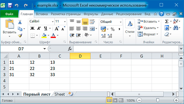
Можно добавлять строки целиком:
sheet.append(['Первый', 'Второй', 'Третий'])
sheet.append(['Четвертый', 'Пятый', 'Шестой'])
sheet.append(['Седьмой', 'Восьмой', 'Девятый'])
Стилевое оформление
Для настройки шрифтов, используемых в ячейках, необходимо импортировать функцию Font() из модуля openpyxl.styles:
from openpyxl.styles import Font
Ниже приведен пример создания новой рабочей книги, в которой для шрифта, используемого в ячейке A1, устанавливается шрифт Arial, красный цвет, курсивное начертание и размер 24 пункта:
import openpyxl
from openpyxl.styles import Font

# создаем новый excel-файл
wb = openpyxl.Workbook()
# добавляем новый лист
wb.create_sheet(title = 'Первый лист', index = 0)
# получаем лист, с которым будем работать
sheet = wb['Первый лист']

font = Font(name='Arial', size=24, italic=True, color='FF0000')
sheet['A1'].font = font
sheet['A1'] = 'Здравствуй мир!'

# записываем файл
wb.save('example.xlsx')
Именованные стили применяются, когда надо применить стилевое оформление к большому количеству ячеек.
import openpyxl
from openpyxl.styles import NamedStyle, Font, Border, Side

# создаем новый excel-файл
wb = openpyxl.Workbook()
# добавляем новый лист
wb.create_sheet(title = 'Первый лист', index = 0)
# получаем лист, с которым будем работать
sheet = wb['Первый лист']

# создаем именованный стиль
ns = NamedStyle(name='highlight')
ns.font = Font(bold=True, size=20)
border = Side(style='thick', color='000000')
ns.border = Border(left=border, top=border, right=border, bottom=border)

# вновь созданный именованный стиль надо зарегистрировать
# для дальнейшего использования
wb.add_named_style(ns)

# теперь можно использовать именованный стиль
sheet['A1'].style = 'highlight'

# записываем файл
wb.save('example.xlsx')
Добавление формул
Формулы, начинающиеся со знака равенства, позволяют устанавливать для ячеек значения, рассчитанные на основе значений в других ячейках.
sheet['B9'] = '=SUM(B1:B8)'
Эта инструкция сохранит =SUM(B1:B8) в качестве значения в ячейке B9. Тем самым для ячейки B9 задается формула, которая суммирует значения, хранящиеся в ячейках от B1 до B8.
Формула Excel — это математическое выражение, которое создается для вычисления результата и которое может зависеть от содержимого других ячеек. Формула в ячейке Excel может содержать данные, ссылки на другие ячейки, а также обозначение действий, которые необходимо выполнить.
Использование ссылок на ячейки позволяет пересчитывать результат по формулам, когда происходят изменения содержимого ячеек, включенных в формулы. Формулы Excel начинаются со знака =. Скобки () могут использоваться для определения порядка математических операции.
Примеры формул Excel: =27+36, =А1+А2-АЗ, =SUM(А1:А5), =MAX(АЗ:А5), =(А1+А2)/АЗ.
Хранящуюся в ячейке формулу можно читать, как любое другое значение. Однако, если нужно получить результат расчета по формуле, а не саму формулу, то при вызове функции load_workbook() ей следует передать именованный аргумент data_only со значением True.
Настройка строк и столбцов
С помощью модуля OpenPyXL можно задавать высоту строк и ширину столбцов таблицы, закреплять их на месте (чтобы они всегда были видны на экране), полностью скрывать из виду, объединять ячейки.
Настройка высоты строк и ширины столбцов
Объекты Worksheet имеют атрибуты row_dimensions и column_dimensions, которые управляют высотой строк и шириной столбцов.
sheet['A1'] = 'Высокая строка'
sheet['B2'] = 'Широкий столбец'

sheet.row_dimensions[1].height = 70
sheet.column_dimensions['B'].width = 30
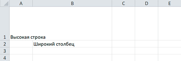
Атрибуты row_dimensions и column_dimensions представляют собой значения, подобные словарю. Атрибут row_dimensions содержит объекты RowDimensions, а атрибут column_dimensions содержит объекты ColumnDimensions. Доступ к объектам в row_dimensions осуществляется с использованием номера строки, а доступ к объектам в column_dimensions — с использованием буквы столбца.
Для указания высоты строки разрешено использовать целые или вещественные числа в диапазоне от 0 до 409. Для указания ширины столбца можно использовать целые или вещественные числа в диапазоне от 0 до 255. Столбцы с нулевой шириной и строки с нулевой высотой невидимы для пользователя.
Объединение ячеек
Ячейки, занимающие прямоугольную область, могут быть объединены в одну ячейку с помощью метода merge_cells() рабочего листа:
sheet.merge_cells('A1:D3')
sheet['A1'] = 'Объединены двенадцать ячеек'

sheet.merge_cells('C5:E5')
sheet['C5'] = 'Объединены три ячейки'
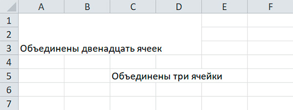
Чтобы отменить слияние ячеек, надо вызвать метод unmerge_cells():
sheet.unmerge_cells('A1:D3')
sheet.unmerge_cells('C5:E5')
Закрепление областей
Если размер таблицы настолько велик, что ее нельзя увидеть целиком, можно заблокировать несколько верхних строк или крайних слева столбцов в их позициях на экране. В этом случае пользователь всегда будет видеть заблокированные заголовки столбцов или строк, даже если он прокручивает таблицу на экране.
У объекта Worksheet имеется атрибут freeze_panes, значением которого может служить объект Cell или строка с координатами ячеек. Все строки и столбцы, расположенные выше и левее, будут заблокированы.
| Значение атрибута freeze_panes | Заблокированные строки и столбцы |
|---|---|
sheet.freeze_panes = 'A2' |
Строка 1 |
sheet.freeze_panes = 'B1' |
Столбец A |
sheet.freeze_panes = 'C1' |
Столбцы A и B |
sheet.freeze_panes = 'C2' |
Строка 1 и столбцы A и B |
sheet.freeze_panes = None |
Закрепленные области отсутствуют |
Диаграммы
Модуль OpenPyXL поддерживает создание гистогорамм, графиков, а также точечных и круговых диаграмм с использование данных, хранящихся в электронной таблице. Чтобы создать диаграмму, необходимо выполнить следующие действия:
- создать объект
Referenceна основе ячеек в пределах выделенной прямоугольной области; - создать объект
Series, передав функцииSeries()объектReference; - создать объект Chart;
- дополнительно можно установить значения переменных
drawing.top,drawing.left,drawing.width,drawing.heightобъектаChart, определяющих положение и размеры диаграммы; - добавить объект
Chartв объектWorksheet.
Объекты Reference создаются путем вызова функции openpyxl.charts.Reference(), принимающей пять аргуменов:
- Объект
Worksheet, содержащий данные диаграммы. - Два целых числа, представляющих верхнюю левую ячейку выделенной прямоугольной области, в которых содержатся данные диаграммы: первое число задает строку, второе — столбец; первой строке соответствует 1, а не 0.
- Два целых числа, представляющих нижнюю правую ячейку выделенной прямоугольной области, в которых содержатся данные диаграммы: первое число задает строку, второе — столбец.
from openpyxl import Workbook
from openpyxl.chart import BarChart, Reference

# создаем новый excel-файл
wb = Workbook()
# добавляем новый лист
wb.create_sheet(title = 'Первый лист', index = 0)
# получаем лист, с которым будем работать
sheet = wb['Первый лист']

sheet['A1'] = 'Серия 1'
# это колонка с данными
for i in range(1, 11):
    cell = sheet.cell(row = i + 1, column = 1)
    cell.value = i * i

# создаем диаграмму
chart = BarChart()
chart.title = 'Первая серия данных'
data = Reference(sheet, min_col = 1, min_row = 1, max_col = 1, max_row = 11)
chart.add_data(data, titles_from_data = True)

# добавляем диаграмму на лист
sheet.add_chart(chart, 'C2')

# записываем файл
wb.save('example.xlsx')
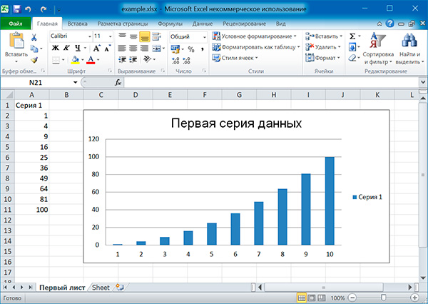
Аналогично можно создавать графики, точечные и круговые диаграммы, вызывая методы:
openpyxl.chart.LineChart()openpyxl.chart.ScatterChart()openpyxl.chart.PieChart()
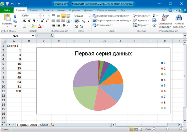
Поиск:
Excel • MS • Python • Web-разработка • Модуль
Reading Excel spreadsheets is all well and good. However, you also need to be able to create or edit a spreadsheet. The focus of this chapter will be on learning how to do that! OpenPyXL lets you create Microsoft Excel spreadsheets with a minimum of fuss.
Creating Excel spreadsheets using Python allows you to generate a new type of report that your users will use. For example, you might receive your data from a client in the form of JSON or XML. These data formats are not something that most accountants or business people are used to reading.
Once you learn how to create Excel spreadsheets with Python, you can leverage that knowledge to transform other data into Excel spreadsheets. This knowledge also allows you to do the reverse, taking in an Excel spreadsheet and output a different format, such as JSON or XML.
In this article, you will learn how to use OpenPyXL to do the following:
- Create a spreadsheet
- Write to a spreadsheet
- Add and remove sheets
- Insert and delete rows and columns
- Edit cell data
- Create merged cells
- Fold rows and columns
Let’s get started by creating a brand new spreadsheet!
Editor’s note: This article is based on a chapter from the book: Automating Excel with Python. You can order a copy on Gumroad or Kickstarter.
Creating a Spreadsheet
Creating an empty spreadsheet using OpenPyXL doesn’t take much code. Open up your Python editor and create a new file. Name it creating_spreadsheet.py.
Now add the following code to your file:
# creating_spreadsheet.py

from openpyxl import Workbook


def create_workbook(path):
    workbook = Workbook()
    workbook.save(path)


if __name__ == "__main__":
    create_workbook("hello.xlsx")
The critical piece here is that you need to import the Workbook class. This class allows you to instantiate a workbook object that you can then save. All this code does is create the file that you pass to it and save it.
Your new spreadsheet will look like this:
Now you’re ready to learn how to add some data to the cells in your spreadsheet.
Writing to a Spreadsheet
When writing data in a spreadsheet, you need to get the “sheet” object. You learned how to do that in the previous chapter using workbook.active, which gives you the active or currently visible sheet. You could also explicitly tell OpenPyXL which sheet you want to access by passing it a sheet title.
For this example, you will create another new program and then use the active sheet. Open up a new file and name it adding_data.py. Now add this code to your file:
# adding_data.py

from openpyxl import Workbook


def create_workbook(path):
    workbook = Workbook()
    sheet = workbook.active
    sheet["A1"] = "Hello"
    sheet["A2"] = "from"
    sheet["A3"] = "OpenPyXL"
    workbook.save(path)


if __name__ == "__main__":
    create_workbook("hello.xlsx")
This code will overwrite the previous example’s Excel spreadsheet. After you create the Workbook() object, you grab the active Worksheet. Then you add text strings to the cells: A1, A2, and A3. The last step is to save your new spreadsheet.
When you run this code, your new spreadsheet will look like this:
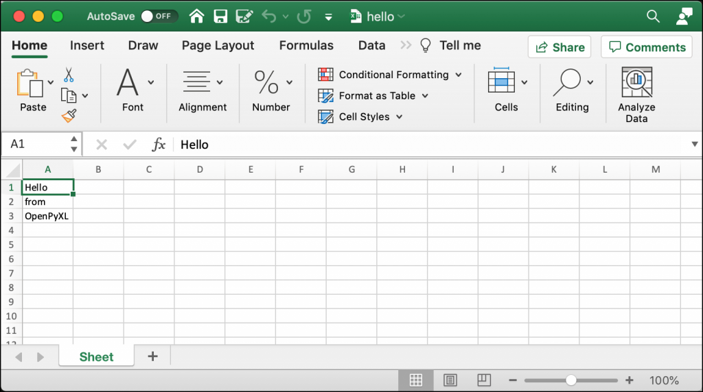
You can use this technique to write data to any cell in your spreadsheet.
Now let’s find out how to add and remove a worksheet!
Adding and Removing Sheets
Adding a worksheet to a workbook happens automatically when you create a new Workbook. The Worksheet will be named “Sheet” by default. If you want, you can set the name of the sheet yourself.
To see how this works, create a new file named creating_sheet_title.py and add the following code:
# creating_sheet_title.py

from openpyxl import Workbook


def create_sheets(path):
    workbook = Workbook()
    sheet = workbook.active
    sheet.title = "Hello"
    sheet2 = workbook.create_sheet(title="World")
    workbook.save(path)


if __name__ == "__main__":
    create_sheets("hello_sheets.xlsx")
Here you create the Workbook and then grab the active Worksheet. You can then set the Worksheet’s title using the title attribute. The following line of code adds a new worksheet to the Workbook by calling create_sheet().
The create_sheet() method takes two parameters: title and index. The title attribute gives a title to the Worksheet. The index tells the Workbook where to insert the Worksheet, from left to right. If you specify zero, your Worksheet gets inserted at the beginning.
If you run this code, your new spreadsheet will look like this:
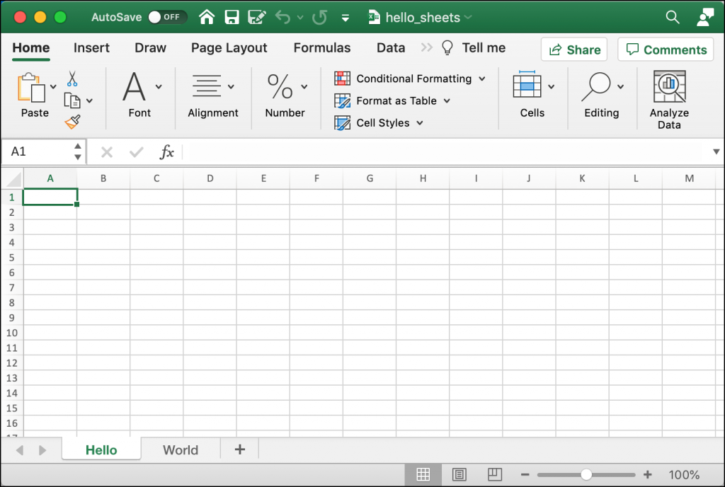
Sometimes you will need to delete a worksheet. Perhaps that sheet no longer has valid information, or it was created by accident.
To see how to delete a worksheet, create another new file and name it delete_sheets.py. Then add this code:
# delete_sheets.py

import openpyxl


def create_worksheets(path):
    workbook = openpyxl.Workbook()
    workbook.create_sheet()
    print(workbook.sheetnames)
    # Insert a worksheet
    workbook.create_sheet(index=1, title="Second sheet")
    print(workbook.sheetnames)
    del workbook["Second sheet"]
    print(workbook.sheetnames)
    workbook.save(path)


if __name__ == "__main__":
    create_worksheets("del_sheets.xlsx")
In this example, you create two new sheets. The first Worksheet has no title specified, so it defaults to “Sheet1”. You supply a title to the second sheet, and then you print out all the current worksheet titles.
Next, you use Python’s del keyword to delete the Worksheet’s name from the workbook, which removes the sheet. Then you print out the current worksheet titles again.
Here is the output from running the code:
['Sheet', 'Sheet1']
['Sheet', 'Second sheet', 'Sheet1']
['Sheet', 'Sheet1']
The first Worksheet gets created automatically when you instantiate the Workbook. The Worksheet is named “Sheet”. Then you make “Sheet1”. Lastly, you create “Second sheet”, but you insert it at position 1, which tells the Workbook to shift ‘Sheet1’ to the right by one position.
You can see from the output above how the worksheets are ordered before and after you add and delete the “Second sheet”.
Now let’s learn about inserting and removing rows and columns!
Inserting and Deleting Rows and Columns
The OpenPyXL package provides you with several methods that you can use to insert or delete rows and columns. These methods are a part of the Worksheet object.
You will learn about the following four methods:
.insert_rows().delete_rows().insert_cols().delete_cols()
Each of these methods can take these two arguments:
idx– The index to insert into (or delete from)amount– The number of rows or columns to add (or delete)
You can use the insert methods to insert rows or columns at the specified index.
Open up a new file and name it insert_demo.py. Then enter this code in your new file:
# insert_demo.py

from openpyxl import Workbook


def inserting_cols_rows(path):
    workbook = Workbook()
    sheet = workbook.active
    sheet["A1"] = "Hello"
    sheet["A2"] = "from"
    sheet["A3"] = "OpenPyXL"
    # insert a column before A
    sheet.insert_cols(idx=1)
    # insert 2 rows starting on the second row
    sheet.insert_rows(idx=2, amount=2)
    workbook.save(path)


if __name__ == "__main__":
    inserting_cols_rows("inserting.xlsx")
Here you create another new Spreadsheet. In this case, you add text to the first three cells in the “A” column. Then you insert one column at index one. That means you inserted a single column before “A”, which causes the cells in column “A” to shift to column “B”.
Next, you insert two new rows starting at index two. This code will insert two rows between the first and second rows.
You can see how this changes things by taking a look at the following screenshot:
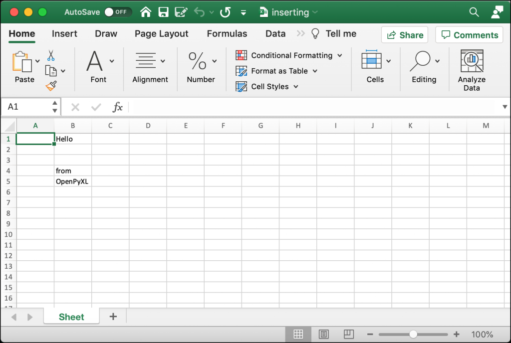
Try changing the indexes or number of rows and columns that you want to insert and see how it works.
You will also need to delete columns and rows from time to time. To do that you will use .delete_rows() and .delete_cols().
Open up a new file and name it delete_demo.py. Then add this code:
# delete_demo.py

from openpyxl import Workbook


def deleting_cols_rows(path):
    workbook = Workbook()
    sheet = workbook.active
    sheet["A1"] = "Hello"
    sheet["B1"] = "from"
    sheet["C1"] = "OpenPyXL"
    sheet["A2"] = "row 2"
    sheet["A3"] = "row 3"
    sheet["A4"] = "row 4"
    # Delete column A
    sheet.delete_cols(idx=1)
    # delete 2 rows starting on the second row
    sheet.delete_rows(idx=2, amount=2)
    workbook.save(path)


if __name__ == "__main__":
    deleting_cols_rows("deleting.xlsx")
In this example, you add text to six different cells. Four of those cells are in column “A”. Then you use delete_cols() to delete column “A”! That means you got rid of four values. Next, you delete two rows, starting at row number two.
When you run this code, your result should look like this:
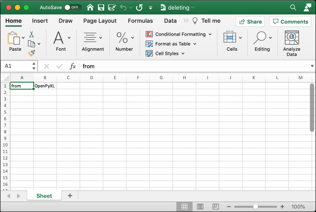
Try editing the index or amount values to get familiar with deleting rows and columns.
Now you are ready to learn about editing a spreadsheet’s values!
Editing Cell Data
You can use OpenPyXL to change the values in a pre-existing Excel spreadsheet. You can do that by specifying the cell you want to change and then setting it to a new value.
For this example, you will use the inserting.xlsx file you created in the previous section. Now create a new Python file named editing_demo.py. Then add the following code:
# editing_demo.py

from openpyxl import load_workbook


def edit(path, data):
    workbook = load_workbook(filename=path)
    sheet = workbook.active
    for cell in data:
        current_value = sheet[cell].value
        sheet[cell] = data[cell]
        print(f'Changing {cell} from {current_value} to {data[cell]}')
    workbook.save(path)

if __name__ == "__main__":
    data = {"B1": "Hi", "B5": "Python"}
    edit("inserting.xlsx", data)
This code loads up the Excel file that you created in the previous section. It then loops over each value in the data dictionary that you passed to the edit() function. You get the current value for the cell using a key in the dictionary. Then you change that cell’s value to match the value in the dictionary.
To make it more obvious what is going on, you print out the old and new values of the cell.
When you run this code, you will see the following output:
Changing B1 from Hello to Hi
Changing B5 from OpenPyXL to Python
Open up the new version of the inserting.xlsx file, and it should now look like this:
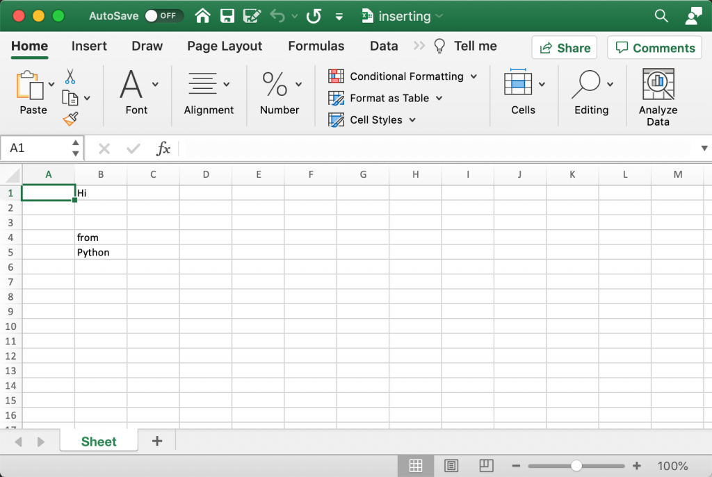
Here you can see how the cell values have changed to match the one specified in the data dictionary.
Now you can move on and learn how to create merged cells!
Creating Merged Cells
A merged cell is where two or more cells get merged into one. To set a MergedCell’s value, you have to use the top-left-most cell. For example, if you merge “A2:E2”, you would set the value of cell “A2” for the merged cells.
To see how this works in practice, create a file called merged_cells.py and add this code to it:
# merged_cells.py

from openpyxl import Workbook
from openpyxl.styles import Alignment


def create_merged_cells(path, value):
    workbook = Workbook()
    sheet = workbook.active
    sheet.merge_cells("A2:E2")
    top_left_cell = sheet["A2"]
    top_left_cell.alignment = Alignment(horizontal="center",
                                        vertical="center")
    sheet["A2"] = value
    workbook.save(path)


if __name__ == "__main__":
    create_merged_cells("merged.xlsx", "Hello World")
OpenPyXL has many ways to style cells. In this example, you import Alignment from openpyxl.styles. You will learn more about styles and formatting cells in a later chapter.
Here you merge the cells “A2:E2” and set the alignment to the center of the cell. Then you set the value of “A2” to a string that you passed to the create_merged_cells() function.
When you run this example, your new Excel spreadsheet will look like this:
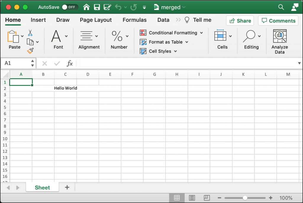
To get some hands-on experience, change the range of cells you want to merge and try it with and without the alignment set.
Now you are ready to learn about folding columns or rows!
Folding Rows and Columns
Microsoft Excel supports the folding of rows and columns. The term “folding” is also called “hiding” or creating an “outline”. The rows or columns that get folded can be unfolded (or expanded) to make them visible again. You can use this functionality to make a spreadsheet briefer. For example, you might want to only show the sub-totals or the results of equations rather than all of the data at once.
OpenPyXL supports folding too. To see how this works, create a new file named folding.py and enter the following code:
# folding.py

import openpyxl


def folding(path, rows=None, cols=None, hidden=True):
    workbook = openpyxl.Workbook()
    sheet = workbook.active

    if rows:
        begin_row, end_row = rows
        sheet.row_dimensions.group(begin_row, end_row, hidden=hidden)

    if cols:
        begin_col, end_col = cols
        sheet.column_dimensions.group(begin_col, end_col, hidden=hidden)

    workbook.save(path)


if __name__ == "__main__":
    folding("folded.xlsx", rows=(1, 5), cols=("C", "F"))
Your folding() function accepts a tuple of rows or columns or both. You can tell OpenPyXL whether or not you want those rows and columns to be hidden, or folded. In this example, you fold rows 1-5 and columns C-F. To cause the folding to occur, you need to call sheet.row_dimensions.group().
When you run this code, your spreadsheet will look like this:
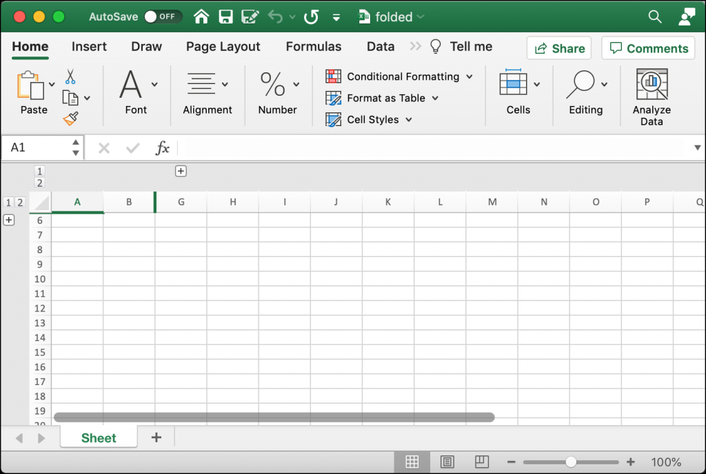
You can see in this spreadsheet that some of the rows and columns are folded or hidden. There is a “+” symbol next to row 6 and another “+” symbol above column “G”. If you click on either of those buttons, it will expand the folded rows or columns.
Give this code a try. You can also experiment with different row or column ranges.
Now you are ready to learn how to freeze a pane!
Freezing Panes
Microsoft Excel allows you to freeze panes. What that means is that you can freeze one or more columns or rows. One popular use case is to freeze a row of headers so that the headers are always visible while scrolling through a lot of data.
OpenPyXL provides a freeze_panes attribute on the Worksheet object that you can set. You need to select a cell below and to the right of the columns that you want to freeze. For example, if you want to freeze the first row in your spreadsheet, then you would select cell at “A2” to apply the freeze to that row.
You can see how this works by writing some code. Open up a new file and name it freezing_panes.py. Then enter the following into it:
# freezing_panes.py

from openpyxl import Workbook


def freeze(path, row_to_freeze):
    workbook = Workbook()
    sheet = workbook.active
    sheet.title = "Freeze"
    sheet.freeze_panes = row_to_freeze
    headers = ["Name", "Address", "State", "Zip"]
    sheet["A1"] = headers[0]
    sheet["B1"] = headers[1]
    sheet["C1"] = headers[2]
    sheet["D1"] = headers[3]
    data = [dict(zip(headers, ("Mike", "123 Storm Dr", "IA", "50000"))),
            dict(zip(headers, ("Ted", "555 Tornado Alley", "OK", "90000")))]
    row = 2
    for d in data:
        sheet[f'A{row}'] = d["Name"]
        sheet[f'B{row}'] = d["Address"]
        sheet[f'C{row}'] = d["State"]
        sheet[f'D{row}'] = d["Zip"]
        row += 1
    workbook.save(path)


if __name__ == "__main__":
    freeze("freeze.xlsx", row_to_freeze="A2")
Here you create a new Workbook and set the active sheet’s title to “Freeze”. Then you set the freeze_panes attribute to “A2”. The rest of the code in the function adds a couple of rows of data to the Worksheet.
When you run this code, the spreadsheet that you create will look like this:
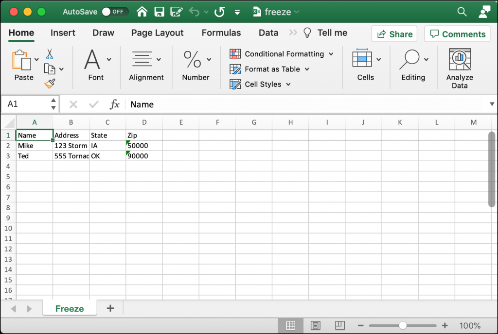
Try scrolling down through some rows in the spreadsheet. The top row should always remain visible because it has been “frozen”.
Wrapping Up
You can use OpenPyXL not only to create an Excel spreadsheet, but modify a pre-existing one. In this chapter, you learned how to do the following:
- Create a spreadsheet
- Write to a spreadsheet
- Add and remove sheets
- Insert and delete rows and columns
- Edit cell data
- Create merged cells
- Freeze panes
Give the examples in this chapter a try. Then modify them a bit to see what else you can do on your own.