
Combine text from two or more cells into one cell
You can combine data from multiple cells into a single cell using the Ampersand symbol (&) or the CONCAT function.

Combine data with the Ampersand symbol (&)
-
Select the cell where you want to put the combined data.
-
Type = and select the first cell you want to combine.
-
Type & and use quotation marks with a space enclosed.
-
Select the next cell you want to combine and press enter. An example formula might be =A2&» «&B2.
Combine data using the CONCAT function
-
Select the cell where you want to put the combined data.
-
Type =CONCAT(.
-
Select the cell you want to combine first.
Use commas to separate the cells you are combining and use quotation marks to add spaces, commas, or other text.
-
Close the formula with a parenthesis and press Enter. An example formula might be =CONCAT(A2, » Family»).
Need more help?

See also
TEXTJOIN function
CONCAT function
Merge and unmerge cells
CONCATENATE function
How to avoid broken formulas
Automatically number rows
Need more help?
Merge and unmerge cells
You can’t split an individual cell, but you can make it appear as if a cell has been split by merging the cells above it.
Merge cells
-
Select the cells to merge.
-
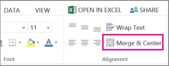
Select Merge & Center.
Important: When you merge multiple cells, the contents of only one cell (the upper-left cell for left-to-right languages, or the upper-right cell for right-to-left languages) appear in the merged cell. The contents of the other cells that you merge are deleted.
Unmerge cells
-
Select the Merge & Center down arrow.
-
Select Unmerge Cells.
Important:
-
You cannot split an unmerged cell. If you are looking for information about how to split the contents of an unmerged cell across multiple cells, see Distribute the contents of a cell into adjacent columns.
-
After merging cells, you can split a merged cell into separate cells again. If you don’t remember where you have merged cells, you can use the Find command to quickly locate merged cells.
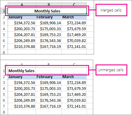
Merging combines two or more cells to create a new, larger cell. This is a great way to create a label that spans several columns.
In the example here, cells A1, B1, and C1 were merged to create the label “Monthly Sales” to describe the information in rows 2 through 7.
Merge cells
Merge two or more cells by following these steps:
-
Select two or more adjacent cells you want to merge.
Important: Ensure that the data you want to retain is in the upper-left cell, and keep in mind that all data in the other merged cells will be deleted. To retain any data from those other cells, simply copy it to another place in the worksheet—before you merge.
-
On the Home tab, select Merge & Center.

Tips:
-
If Merge & Center is disabled, ensure that you’re not editing a cell—and the cells you want to merge aren’t formatted as an Excel table. Cells formatted as a table typically display alternating shaded rows, and perhaps filter arrows on the column headings.
-
To merge cells without centering, click the arrow next to Merge and Center, and then click Merge Across or Merge Cells.
Unmerge cells
If you need to reverse a cell merge, click onto the merged cell and then choose Unmerge Cells item in the Merge & Center menu (see the figure above).
Split text from one cell into multiple cells
You can take the text in one or more cells, and distribute it to multiple cells. This is the opposite of concatenation, in which you combine text from two or more cells into one cell.
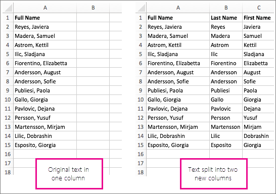
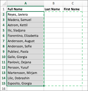
For example, you can split a column containing full names into separate First Name and Last Name columns:
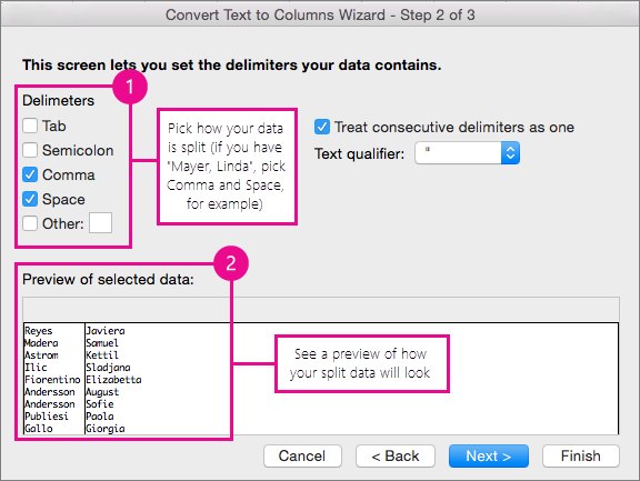
Follow the steps below to split text into multiple columns:
-
Select the cell or column that contains the text you want to split.
-
Note: Select as many rows as you want, but no more than one column. Also, ensure that are sufficient empty columns to the right—so that none of your data is deleted. Simply add empty columns, if necessary.
-
Click Data >Text to Columns, which displays the Convert Text to Columns Wizard.
-
Click Delimited > Next.
-
Check the Space box, and clear the rest of the boxes. Or, check both the Comma and Space boxes if that is how your text is split (such as «Reyes, Javiers», with a comma and space between the names). A preview of the data appears in the panel at the bottom of the popup window.
-
Click Next and then choose the format for your new columns. If you don’t want the default format, choose a format such as Text, then click the second column of data in the Data preview window, and click the same format again. Repeat this for all of the columns in the preview window.
-
Click the
button to the right of the Destination box to collapse the popup window. -
Anywhere in your workbook, select the cells that you want to contain the split data. For example, if you are dividing a full name into a first name column and a last name column, select the appropriate number of cells in two adjacent columns.
-
Click the
button to expand the popup window again, and then click the Finish button.
Merging combines two or more cells to create a new, larger cell. This is a great way to create a label that spans several columns. For example, here cells A1, B1, and C1 were merged to create the label “Monthly Sales” to describe the information in rows 2 through 7.
Merge cells
-
Click the first cell and press Shift while you click the last cell in the range you want to merge.
Important: Make sure only one of the cells in the range has data.
-
Click Home > Merge & Center.
If Merge & Center is dimmed, make sure you’re not editing a cell or the cells you want to merge aren’t inside a table.
Tip: To merge cells without centering the data, click the merged cell and then click the left, center or right alignment options next to Merge & Center.
If you change your mind, you can always undo the merge by clicking the merged cell and clicking Merge & Center.
Unmerge cells
To unmerge cells immediately after merging them, press Ctrl + Z. Otherwise do this:
-
Click the merged cell and click Home > Merge & Center.
The data in the merged cell moves to the left cell when the cells split.
Need more help?
You can always ask an expert in the Excel Tech Community or get support in the Answers community.
See Also
Overview of formulas in Excel
How to avoid broken formulas
Find and correct errors in formulas
Excel keyboard shortcuts and function keys
Excel functions (alphabetical)
Excel functions (by category)
Need more help?
Want more options?
Explore subscription benefits, browse training courses, learn how to secure your device, and more.
Communities help you ask and answer questions, give feedback, and hear from experts with rich knowledge.
Надпись на заборе: «Катя + Миша + Семён + Юра + Дмитрий Васильевич +
товарищ Никитин + рыжий сантехник + Витенька + телемастер Жора +
сволочь Редулов + не вспомнить имени, длинноволосый такой +
ещё 19 мужиков + муж = любовь!»
Способ 1. Функции СЦЕПИТЬ, СЦЕП и ОБЪЕДИНИТЬ
В категории Текстовые есть функция СЦЕПИТЬ (CONCATENATE), которая соединяет содержимое нескольких ячеек (до 255) в одно целое, позволяя комбинировать их с произвольным текстом. Например, вот так:

Нюанс: не забудьте о пробелах между словами — их надо прописывать как отдельные аргументы и заключать в скобки, ибо текст.
Очевидно, что если нужно собрать много фрагментов, то использовать эту функцию уже не очень удобно, т.к. придется прописывать ссылки на каждую ячейку-фрагмент по отдельности. Поэтому, начиная с 2016 версии Excel, на замену функции СЦЕПИТЬ пришла ее более совершенная версия с похожим названием и тем же синтаксисом — функция СЦЕП (CONCAT). Ее принципиальное отличие в том, что теперь в качестве аргументов можно задавать не одиночные ячейки, а целые диапазоны — текст из всех ячеек всех диапазонов будет объединен в одно целое:

Для массового объединения также удобно использовать новую функцию ОБЪЕДИНИТЬ (TEXTJOIN), появившуюся начиная с Excel 2016. У нее следующий синтаксис:
=ОБЪЕДИНИТЬ(Разделитель; Пропускать_ли_пустые_ячейки; Диапазон1; Диапазон2 … )
где
- Разделитель — символ, который будет вставлен между фрагментами
- Второй аргумент отвечает за то, нужно ли игнорировать пустые ячейки (ИСТИНА или ЛОЖЬ)
- Диапазон 1, 2, 3 … — диапазоны ячеек, содержимое которых хотим склеить
Например:

Способ 2. Символ для склеивания текста (&)
Это универсальный и компактный способ сцепки, работающий абсолютно во всех версиях Excel.
Для суммирования содержимого нескольких ячеек используют знак плюс «+«, а для склеивания содержимого ячеек используют знак «&» (расположен на большинстве клавиатур на цифре «7»). При его использовании необходимо помнить, что:
- Этот символ надо ставить в каждой точке соединения, т.е. на всех «стыках» текстовых строк также, как вы ставите несколько плюсов при сложении нескольких чисел (2+8+6+4+8)
- Если нужно приклеить произвольный текст (даже если это всего лишь точка или пробел, не говоря уж о целом слове), то этот текст надо заключать в кавычки. В предыдущем примере с функцией СЦЕПИТЬ о кавычках заботится сам Excel — в этом же случае их надо ставить вручную.
Вот, например, как можно собрать ФИО в одну ячейку из трех с добавлением пробелов:

Если сочетать это с функцией извлечения из текста первых букв — ЛЕВСИМВ (LEFT), то можно получить фамилию с инициалами одной формулой:

Способ 3. Макрос для объединения ячеек без потери текста.
Имеем текст в нескольких ячейках и желание — объединить эти ячейки в одну, слив туда же их текст. Проблема в одном — кнопка Объединить и поместить в центре (Merge and Center) в Excel объединять-то ячейки умеет, а вот с текстом сложность — в живых остается только текст из верхней левой ячейки.
Чтобы объединение ячеек происходило с объединением текста (как в таблицах Word) придется использовать макрос. Для этого откройте редактор Visual Basic на вкладке Разработчик — Visual Basic (Developer — Visual Basic) или сочетанием клавиш Alt+F11, вставим в нашу книгу новый программный модуль (меню Insert — Module) и скопируем туда текст такого простого макроса:
Sub MergeToOneCell()
    Const sDELIM As String = " "     'символ-разделитель
    Dim rCell As Range
    Dim sMergeStr As String
    If TypeName(Selection) <> "Range" Then Exit Sub   'если выделены не ячейки - выходим
    With Selection
        For Each rCell In .Cells
            sMergeStr = sMergeStr & sDELIM & rCell.Text  'собираем текст из ячеек
        Next rCell
        Application.DisplayAlerts = False   'отключаем стандартное предупреждение о потере текста
        .Merge Across:=False                'объединяем ячейки
        Application.DisplayAlerts = True
        .Item(1).Value = Mid(sMergeStr, 1 + Len(sDELIM))    'добавляем к объед.ячейке суммарный текст
    End With
End Sub
Теперь, если выделить несколько ячеек и запустить этот макрос с помощью сочетания клавиш Alt+F8 или кнопкой Макросы на вкладке Разработчик (Developer — Macros), то Excel объединит выделенные ячейки в одну, слив туда же и текст через пробелы.
Ссылки по теме
- Делим текст на куски
- Объединение нескольких ячеек в одну с сохранением текста с помощью надстройки PLEX
- Что такое макросы, как их использовать, куда вставлять код макроса на VBA

If you have a large worksheet in an Excel workbook in which you need to combine text from multiple cells, you can breathe a sigh of relief because you don’t have to retype all that text. You can easily concatenate the text.
Concatenate is simply a fancy way ot saying “to combine” or “to join together” and there is a special CONCATENATE function in Excel to do this. This function allows you to combine text from different cells into one cell. For example, we have a worksheet containing names and contact information. We want to combine the Last Name and First Name columns in each row into the Full Name column.
To begin, select the first cell that will contain the combined, or concatenated, text. Start typing the function into the cell, starting with an equals sign, as follows.
=CONCATENATE(

Now, we enter the arguments for the CONCATENATE function, which tell the function which cells to combine. We want to combine the first two columns, with the First Name (column B) first and then the Last Name (column A). So, our two arguments for the function will be B2 and A2.
There are two ways you can enter the arguments. First, you can type the cell references, separated by commas, after the opening parenthesis and then add a closing parenthesis at the end:
=CONCATENATE(B2,A2)
You can also click on a cell to enter it into the CONCATENATE function. In our example, after typing the name of the function and the opening parenthesis, we click on the B2 cell, type a comma after B2 in the function, click on the A2 cell, and then type the closing parenthesis after A2 in the function.
Press Enter when you’re done adding the cell references to the function.
Notice that there is no space in between the first and last name. That’s because the CONCATENATE function combines exactly what’s in the arguments you give it and nothing more. There is no space after the first name in B2, so no space was added. If you want to add a space, or any other punctuation or details, you must tell the CONCATENATE function to include it.
To add a space between the first and last names, we add a space as another argument to the function, in between the cell references. To do this, we type a space surrounded by double quotes. Make sure the three arguments are separated by commas.
=CONCATENATE(B2," ",A2)
Press Enter.
That’s better. Now, there is a space between the first and last names.
RELATED: How to Automatically Fill Sequential Data into Excel with the Fill Handle
Now, you’re probably thinking you have to type that function in every cell in the column or manually copy it to each cell in the column. Actually, you don’t. We’ve got another neat trick that will help you quickly copy the CONCATENATE function to the other cells in the column (or row). Select the cell in which you just entered the CONCATENATE function. The small square on the lower-right corner of the selected is called the fill handle. The fill handle allows you to quickly copy and paste content to adjacent cells in the same row or column.
Move your cursor over the fill handle until it turns into a black plus sign and then click and drag it down.
The function you just entered is copied down to the rest of the cells in that column, and the cell references are changed to match the row number for each row.
You can also concatenate text from multiple cells using the ampersand (&) operator. For example, you can enter =B2&" "&A2 to get the same result as =CONCATENATE(B2," ",A2) . There’s no real advantage of using one over the other. although using the ampersand operator results in a shorter entry. However, the CONCATENATE function may be more readable, making it easier to understand what’s happening in the cell.
READ NEXT
- › How to Merge Two Columns in Microsoft Excel
- › How to Add Text With a Formula in Google Sheets
- › How to Add Text to a Cell With a Formula in Excel
- › How to Concatenate in Microsoft Excel
- › How to Combine Data From Spreadsheets in Microsoft Excel
- › 12 Basic Excel Functions Everybody Should Know
- › How to Calculate Age in Microsoft Excel
- › Google Chrome Is Getting Faster
How-To Geek is where you turn when you want experts to explain technology. Since we launched in 2006, our articles have been read billions of times. Want to know more?
Merged cells are one of the most popular options used by beginner spreadsheet users.
But they have a lot of drawbacks that make them a not so great option.
In this post, I’ll show you everything you need to know about merged cells including 8 ways to merge cells.
I’ll also tell you why you shouldn’t use them and a better alternative that will produce the same visual result.
What is a Merged Cell
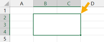
A merged cell in Excel combines two or more cells into one large cell. You can only merge contiguous cells that form a rectangular shape.
The above example shows a single merged cell resulting from merging 6 cells in the range B2:C4.
Why You Might Merge a Cell
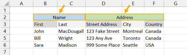
Merging cells is a common technique used when a title or label is needed for a group of cells, rows or columns.
When you merge cells, only the value or formula in the top left cell of the range is preserved and displayed in the resulting merged cell. Any other values or formulas are discarded.
The above example shows two merged cells in B2:C2 and D2:F2 which indicates the category of information in the columns below. For example the First and Last name columns are organized with a Name merged cell.
Why is the Merge Command Disabled?
On occasion, you might find the Merge & Center command in Excel is greyed out and not available to use.
There are two reasons why the Merge & Center command can become unavailable.
- You are trying to merge cells inside an Excel table.
- You are trying to merge cells in a protected sheet.
Cells inside an Excel table can not be merged and there is no solution to enable this.
If most of the other commands in the ribbon are greyed out too, then it’s likely the sheet is protected. In order to access the Merge option, you will need to unprotect the worksheet.
This can be done by going to the Review tab and clicking the Unprotect Sheet command.
If the sheet has been protected with a password, then you will need to enter it in order to unprotect the sheet.
Now you should be able to merge cells inside the sheet.
Merged Cells Only Retain the Top Left Values
Warning before you start merging cells!
If the cells contain data or formulas, then you will lose anything not in the upper left cell.
A warning dialog box will appear telling you Merging cells only keeps the upper-left value and discards other values.
The above example shows the result of merging cells B2:C4 which contains text data. Only the data from cell B2 remains in the resulting merged cells.
If no data is present in the selected cells, then no warning will appear when trying to merge cells.
8 Ways to Merge a Cell
Merging cells is an easy task to perform and there are a variety of places this command can be found.
Merge Cells with the Merge & Center Command in the Home Tab
The easiest way to merge cells is using the command found in the Home tab.
- Select the cells you want to merge together.
- Go to the Home tab.
- Click on the Merge & Center command found in the Alignment section.
Merge Cells with the Alt Hotkey Shortcut
There is an easy way to access the Home tab Merge and Center command using the Alt key.
Press Alt H M C in sequence on your keyboard to use the Merge & Center command.
Merge Cells with the Format Cells Dialog Box
Merging cells is also available from the Format Cells dialog box. This is the menu which contains all formatting options including merging cells.
You can open the Format Cells dialog box a few different ways.
- Go to the Home tab and click on the small launch icon in the lower right corner of the Alignment section.
- Use the Ctrl + 1 keyboard shortcut.
- Right click on the selected cells and choose Format Cells.
Go to the Alignment tab in the Format Cells menu then check the Merge cells option and press the OK button.
Merge Cells with the Quick Access Toolbar
If you use the Merge & Center command a lot, then it might make sense to add it to the Quick Access Toolbar so it’s always readily available to use.
Go to the Home tab and right click on the Merge & Center command then choose Add to Quick Access Toolbar from the options.
This will add the command to your QAT which is always available to use.
A nice bonus that comes with the quick access command is it gets its own hotkey shortcut based on its position in the QAT. When you press the Alt key, Excel will show you what key to press next in order to access the command.
In the above example, the Merge and Center command is the third command in the QAT so the hotkey shortcut is Alt 3.
Merge Cells with Copy and Paste
If you have a merged cell in your sheet already then you can copy and paste it to create more merged cells. This will produce merged cells with the exact same dimensions.
Copy a merged cell using Ctrl + C then paste it into a new location using Ctrl + V. Just make sure the paste area doesn’t overlap an existing merged cell.
Merge Cells with VBA
Sub MergeCells()
    Range("B2:C4").Merge
End Sub
The basic command for merging cells in VBA is quite simple. The above code will merge cells B2:C4.
Merge Cells with Office Scripts
function main(workbook: ExcelScript.Workbook) {
	let selectedSheet = workbook.getActiveWorksheet();
	selectedSheet.getRange("B2:C4").merge(false);
	selectedSheet.getRange("B2:C4").getFormat().setHorizontalAlignment(ExcelScript.HorizontalAlignment.center);
}
The above office script will merge and center the range B2:C4.
Merge Cells inside a PivotTable
We can’t make this change for the selected cells because it will affect a PivotTable. Use the field list to change the report. If you are trying to insert or delete cells, move the PivotTable and try again.
If you try to use the Merge and Center command inside a Pivot Table, you will be greeted with the above error message.
You can’t use the Merge & Center command inside a PivotTable, but there is a way to merge cells in the PivotTable options menu.
In order to avail of this option, you will first need to make sure your Pivot Table is in the tabular display mode.
- Select a cell inside your PivotTable.
- Go to the Design tab.
- Click on Report Layout.
- Choose Show in Tabular Form.
Your pivot table will now be in the tabular form where each field you add to the Rows area will be in its own column with data in a displayed in a single row.
Now you can enable the option to show merge cells inside the pivot table.
- Select a cell inside your PivotTable.
- Go to the PivotTable Analyze tab.
- Click on Options.
This will open up the PivotTable Options menu.
Enable the Merge and center cells with labels setting in the PivotTable Options menu.
- Click on the Layout & Format tab.
- Check the Merge and center cells with labels option.
- Press the OK button.
Now as you expand and collapse fields in your pivot table, fields will merge when they have a common label.
10 Ways to Unmerge a Cell
Unmerging a cell is also quick and easy. Most methods involve the same steps as used to merge the cell, but there are a few extra methods worth knowing.
Unmerge Cells with the Home Tab Command
This is the same process as merging cells from the Home tab command.
- Select the merged cells to unmerge.
- Go to the Home tab.
- Click on the Merge & Center command.
Unmerge Cells with the Format Cells Menu
You can unmerge cells from the Format Cells dialog box as well.
Press Ctrl + 1 to open the Format Cells menu then go to the Alignment tab then uncheck the Merge cells option and press the OK button.
Unmerge Cells with the Alt Hot Key Shortcut
You can use the same Alt hot key combination to unmerge a merged cell. Select the merged cell you want to unmerge then press Alt H M C in sequence to unmerge the cells.
Unmerge Cells with Copy and Paste
You can copy the format from a regular single cell to unmerge merged cells.
Find a single cell and use Ctrl + C to copy it, then select the merged cells and press Ctrl + V to paste the cell.
You can use the Paste Special options to avoid overwriting any data when pasting. Press Ctrl + Alt + V then select the Formats option.
Unmerge Cells with the Quick Access Toolbar
This is a great option if you have already added the Merge & Center command to the quick access toolbar previously.
All you need to do is select the merged cells and click on the command or use the Alt hot key shortcut.
Unmerge Cells with the Clear Formats Command
Merged cells are a type of format, so it’s possible to unmerge cells by clearing the format from the cell.
- Select the merged cell to unmerge.
- Go to the Home tab.
- Click on the right part of the Clear button found in the Editing section.
- Select Clear Formats from the options.
Unmerge Cells with VBA
Sub UnMergeCells()
    Range("B2:C4").UnMerge
End Sub
Above is the basic command for unmerging cells in VBA. This will unmerge cells B2:C4.
Unmerge Cells with Office Scripts
Most methods of merging a cell can be performed again to unmerge cells like a toggle switch to merge or unmerge.
However the code in office scripts doesn’t work like this and instead, you will need to remove formatting to unmerge.
function main(workbook: ExcelScript.Workbook) {
	let selectedSheet = workbook.getActiveWorksheet();
	selectedSheet.getRange("B2:C4").clear(ExcelScript.ClearApplyTo.formats);
}
The above code will clear the format in cells B2:C4 and unmerge any merged cells it contains.
Unmerge Cells with the Accessibility Pane
Merged cells create problems for screen readers which is an accessibility issue. Because of this, they are flagged in the Accessibility window pane.
If you know the location of the merged cells, you can select them and go to the Review tab then click on the lower part of the Check Accessibility button and choose Unmerge Cells.
If you don’t know where all the merged cells are, you can open up the accessibility pane and it will show you where there are and you will be able to unmerge them one by one.
Go to the Review tab and click on the top part of the Check Accessibility command to launch the accessibility window pane.
This will show a Merged Cells section which you can expand to see all merged cells in the workbook. Click on the address and Excel will take you to that location.
Click on the downward chevron icon to the right of the address and the Unmerge option can be selected.
Unmerge Cells inside a PivotTable
To unmerge cells inside a pivot table, you just need to disable the setting in the pivot table options menu.
Now you can enable the option to show merge cells inside the pivot table.
- Select a cell inside your PivotTable.
- Go to the PivotTable Analyze tab.
- Click on Options.
- Click on the Layout & Format tab.
- Uncheck the Merge and center cells with labels option.
- Press the OK button.
Merge Multiple Ranges in One Step
In Excel, you can select multiple non-continuous ranges in a sheet by holding the Ctrl key. A nice consequence of this is you can convert these multiple ranges into merged cells in one step.
Hold the Ctrl key while selecting multiple ranges with the mouse. When you’re finished selecting the ranges you can release the Ctrl key and then go to the Home tab and click on the Merge & Center command.
Each range will become its own merged cell.
Combine Data Before Merging Cells
Before you merge any cells which contain data, it’s advised to combine the data since only the data in the top left cell is preserved when merging cells.
There are a variety of ways to do this, but using the TEXTJOIN function is among the easiest and most flexible as it will allow you to separate each cell’s data using a delimiter if needed.
= TEXTJOIN ( ", ", TRUE, B2:C4 )The above formula will join all the text in range B2:C4 going from left to right and then top to bottom. Text in each cell is separated with a comma and space.
Once you have the formula result, you can copy and paste it as a value so that the data is retained when you merge the cells.
How to Get Data from Merged Cells in Excel
A common misconception is that each cell of in the merged range contains the data entered inside.
In fact, only the top left cell will contain any data.
In the above example, the formula references the top left value in the merged range. The result returned is what is seen in the merged range.
In this example, the formula references a cell that is not the top left most cell in the merged range. The result is 0 because this cell is empty and contains no value.
In order to extract data from a merged range, you will always need to reference the top left most cell of the range. Fortunately, Excel automatically does this for you when you select the merged cell in a formula.
How to Find Merged Cells in a Workbook
If you create a bunch of merged cells, you might need to find them all later. Thankfully it’s not a painful process.
This can be done using the Find & Select command.
Go to the Home tab and click on the Find & Select button found in the Editing section, then choose the Find option. This will open the Find and Replace menu
You can also use the Ctrl + F keyboard shortcut.
You don’t need to enter any text to find, you can use this menu to find cells formatted as merged cells.
- Click on the Format button to open the Find Format menu.
- Go to the Alignment tab.
- Check the Merge cells option.
- Press the OK button in the Find Format menu.
- Press the Find All or Find Next button in the Find and Replace menu.
Unmerge All Merged Cells
Fortunately, unmerging all merged cells in a sheet is very easy.
- Select the entire sheet. You can do this two ways.
- Click on the select all button where the column headings meet the row headings.
- Press Ctrl + A on your keyboard.
- Go to the Home tab.
- Press the Merge & Center command.
This will unmerge all the merged cells and leave all the other cells unaffected.
Why You Shouldn’t Merge Cells
There are a lot of reasons why you shouldn’t merge cells.
- You can’t sort data with merged cells.
- You can’t filter data with merged cells.
- You can’t copy and paste values into merged cells.
- It will create accessibility problems for screen readers by changing the order in which text should be read.
This isn’t an exhaustive list, there are likely many more you will come across should you choose to merge cells.
Alternative to Merging a Cell
Good news!
There is a much better alternative than merging cells.
This alternative has none of the negative features that come with merging cells but will still allow you to achieve the same visual look of a merged cell.
It will allow you to display text centered across a range of cells without merging the cells.
Unfortunately, this technique will only work horizontally with one row of cells. There is no option to do something similar with a vertical range of cells.
Select the horizontal range of cells that you would like to center your text across. The first cell should contain the text which is to be centered while the remaining cells should be empty.
This example shows text in cell B2 and the range B2:C2 is selected as the range to center across.
Go to the Home tab and click on the small launch icon in the lower right corner of the Alignment section. This will open up the Format Cells dialog box with the Alignment tab active.
You can also press Ctrl + 1 to open the Format Cells dialog box and navigate to the Alignment tab.
Select Center Across Selection from the Horizontal dropdown options in the Text alignment section.
The text will now appear as though it occupies all cells but it will only exist in the first cell of the centering selection and each cell is still separate.
Pros
- The text appears centered across the selected range similar to a merged cell.
- No negative effects from merged cells.
- Can be used inside an Excel table.
Cons
- Can not center across a vertical range of cells.
Conclusions
There are lots of ways to merge cells in Excel. You can also easily unmerge cells too if you need to.
There are many things to consider when merging cells in Excel.
As you have seen, there are lots of pitfalls to merged cells that you should consider before implementing them in your workbooks.
Do you have a favorite merge method or warning about the dangers of merged cells that are not listed in the post? Let me know about it in the comments.
About the Author
John is a Microsoft MVP and qualified actuary with over 15 years of experience. He has worked in a variety of industries, including insurance, ad tech, and most recently Power Platform consulting. He is a keen problem solver and has a passion for using technology to make businesses more efficient.
Содержание
- Merge and unmerge cells
- Merge cells
- Unmerge cells
- Merge cells
- Unmerge cells
- Split text from one cell into multiple cells
- Merge cells
- Unmerge cells
- Need more help?
- TEXTJOIN function
- Syntax
- Remarks
- Examples
- TEXTJOIN function in Excel to merge text from multiple cells into one
- Excel TEXTJOIN function
- TEXTJOIN in Excel — 6 things to remember
- How to join text in Excel — formula examples
- Convert column to comma separated list
- Join cells with different delimiters
- Join text and dates in Excel
- Merge text with line breaks
- TEXTJOIN IF to merge text with conditions
- Lookup and return multiple matches in comma separated list
- Excel TEXTJOIN not working
- Available downloads
- You may also be interested in
Merge and unmerge cells
You can’t split an individual cell, but you can make it appear as if a cell has been split by merging the cells above it.
Merge cells
Select the cells to merge.
Select Merge & Center.
Important: When you merge multiple cells, the contents of only one cell (the upper-left cell for left-to-right languages, or the upper-right cell for right-to-left languages) appear in the merged cell. The contents of the other cells that you merge are deleted.
Unmerge cells
Select the Merge & Center down arrow.
Select Unmerge Cells.
You cannot split an unmerged cell. If you are looking for information about how to split the contents of an unmerged cell across multiple cells, see Distribute the contents of a cell into adjacent columns.
After merging cells, you can split a merged cell into separate cells again. If you don’t remember where you have merged cells, you can use the Find command to quickly locate merged cells.
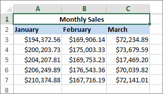
Merging combines two or more cells to create a new, larger cell. This is a great way to create a label that spans several columns.
In the example here, cells A1, B1, and C1 were merged to create the label “Monthly Sales” to describe the information in rows 2 through 7.
Merge cells
Merge two or more cells by following these steps:
Select two or more adjacent cells you want to merge.
Important: Ensure that the data you want to retain is in the upper-left cell, and keep in mind that all data in the other merged cells will be deleted. To retain any data from those other cells, simply copy it to another place in the worksheet—before you merge.
On the Home tab, select Merge & Center.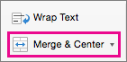
If Merge & Center is disabled, ensure that you’re not editing a cell—and the cells you want to merge aren’t formatted as an Excel table. Cells formatted as a table typically display alternating shaded rows, and perhaps filter arrows on the column headings.
To merge cells without centering, click the arrow next to Merge and Center, and then click Merge Across or Merge Cells.
Unmerge cells
If you need to reverse a cell merge, click onto the merged cell and then choose Unmerge Cells item in the Merge & Center menu (see the figure above).
Split text from one cell into multiple cells
You can take the text in one or more cells, and distribute it to multiple cells. This is the opposite of concatenation, in which you combine text from two or more cells into one cell.
For example, you can split a column containing full names into separate First Name and Last Name columns:
Follow the steps below to split text into multiple columns:
Select the cell or column that contains the text you want to split.
Note: Select as many rows as you want, but no more than one column. Also, ensure that are sufficient empty columns to the right—so that none of your data is deleted. Simply add empty columns, if necessary.
Click Data > Text to Columns, which displays the Convert Text to Columns Wizard.
Click Delimited > Next.
Check the Space box, and clear the rest of the boxes. Or, check both the Comma and Space boxes if that is how your text is split (such as «Reyes, Javiers», with a comma and space between the names). A preview of the data appears in the panel at the bottom of the popup window.
Click Next and then choose the format for your new columns. If you don’t want the default format, choose a format such as Text, then click the second column of data in the Data preview window, and click the same format again. Repeat this for all of the columns in the preview window.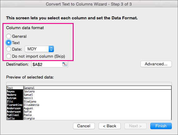
Click the  button to the right of the Destination box to collapse the popup window.
Anywhere in your workbook, select the cells that you want to contain the split data. For example, if you are dividing a full name into a first name column and a last name column, select the appropriate number of cells in two adjacent columns.
Click the  button to expand the popup window again, and then click the Finish button.

Merging combines two or more cells to create a new, larger cell. This is a great way to create a label that spans several columns. For example, here cells A1, B1, and C1 were merged to create the label “Monthly Sales” to describe the information in rows 2 through 7.
Merge cells
Click the first cell and press Shift while you click the last cell in the range you want to merge.
Important: Make sure only one of the cells in the range has data.
Click Home > Merge & Center.
If Merge & Center is dimmed, make sure you’re not editing a cell or the cells you want to merge aren’t inside a table.
Tip: To merge cells without centering the data, click the merged cell and then click the left, center or right alignment options next to Merge & Center.
If you change your mind, you can always undo the merge by clicking the merged cell and clicking Merge & Center .
Unmerge cells
To unmerge cells immediately after merging them, press Ctrl + Z. Otherwise do this:
Click the merged cell and click Home > Merge & Center.
The data in the merged cell moves to the left cell when the cells split.
Need more help?
You can always ask an expert in the Excel Tech Community or get support in the Answers community.
Источник
TEXTJOIN function
The TEXTJOIN function combines the text from multiple ranges and/or strings, and includes a delimiter you specify between each text value that will be combined. If the delimiter is an empty text string, this function will effectively concatenate the ranges.
Note: This feature is available on Windows or Mac if you have Office 2019, or if you have a Microsoft 365 subscription. If you are a Microsoft 365 subscriber, make sure you have the latest version of Office.
Syntax
TEXTJOIN(delimiter, ignore_empty, text1, [text2], …)
A text string, either empty, or one or more characters enclosed by double quotes, or a reference to a valid text string. If a number is supplied, it will be treated as text.
If TRUE, ignores empty cells.
Text item to be joined. A text string, or array of strings, such as a range of cells.
Additional text items to be joined. There can be a maximum of 252 text arguments for the text items, including text1. Each can be a text string, or array of strings, such as a range of cells.
For example, =TEXTJOIN(» «,TRUE, «The», «sun», «will», «come», «up», «tomorrow.») will return The sun will come up tomorrow.
If the resulting string exceeds 32767 characters (cell limit), TEXTJOIN returns the #VALUE! error.
Examples
Copy the example data in each of the following tables, and paste it in cell A1 of a new Excel worksheet. For formulas to show results, select them, press F2, and then press Enter. If you need to, you can adjust the column widths to see all the data.
Источник
TEXTJOIN function in Excel to merge text from multiple cells into one
 by Svetlana Cheusheva, updated on March 14, 2023
The tutorial shows how to use the TEXTJOIN function to merge text in Excel with practical examples.
Until recently, there were two prevalent methods to merge cell contents in Excel: the concatenation operator and CONCATENATE function. With the introduction of TEXTJOIN, it seems like a more powerful alternative has appeared, which enables you to join text in a more flexible manner including any delimiter in between. But in truth, there’s much more to it!
Excel TEXTJOIN function
TEXTJOIN in Excel merges text strings from multiple cells or ranges and separates the combined values with any delimiter that you specify. It can either ignore or include empty cells in the result.
The function is available in Excel for Office 365, Excel 2021, and Excel 2019.
The syntax of the TEXTJOIN function is as follows:
- Delimiter (required) — is a separator between each text value that you combine. Usually, it is supplied as a text string enclosed in double quotes or a reference to a cell containing a text string. A number supplied as a delimiter is treated as text.
- Ignore_empty (required) — Determines whether to ignore empty cells or not:
- TRUE — ignore any blank cells.
- FALSE — include empty cells in the resulting string.
- Text1 (required) — first value to join. Can be supplied as a text string, a reference to a cell containing a string, or array of strings such as a range of cells.
- Text2, … (optional) — additional text values to be joined together. A maximum of 252 text arguments are allowed, including text1.
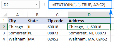
As an example, let’s combine address parts from cells B2, C2 and D2 together into one cell, separating the values with a comma and a space:
With the CONCATENATE function, you’d need to specify each cell individually and put a delimiter («, «) after each reference, which might be bothersome when merging the contents of many cells:
=CONCATENATE(A2, «, «, B2, «, «, C2)
With Excel TEXTJOIN, you specify the delimiter just once in the first argument, and supply a range of cells for the third argument:
=TEXTJOIN(«, «, TRUE, A2:C2)
TEXTJOIN in Excel — 6 things to remember
To effectively use TEXTJOIN in your worksheets, there are a few important points to take notice of:
- TEXTJOIN is a new function, which is only available in Excel 2019 — Excel 365. In earlier Excel versions, please use the CONCATENATE function or the «&» operator instead.
- In new versions if Excel, you can also use the CONCAT function to concatenate values from separate cells and ranges, but with no options for delimiters or empty cells.
- Any number supplied to TEXTJOIN for the delimiter or text arguments is converted to text.
- If delimiter is not specified or is an empty string («»), text values are concatenated without any delimiter.
- The function can handle up to 252 text arguments.
- The resulting string can contain a maximum of 32,767 characters, which is the cell limit in Excel. If this limit is exceeded, a TEXTJOIN formula returns the #VALUE! error.
How to join text in Excel — formula examples
To better understand all the advantages of TEXTJOIN, let’s take a look at how to use the function in real-life scenarios.
Convert column to comma separated list
When you are looking to concatenate a vertical list separating the values by a comma, semicolon or any other delimiter, TEXTJOIN is the right function to use.
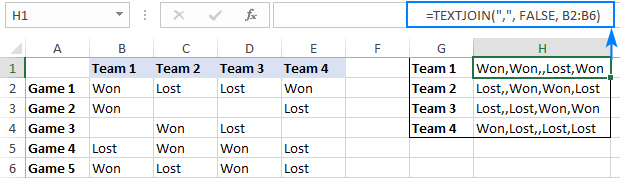
For this example, we’ll be concatenating wins and losses of each team from the table below. This can be done with the following formulas, which differ only in the range of cells that are joined.
=TEXTJOIN(«,», FALSE, B2:B6)
=TEXTJOIN(«,», FALSE, C2:C6)
In all the formulas, the following arguments are used:
- Delimiter — a comma («,»).
- Ignore_empty is set to FALSE to include empty cells because we need to show which games were not played.
As the result, you will get four comma-separated lists that represent wins and losses of each team in a compact form:
Join cells with different delimiters
In a situation when you need to separate the combined values with different delimiters, you can either supply several delimiters as an array constant or input each delimiter in a separate cell and use a range reference for the delimiter argument.
Supposing you want to join cells containing different name parts and get the result in this format: Last name, First name Middle name.
As you can see, the Last name and First name are separated by a comma and a space («, «) while the First name and Middle name by a space (» «) only. So, we include these two delimiters in an array constant <«, «,» «>and get the following formula:
Where A2:C2 are the name parts to be combined.
Alternatively, you can type the delimiters without quotation marks in some empty cells (say, a comma and a space in F3 and a space in G3) and use the range $F$3:$G$3 (please mind the absolute cell references) for the delimiter argument:
=TEXTJOIN($F$3:$G$3, TRUE, A2:C2)

By using this general approach, you can merge cell contents in various forms.
For example, if you want the result in the First name Middle initial Last name format, then use the LEFT function to extract the first character (the initial) from cell C2. As for the delimiters, we put a space (» «) between the First name and the Middle initial; a period and a space («. «) between the Initial and the Last name:
=TEXTJOIN(<» «,». «>, TRUE, B2, LEFT(C2,1), A2)

Join text and dates in Excel
In a specific case when you are merging text and dates, supplying dates directly to a TEXTJOIN formula won’t work. As you may remember, Excel stores dates as serial numbers, so your formula will return a number representing the date as shown in the screenshot below:
=TEXTJOIN(» «, TRUE, A2:B2)

To fix this, you need to convert the date into a text string before joining it. And here the TEXT function with the desired format code («mm/dd/yyyy» in our case) comes in handy:
=TEXTJOIN(» «, TRUE, A2, TEXT(B2, «mm/dd/yyyy»))

Merge text with line breaks
If you’d like to merge text in Excel so that each value starts in a new line, use CHAR(10) as the delimiter (where 10 is a linefeed character).
For example, to combine text from cells A2 and B2 separating the values by a line break, this is the formula to use:
=TEXTJOIN(CHAR(10), TRUE, A2:B2)

Tip. For the result to display in multiple lines like shown in the screenshot above, make sure the Wrap text feature is turned on.
TEXTJOIN IF to merge text with conditions
Due to the ability of Excel TEXTJOIN to handle arrays of strings, it can also be used to conditionally merge the contents of two or more cells. To have it done, use the IF function to evaluate a range of cells and return an array of values that meet the condition to the text1 argument of TEXTJOIN.
From the table shown in the screenshot below, suppose you wish to retrieve a list of Team 1 members. To achieve this, nest the following IF statement into the text1 argument:
In plain English, the above formula says: If column B equals 1, return a value from column A in the same row; otherwise return an empty string.
The complete formula for Team 1 takes this shape:
In a similar manner, you can get a comma-separated list of the members of Team 2:

Note. Due to the Dynamic Arrays feature available in Excel 365 and 2021, this works as a regular formula, shown in the screenshot above. In Excel 2019, you must enter it as a traditional array formula by pressing the Ctrl + Shift + Enter shortcut.
Lookup and return multiple matches in comma separated list
As you probably know, the Excel VLOOKUP function can only return the first found match. But what if you need to get all matches for a specific ID, SKU, or something else?
To output the results in separate cells, use one of the formulas described in How to VLOOKUP multiple values in Excel.
To look up and return all matching values in a single cell as a comma-separated list, use the TEXTJOIN IF formula.
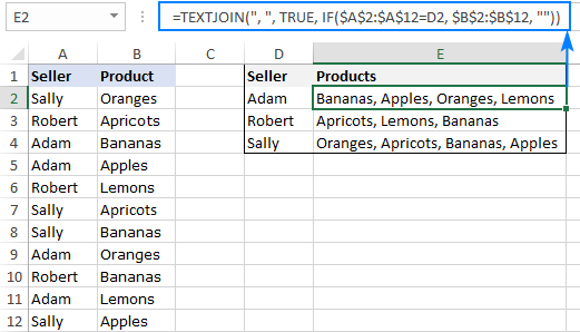
To see how it works in practice, let’s retrieve a list of products purchased by a given seller from the sample table below. This can be easily done with the following formula:
=TEXTJOIN(«, «, TRUE, IF($A$2:$A$12=D2, $B$2:$B$12, «»))
Where A2:A12 are seller names, B2:B12 are products, and D2 is the seller of interest.
The above formula goes to E2 and brings all the matches for the target seller in D2 (Adam). Due to the clever use of relative (for the target seller) and absolute (for the seller names and products) cell references, the formula correctly copies to the below cells and works nicely for the other two sellers too:
Note. As with the previous example, this works as a regular formula in Excel 365 and 2021, and as a CSE formula (Ctrl + Shift + Enter ) in Excel 2019.
The formula’s logic is exactly the same as in the previous example:
The IF statement compares each name in A2:A12 against the target name in D2 (Adam in our case):
If the logical test evaluates to TRUE (i.e. the name in D2 matches the name in column A), the formula returns a product from column B; otherwise an empty string («») is returned. The result of IF is the following array:
The array goes to the TEXTJOIN function as the text1 argument. And because TEXTJOIN is configured to separate the values with a comma and a space («, «), we get this string as the final result:
Bananas, Apples, Oranges, Lemons
Excel TEXTJOIN not working
When your TEXTJOIN formula results in an error, it’s most likely to be one of the following:
- #NAME? error occurs when TEXTJOIN is used in an older version of Excel where this function is not supported (pre-2019) or when the function’s name is misspelled.
- #VALUE! error occurs if the resulting string exceeds 32,767 characters.
- #VALUE! error may also occur if Excel does not recognize the delimiter as text, for example if you supply some non-printable character such as CHAR(0).
That’s how to use the TEXTJOIN function in Excel. I thank you for reading and hope to see you on our blog next week!
Available downloads
You may also be interested in
Table of contents
Can you have a dynamic delimiter?
I want to join text like a sentence from a list of items. I want the items to be combined using «,» but the last item should be combined with «, &». However long my list is the last item should be combined with the later.
Hello!
Use the TEXTBEFORE and TEXTAFTER functions to insert the desired character after the last comma.
I hope it’ll be helpful.
Do you know if it’s possible to combine the line break delimiter with finding multiple matches?
I tried this, but it doesn’t function properly, with or without the CSE:
=TEXTJOIN(CHAR(10), TRUE, IF($A$2:$A$12=D2, $B$2:$B$12, «»))
Hello!
I don’t really understand what you want to do. But maybe you will find this article useful: How to VLOOKUP multiple values in Excel with criteria. If this does not help, explain the problem in detail.
Hello!
Can you use TEXTJOIN in multiple sheets?, example: TEXTJOIN(«, «,TRUE,IF($C9=’5-Sale’!$D$10:$D$10009,’5-Sale’!$H$10:$H$10009,»»))). I use this formula and it displayed #VALUE. can you fix this or any advice?
Hope to hear from you soon. Thank you!!
Hello!
Perhaps the error occurs because the TEXJOIN function can join no more than 252 text arguments.
Please help with suitable formula:
Input in 3 columns:
A B C
Morning Adam Good
Afternoon Bob
Evening James
Alice
Sam
Pete
Desired Result in Column continuous sentences:
Good Morning Adam
Good Morning Bob
Good Morning James
Good Morning Alice
Good Morning Sam
Good Morning Pete
Good Afternoon Adam
Good Afternoon Bob
Good Afternoon James
Good Afternoon Alice
Good Afternoon Sam
Good Afternoon Pete
Good Evening Adam
Good Evening Bob
Good Evening James
Good Evening Alice
Good Evening Sam
Good Evening Pete
Using excel how to get the output from the below input
Name Task
a 1,2,3,4
b 5,6,7,8
c 9,10,11,12
d 13,14,15,16
Name Test
a 1
a 2
a 3
a 4
b 5
b 6
b 7
b 8
c 9
c 10
c 11
c 12
d 13
d 14
d 15
d 16
How to retain formatting of specific cell or cells while textjoin — for example: out of three cells being joined, only one was bold. In the textjoin cell, I want that value to retain its bold formating
Hi!
Excel formulas cannot change cell formatting. This can be done using a VBA macro.
i’ve been trying using formula’s to merge the bundle_Id values in one cell which have similar number to the different sheet but I am not able to merge them. Using =TEXTJOIN(«,»,true,B2:B9) and which is working well but have to merge the cells individually. Can you please suggest some formula on this.
Example —
bundle_id sku formula
1 75613 1
1 75176 1
1 74207 1
1 74301 1
1 62750 1
1 74378 1
1 74299 1
1 37738 1
2 75613 1
2 75176 1
2 74205 1
2 74301 1
2 62750 1
2 74378 1
2 74299 1
2 37738 1
Just like this i want to merge all 2 values in one column for 4000 row together. How can i merge them
Hi!
I am not sure I fully understand what you mean. If I understand correctly, your example has 3 values per line. Explain what you want to merge. Write an example of the result.
Hi,
I have an SAP extract for Special Instructions.
In SAP, for the same Special Instruction, I may have 1 or more lines of text and those lines need to be grouped into a single cell for each unique Customer ID.
What I need to do is combine the cells with a formula (which is the easy part) but I want to the formula to detect when the ID in column A changes to another accountID.
So 6 lines of data in Cell C1to C6 are combined and the formula detects that the ID changes to a new ID (from 10000 to 10001) and combines cells C7 to C9, and then C10 to C15.
Cust# Text ID Remit To Text
10000 0009 Remit to:
10000 0009 PERKINELMER Optoelectronics
10000 0009 c/o ROYAL BANK OF CANADA
10000 0009 1, Place Ville Marie
10000 0009 MontrГ©al (QC) H3C 3A7, Canada
10000 0009 Account #403
10001 0009 Remit to: EG&G Optoelectronics
10001 0009 P.O. Box 66512 AMS O’Hare
10001 0009 Chicago, IL 60666-0512 USA
10002 0009 Remit to: EG&G Optoelectronics
10002 0009 P.O. Box 66512 AMS O’Hare
10002 0009 Chicago, IL 60666-0512 USA
10003 0009 Remit to:
10003 0009 EG&G CANADA Ltd. Optoelectronics
10003 0009 c/o ROYAL BANK OF CANADA
10003 0009 1, Place Ville Marie
10003 0009 MontrГ©al (QC) H3C 3A7, Canada
10003 0009 Account #124
Hope this makes sense! 🙂
Is there anyway to combine two delimited lists term by term.
For example cell A1 has 1,2,3,4 and cell B1 has 5,6,7,8. I would like cell C1 to have 1,5 ; 2,6 ; 3,7; 4,8.
The textjoin function seems to only concatenate cells end to end without being able to enter the cells and go term by term. Any help would be appreciated.
Thanks.
Hello!
I think it is impossible to solve your problem with the help of one formula. You need to split the text into cells, and then combine their values in the desired order.
Hi, is there a way to combine text from multiple columns into one cell, but only returning unique values? I’ve been using the formula =textjoin(«, «, true, G4:R4) which works well but some of the cells have duplicated values. EG:
O P Q R S
1.Apple Pear Orange Apple Apple, Pear, Orange, Apple
2. Pear Pear Pear Pear Pear, Pear, Pear, Pear
What I’m getting in column ‘S’ (where the formula is): row1:Apple, Pear, Orange, Apple. row2: Pear, Pear, Pear, Pear but I only want it to show one of each value, so row1: pear, orange; row 2: Pear. I tried to prefix the formula with =unique but that still returns the duplicate word or phrase.
Any suggestions would be most welcome!
Hello!
You can extract unique values from the band using the formula in this comment.
I hope I answered your question. If something is still unclear, please feel free to ask.
Thankiu so much
Hello I am trying to use this to get a date/ time results however it’s giving this result :
44378.57784,44378.48631,44378.44199
=ARRAY_CONSTRAIN(ARRAYFORMULA(TEXTJOIN(«,»,TRUE,IF(Sheet1!A2=C:C,A:A,»»))), 1, 1)
Thank You for posting this tutorial.
Is there a way to use a macro to use Textjoin to put multiple types of items in the same cell, with each items having a different color based on a value of type of item?
So, I have this table, and I want a single cell, where each of the items for the same date are together, but are a different font color depending on the calendar type. So, line 2 and line 5 would be the same color.
DATE Calendar Time Description UNIQUE VALUE (CALCULATED)
12/23/2021 Personal 6AM-Fitness Training 44553|1
12/23/2021 Kids 7AM-Schools closed 44553|2
12/23/2021 Family 3PM-Holiday Break begins 44553|3
12/23/2021 Peter 5PM-Jiu Jitsu 44553|4
12/24/2021 Kids 7AM-Schools closed 44554|1
Hi!
You can paint a part of a cell with a special color only manually. Excel formulas don’t work here.
Hi, the cells returned «N/A» in lookup and return multiple matches in comma separated list, but when i remove some rows in the lookup table, it works. Is there a limit on how many rows in a lookup table this function can handle, how many rows?
Hi,
Can we edit range as per condition in textjoin.
Example i have pivot table, in which i have the numbers of the range to textjoin,
But i have to edit those range as per the pivot value, is there any formula in which the range get automatically selected as per the pivot table value .
Hello!
The INDIRECT function is used to convert a value to a cell address. Perhaps this article will be useful to you.
Hi! How can I use textjoint to give me the 5 highest values across multiple columns in excel 365? The values should reference to the respective left adjacent cells and each of the five top values should return more than one matching value, if any. I hope I make myself understood
Hello!
To find the 5 highest values in columns, I recommend using the LARGE function as described in this article. The value from the cell will be returned, but not the reference from that cell. You can combine these values using the TEXTJOIN function as described in the article above.
I have been able to successfully combine my text using the instructions provided, but now I need to copy the combined text into another spreadsheet. How do I do this since the content of the cell is a formula?
Hi,
Here is the article that may be helpful to you: How to copy values in Excel
I hope it’ll be helpful.
#VALUE! error occurs if the resulting string exceeds 32,767 characters.
Please help to resolve the error.
I want to use «Join cells with conditions» this formula When ever i use » =TEXTJOIN(«, «, TRUE, IF($B$2:$B$9=1, $A$2:$A$9, «»)) » this formula it show «#VALUE!» & i also used «Return multiple matches» =TEXTJOIN(«, «, TRUE, IF($A$2:$A$12=D4, $B$2:$B$12, «»)) » this one too but it’s some times Blank in cell. Please help me in this case
Hello!
Unfortunately I was unable to reproduce your error. Therefore, the question is not clear to me.
Please provide me with an example of the source data and the expected result.
When i used TEXTJOIN formula then i saw some of the cell values are incorrect & Some of the cells are blank too. i want to share my excel file for the error but there is no option for attachment.
Hello Svetlana,
Do you have a suggestion for an alternative or workaround for the 256 char. limit of the if function when used within a textjoin function? I am wanting to join text in column AD if it’s corresponding code in column Q is 8. For example, =TEXTJOIN(«; «;TRUE;IF($Q$2:$Q$22=8;$AD$2:$AD$22;»»)). It works perfectly unless the text in any of the cells is greater than 256 (if function limitation), the formula returns #VALUE!.
I tried using the formula above, but it is giving me all the values in column B separated by a comma
Hello!
Please describe your task in more detail — what you are trying to find, what formula you used, and what problem or error occurred. Give an example of the source data and the expected result.
It’ll help me understand it better and find a solution for you. Thank you.
Copyright © 2003 – 2023 Office Data Apps sp. z o.o. All rights reserved.
Microsoft and the Office logos are trademarks or registered trademarks of Microsoft Corporation. Google Chrome is a trademark of Google LLC.
Источник
How to Use TEXTJOIN in Excel: Concatenate Cells (2023)
You must have heard of the CONCATENATE function and the concatenation operator (&). Haven’t you?
Both of these are used to merge cell contents in Excel 🤝 But now, we have a third addition to this league too – the TEXTJOIN function.
The TEXTJOIN function is the successor to the old cell merging functions of Excel. And undoubtedly, it is much more powerful and flexible than its predecessors.
It enables users to join together a heap of cells, with or without any delimiter. And that’s not all 😵
To know all about the TEXTJOIN function of Excel – continue reading with us. Download our free sample workbook here to tag along with the guide below.
How to use TEXTJOIN to combine cells in Excel
The TEXTJOIN function merges the content of multiple cells (or ranges). And in the process of merging, you can add any delimiter between the merged content.
It also enables users to include or ignore any empty cells in the final merged cell.
Let’s look into an example of how to use the TEXTJOIN function in Excel🚀
Here’s an image that contains sub-parts of multiple addresses in multiple columns.

Let’s combine each of these sub-parts to reach the complete address. And for that, we need the TEXTJOIN function.
- Begin writing the TEXTJOIN function as follows:
= TEXTJOIN (

- Specify the delimiter for the merged cell as the first argument
The first argument of the TEXTJOIN function specifies the delimiter to be used in the merged cell content. You can specify any text or number as the delimiter (separator). But this must be enclosed in double quotation marks 👀
Or, you can also refer to a particular cell containing the value you want as the separator.
We are specifying a comma as our delimiter here:
= TEXTJOIN (“,”

- As the ignore_empty argument, write:
TRUE: If you want the TEXTJOIN function to ignore any empty cells in the resulting string
FALSE: If you don’t want the TEXTJOIN function to ignore any empty cells in the resulting string.
We are going with the first option (TRUE) for now 🥇
= TEXTJOIN (“,”, TRUE

- Supply the values to be merged as the Text1 argument.
The TEXT1 argument is a required argument where you specify the first value to be merged. This could be a text string (enclosed in double quotation marks). Or a reference to a cell or a range of cells that you want to be merged.
= TEXTJOIN (“,”, TRUE, A2:D2)

We want the sub-parts of each address merged. As all these sub-parts lie in adjacent cells, we have referred to the entire cell range i.e. A2 to D2 as the Text1 argument.
- Hit “Enter” and there you go!

The TEXTJOIN function combines the content of each cell in the given range. And after each cell’s content, the delimiter (comma) is placed 🤩
- Drag and drop the same to the whole list.

Note that for the third address, Cell B4 was empty. Excel didn’t include it in the merged cell content.

This is because we had set the ignore_empty argument to TRUE.
Pro Tip!
After the Text1 argument, there’s another optional argument for Text2, Text3, and so on. For each of these arguments, you must specify the values/cells/ranges that you want to be merged.
For example, we could have written the above function as:
= TEXTJOIN (“,”, TRUE, A2, B2, C2, D2)
Where A2 is Text1, B2 is Text2, C2 is Text3 and D2 is Text 4. The merged content however would be the same as above.
You can specify a whole cell range as a single Text argument if you want to merge adjacent cells as above 🧾
But if you want to merge multiple cells, text strings, or ranges that are non-adjacent – you must use multiple text arguments to specify each cell or range.
TEXTJOIN vs CONCATENATE functions
Excel already had the CONCATENATE function to merge different cells. Then what was the need for introducing the text function to merge cells?
The TEXTJOIN function offers enhanced features that the CONCATENATE function lacks.
Here are some aspects that differentiate the TEXTJOIN and the CONCATENATE function:
Separate Delimiters:
In the CONCATENATE function, you need to specify the Delimiter to be used between every two cells.
For example, let’s merge the sub-parts of the address using the CONCATENATE function.

To merge them, you’d need to write the CONCATENATE function as follows:
= CONCATENATE (A2, “,”, B2, “,”, C2, “,”, D2)

And here are the results 👇

With the CONCATENATE function, you must individually specify each cell to be merged.
And a delimiter after each cell. This makes the writing of the function ineffective.
Also, if you have a good number of cells or texts to be merged – it might take you quite some time to write the whole function.
On the contract, the TEXTJOIN function allows you to specify the delimiter once.
= TEXTJOIN (“,”, TRUE, A2:D2)

Pro Tip!
With the CONCATENATE Function, you can specify a different delimiter for every two cells.
For example:
= CONCATENATE (“Johnson”, “ ” ,“Scholes”, “, “, LA)
The results would be:
Johnson Scholes, LA
A space character between Johnson and Scholes. And a comma delimiter between Scholes and LA.
This can be difficult (but not impossible 🚩) to achieve with the TEXTJOIN function. Particularly if there is a mixed variety of delimiters to be used.
Specify each cell reference individually
Another drawback of the CONCATENATE function is that you cannot specify a whole cell range in it.
For example, if we write the following formula:
CONCATENATE (A2:D2)

Here’s how the combined data would look like:

The cell values are not merged but split across multiple cells in Excel.
This brings the unease of users having to specify every cell (or text value) individually 🙅♀️
Whereas, using the TEXTJOIN function, you can specify one cell range or multiple ranges seamlessly.
= TEXTJOIN (“,”, TRUE, A2:D2, A3:D3)

That’s it – Now what?
That’s all about the TEXTJOIN function of Excel. You now know how to pull together the data from different parts of your spreadsheet in one go.
Without a doubt, the TEXTJOIN function makes an excellent addition to the Excel functions library. It is well-thought, powerful, and flexible 💪
But even then, it is only a small function of Excel’s very vast function library. And there’s much more for you to unveil yet.
Some of the top functions from the Excel function library include the VLOOKUP, SUMIF, and IF functions.
Want to learn them already? Enroll in my 30-minute free email course here that teaches you all about these functions.
Other resources
The TEXTJOIN function makes a great addition to the league of cell-merging functions. However, in some situations, the CONCATENATE function might prove more useful.
Which are those situations? And how to use the CONCATENATE function of Excel? Learn that here.
Frequently asked questions
The TEXTJOIN function is a relatively newer Excel function. It is only available to users of Excel 2019, Excel 2021, and Office 365.
Instead of the TEXTJOIN function, you can use the CONCATENATE or the CONCAT function to merge cell contents.
Or you can even use the concatenation operator (an ampersand &) to merge cell contents in Excel.
The TEXTJOIN function performs the same job as the CONCATENATE function. However, it is way more powerful, flexible, and efficient in terms of application.
It allows users to:
- Merge multiple cell ranges in one go.
- No need to specify the delimiter over and over again.
- Choose to include or ignore empty cells in the resulting cell.
Kasper Langmann2023-01-10T18:35:55+00:00
Page load link