
Excel for Microsoft 365 for Mac Excel 2021 for Mac Excel 2019 for Mac Excel 2016 for Mac Excel for Mac 2011 More…Less
If you receive information in multiple sheets or workbooks that you want to summarize, the Consolidate command can help you pull data together onto one sheet. For example, if you have a sheet of expense figures from each of your regional offices, you might use a consolidation to roll up these figures into a corporate expense sheet. That sheet might contain sales totals and averages, current inventory levels, and highest selling products for the whole enterprise.
To decide which type of consolidation to use, look at the sheets you are combining. If the sheets have data in inconsistent positions, even if their row and column labels are not identical, consolidate by position. If the sheets use the same row and column labels for their categories, even if the data is not in consistent positions, consolidate by category.
Combine by position
For consolidation by position to work, the range of data on each source sheet must be in list format, without blank rows or blank columns in the list.
-
Open each source sheet and make sure that your data is in the same position on each sheet.
-
In your destination sheet, click the upper-left cell of the area where you want the consolidated data to appear.
Note: Make sure that you leave enough cells to the right and underneath for your consolidated data.
-
On the Data tab, in the Data Tools group, click Consolidate.

-
In the Function box, click the function that you want Excel to use to consolidate the data.
-
In each source sheet, select your data.
The file path is entered in All references.
-
When you have added the data from each source sheet and workbook, click OK.

Combine by category
For consolidation by category to work, the range of data on each source sheet must be in list format, without blank rows or blank columns in the list. Also the categories must be consistently labeled. For example, if one column is labeled Avg. and another is labeled Average, the Consolidate command will not sum the two columns together.
-
Open each source sheet.
-
In your destination sheet, click the upper-left cell of the area where you want the consolidated data to appear.
Note: Make sure that you leave enough cells to the right and underneath for your consolidated data.
-
On the Data tab, in the Data Tools group, click Consolidate.
-
In the Function box, click the function that you want Excel to use to consolidate the data.
-
To indicate where the labels are located in the source ranges, select the check boxes under Use labels in: either the Top row, the Left column, or both.
-
In each source sheet, select your data. Make sure to include either the top row or left column information that you previously selected.
The file path is entered in All references.
-
When you have added the data from each source sheet and workbook, click OK.
Note: Any labels that don’t match labels in the other source areas cause separate rows or columns in the consolidation.
Combine by position
For consolidation by position to work, the range of data on each source sheet must be in list format, without blank rows or blank columns in the list.
-
Open each source sheet and make sure that your data is in the same position on each sheet.
-
In your destination sheet, click the upper-left cell of the area where you want the consolidated data to appear.
Note: Make sure that you leave enough cells to the right and underneath for your consolidated data.
-
On the Data tab, under Tools, click Consolidate.
-
In the Function box, click the function that you want Excel to use to consolidate the data.
-
In each source sheet, select your data, and then click Add.
The file path is entered in All references.
-
When you have added the data from each source sheet and workbook, click OK.
Combine by category
For consolidation by category to work, the range of data on each source sheet must be in list format, without blank rows or blank columns in the list. Also the categories must be consistently labeled. For example, if one column is labeled Avg. and another is labeled Average, the Consolidate command will not sum the two columns together.
-
Open each source sheet.
-
In your destination sheet, click the upper-left cell of the area where you want the consolidated data to appear.
Note: Make sure that you leave enough cells to the right and underneath for your consolidated data.
-
On the Data tab, under Tools, click Consolidate.
-
In the Function box, click the function that you want Excel to use to consolidate the data.
-
To indicate where the labels are located in the source ranges, select the check boxes under Use labels in: either the Top row, the Left column, or both.
-
In each source sheet, select your data. Make sure to include either the top row or left column information that you previously selected, and then click Add.
The file path is entered in All references.
-
When you have added the data from each source sheet and workbook, click OK.
Note: Any labels that don’t match labels in the other source areas cause separate rows or columns in the consolidation.
Need more help?
Want more options?
Explore subscription benefits, browse training courses, learn how to secure your device, and more.
Communities help you ask and answer questions, give feedback, and hear from experts with rich knowledge.
If you’re a Microsoft Excel user, it doesn’t take long before you have many different workbooks full of important spreadsheets. What happens when you need to combine these multiple workbooks together so that all of the sheets are in the same place?
Excel can be challenging at times because it’s so powerful. You know that what you want to do is possible, but you might not know how to accomplish it. In this tutorial, I’ll show you several techniques you can use to merge Excel spreadsheets.
When you need to combine multiple spreadsheets, don’t copy and paste the data from each sheet manually. There are many shortcuts that you can use to save time in combining workbooks, and I’ll show you which one is right for each situation.


Watch & Learn
The screencast below will show you how to combine Excel sheets into a single consolidated workbook. I’ll teach you to use PowerQuery (also called Get & Transform Data) to pull together data from multiple workbooks.
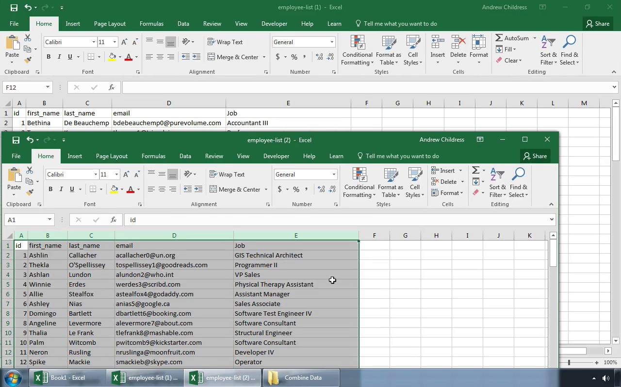
Important: The email addresses used in this tutorial are fictitious (randomly generated) and not intended to represent any real email addresses.
Read on to see written instructions. As always, Excel has multiple ways to accomplish this task, and how you’re working with your data will drive which approach is the best.
1. How to Move & Copy Sheets (Simplest Method)
The easiest method to merge Excel spreadsheets is to simply take the entire sheet and copy it from one workbook to another.
To do this, start off by opening both Excel workbooks. Then, switch to the workbook that you want to copy several sheets from.
Now, hold Control (or Command on Mac) on your keyboard and click on all of the sheets that you want to copy to a separate workbook. You’ll notice that as you do this, the tabs will show as highlighted.
Now, simply right click and choose Move or Copy from the menu.


On the Move or Copy pop up window, the first thing that you’ll want to do is select the workbook that you want to move the sheets to. Choose the name of the file from the «To book» drop-down.


Also, you can choose where the sheets are placed in the new workbook in terms of sequence. The Before sheet menu controls where sequentially in the workbook the sheets will be inserted. You can always choose (move to end) and re-sequence the order the sheets later as needed.
Finally, it’s optional check the box to Create a copy, which will duplicate the sheets and create a separate copy of them in the workbook you’re moving the sheets to. Once you press OK, you’ll see that the sheets we copied are in the combined workbook.


This approach has a few downsides. If you keep working with two separate files, they aren’t «in sync.» If you make changes to the original workbook that you copied the sheets from, they won’t automatically update in the combined workbook.
2. Prepare to Use Get & Transform Data Tools to Combine Sheets
Excel has an incredibly powerful set of tools that are often called PowerQuery. Beginning with Excel 2016, this feature set was rebranded as Get & Transform Data.
As the name suggests, these are a set of tools that helps you pull data together from other workbooks and consolidate it into one workbook.


Also, this feature is exclusive to Excel for Windows. You won’t find it in the Mac versions or in the web browser edition of Microsoft’s app.
Before You Start: Check the Data
The most important part of this process is checking your data before you start combining it. The files need to have the same setup for the data structure, with the same columns. You can’t easily combine a four-column spreadsheet and a five-column spreadsheet, as Excel won’t know where to place the data.


Often, you’ll find yourself needing to combine spreadsheets when you’re downloading data from systems. In that case, it’s much easier to make sure the system you’re downloading data is configured to download data in the same columns each time.
Before I download data from a service like Google Analytics, I always make sure that I’m downloading the same report format each time. This ensures that I can easily work with and combine multiple spreadsheets together.
Whether you’re pulling data from a system like Google Analytics, MailChimp, or an ERP like SAP or Oracle that powers huge companies, the best way to save time is to ensure that you’re downloading data in a common format.
Now that we’ve checked our data, it’s time to dive into learning how to combine Excel sheets.
3. How to Combine Excel Sheets in a Folder Full of Files
A few times, I’ve had a folder full of files that I needed to put together into a single, consolidated file. When you’ve got dozens or even hundreds of files, opening them one-by-one to combine them just isn’t feasible. Learning this technique can save you dozens of hours on a single project.
Again, it’s crucial that the data is in the same format. To get started, it helps to place all of the files in the same folder so that Excel can easily watch this folder for changes.

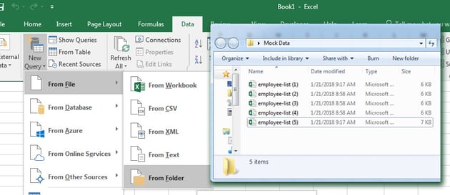

Step 1. Point Excel to the Folder of Files
On the pop-up window, you’ll want to specify a path to the folder that holds your Excel workbooks.


You can browse to that path, or simply paste in the path to the folder with your workbooks.
Step 2. Confirm the List of Files
After you show Excel where the workbooks are stored, a new window will pop up that shows the list of files you’re set to combine. Right now, you’re only seeing metadata about the files, and not the data inside of it.


This window simply shows the files that are going to be combined with our query. You’ll see the file name, the type, and the dates accessed and modified. If you’re missing a file in this list, confirm that all of the files are in the folder and retry the process.
To move on to the next step, click on Edit.
Step 3. Confirm the Combination
The next menu helps to confirm the data inside your files. Since we’ve already checked that data is the same structure in our multiple files, we can simply click OK on this step.


Step 4. How to Combine Excel Sheets With a Click
Now, a new window pops up with the list of files we’re set to combine.
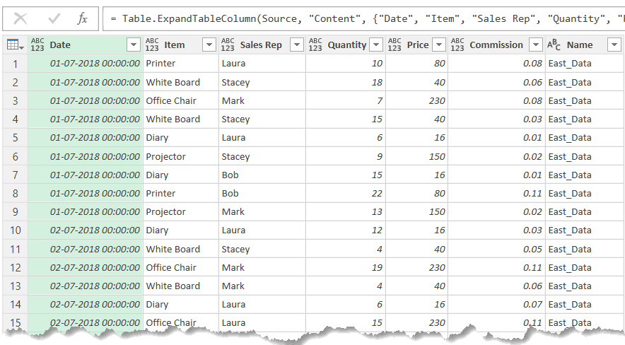
At this stage, you’re still seeing metadata about the files and now the data itself. To solve that, click on the double drop-down arrow in the upper right corner of the first column.


Voila! Now, you’ll see the actual data from inside the files combined into one place.


Scroll through the data to confirm that all of your rows are there. Notice that the only change from your original data is that the filename of each source file is in the first column.
Step 5. Close and Load the Data
Believe it or not, we’re basically finished with combining our Excel spreadsheets. The data is in the Query Editor for now, so we’ll need to «send it back» to regular Excel so that we can work with it.
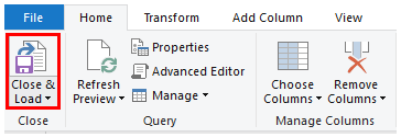
Click on Close & Load in the upper right corner. You’ll see the finished data in a regular Excel spreadsheet, ready to review and work with.


Imagine using this feature to roll up multiple files from different members of your team. Choose a folder that you’ll each store files in, and then combine them into one cohesive file with this feature in just a few minutes.
Recap & Keep Learning
In this tutorial, you learned several techniques for how to combine Excel sheets. When you’ve got many sheets that you need to stitch together, using one of these approaches will save you time so that you can get back to the task at hand!
Check out some of the other tutorials to level up your Excel skills. Each of these tutorials will teach you a method for accomplishing tasks in less time in Microsoft Excel.
How do you merge Excel workbooks? Let me know in the comments section below whether you’ve got a preference for these methods, or a technique of your own that you use.
Did you find this post useful?

I believe that life is too short to do just one thing. In college, I studied Accounting and Finance but continue to scratch my creative itch with my work for Envato Tuts+ and other clients. By day, I enjoy my career in corporate finance, using data and analysis to make decisions.
I cover a variety of topics for Tuts+, including photo editing software like Adobe Lightroom, PowerPoint, Keynote, and more. What I enjoy most is teaching people to use software to solve everyday problems, excel in their career, and complete work efficiently. Feel free to reach out to me on my website.
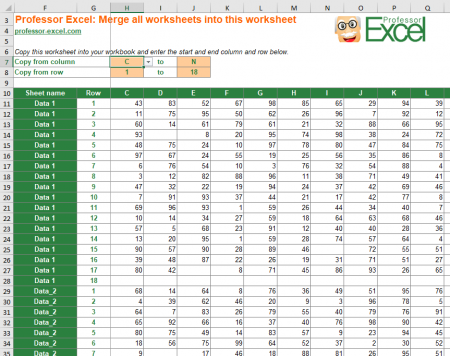
Let’s assume you have many worksheets, all in the same structure. Or they are at least in a similar structure. Now, you want to combine them into one worksheet. For example copying them underneath each other so that you can conduct lookups or insert PivotTables. In this article, you learn four methods to merge sheets in Excel.
Method 1: Copy and paste worksheets manually
In many cases it’s probably the fastest way to just copy and paste each sheet separately. That depends of course on the number of worksheets you want to combine and their structure. Some comments:
- Try to use keyboard shortcuts as much as possible. For example for selecting the complete worksheet (Ctrl + A), copying the data (Ctrl + C), navigating to your combined worksheet (Ctrl + Page Up or Page Down) and pasting the copied cells (Ctrl + V).
- Also the shortcut of pressing Ctrl on the keyboard and clicking on the little arrow in the left bottom corner of your worksheet could help. That way you jump to the first or last worksheet in your Excel workbook.
- This method is especially useful if you just have to merge sheets once. If you need to do it repeatedly (for example you get new inputs every week or month) it’s probably better to check out methods 2 to 4 below.
Method 2: Use the INDIRECT formula to merge sheets
You can use Excel formulas to combine data from all worksheets. The main formula is INDIRECT.
This method has some disadvantages, though.
- The INDIRECT formula in general is slow because it’s volatile. That means, it calculates each time Excel calculates something.
- Using a combination of INDIRECT is usually unstable and error prone.
- It takes some work to set up the INDIRECT formula.
On the other hand, it has one major advantage: If you spend effort to set it up, this method is dynamic. That means when your input updates, the merged worksheet updates as well.
Approach
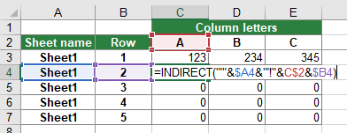
The INDIRECT formula can access any cell from a link (or better: an address) you provide. Please refer to this article to learn more about the INDIRECT formula. So you only have to provide the addresses for each cell in each worksheet you want to combine. Therefore, you should prepare a worksheet the following way (please refer to the screenshot on the right-hand side):
- Column A contains the sheet name.
- Column B contains the row number.
- Starting from Column C, you should add the column letters.
So let’s assume that you want to get the value from cell A1 of Sheet1. You would need then all the parts ‘Sheet1’, column ‘A’ and row ‘1’. Combining them in the INDIRECT formula would lead to the following formula. The formula in cell C4 is =INDIRECT(“‘”&$A4&”‘!”&C$2&$B4) .
Download
You want to save some time? We prepared a worksheet which can merge sheets automatically. What do you have to do? Download this workbook (~7 MB) and copy the only sheet into your own workbook. That’s it.
Please note the following comments.
- This method requires to enable macros (a list of all worksheets in your workbook is automatically created). When you want to save your workbook, you will be asked to switch to the XSLM file format.
- This model works for up to 50 sheets with 200 rows each (10,000 cells are prepared). If you need more, you have to extend it. The reason for this restriction is that the file is already quite large and requires some calculation performance.
Method 3: Merge sheets with a VBA Macro
You feel confident enough to use a simple VBA macro? Please insert the following code into a new VBA module. If you need assistance with VBA, please refer to this article.
Sub Merge_Sheets()
    'Insert a new worksheet
    Sheets.Add

    'Rename the new worksheet
    ActiveSheet.Name = "ProfEx_Merged_Sheet"

    'Loop through worksheets and copy the to your new worksheet
    For Each ws In Worksheets
        ws.Activate

        'Don't copy the merged sheet again
        If ws.Name <> "ProfEx_Merged_Sheet" Then
            ws.UsedRange.Select
            Selection.Copy
            Sheets("ProfEx_Merged_Sheet").Activate

            'Select the last filled cell
            ActiveSheet.Range("A1048576").Select
            Selection.End(xlUp).Select

            'For the first worksheet you don't need to go down one cell
            If ActiveCell.Address <> "$A$1" Then
                ActiveCell.Offset(1, 0).Select
            End If

            'Instead of just paste, you can also paste as link, as values etc.
            ActiveSheet.Paste

        End If

    Next
End Sub
Method 4: Combine sheets with “Professor Excel Tools”
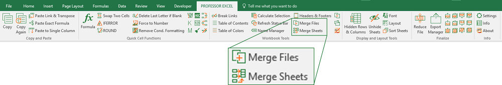
You like to use the most convenient way? Try the Excel add-in Professor Excel Tools.
- Just select all the worksheets you’d like to merge,
- click the button “Merge Sheets” and
- click on “Start”.
Alternatively, you can further refine your desired settings: Do you want to add the original sheet name in column A? No problem.
Also, define the copy & paste mode as shown in the screenshot on the right-hand side.

This function is included in our Excel Add-In ‘Professor Excel Tools’
(No sign-up, download starts directly)
(New) Method 5: Merge sheets using the Office clipboard
The first method above already dealt with copying and pasting sheets manually. There is one more trick here: Use the Excel clipboard to merge sheets. It’s actually quite simple, just follow these steps.
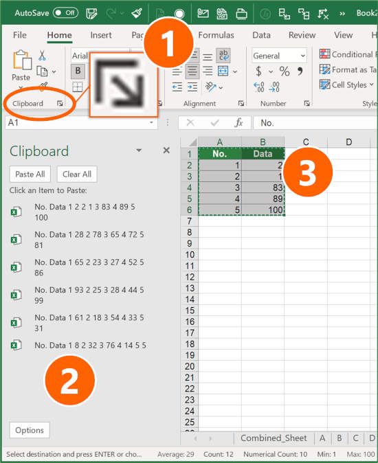
- Open the clipboard: Click on the small arrow in the right bottom corner of the Clipboard section (on the Home ribbon).
- Now you can see the clipboard.
- Next, go through each worksheet. Copy all ranges which you later want to merge on one worksheet.
- Now, you can see all your copied ranges in the clipboard.
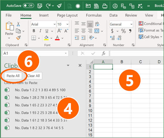
- Go to the sheet where you want to paste them underneath each other. Select the first cell.
- Click on “Paste all”
That’s it. Especially with larger files, this method could save some time compared to method number 1 above. One small disadvantage: You can further adjust the pasting method, for example using paste special to paste values only.

Henrik Schiffner is a freelance business consultant and software developer. He lives and works in Hamburg, Germany. Besides being an Excel enthusiast he loves photography and sports.
Learn everything about how to merge sheets in Excel, plus how to combine multiple Excel files into one.

Sometimes, the Microsoft Excel data you need is split across multiple sheets or even multiple files. It can be significantly more convenient to have all of this information in the same document.
You can copy and paste the cells you need in a pinch, placing them all on the same sheet. However, depending on how much data you’re working with, this might take a lot of time and effort.
Instead, we’ve rounded up some smarter ways to accomplish the same task. These methods will allow you to quickly and easily merge sheets or files in Excel.
How to Combine Excel Sheets Into One File
If you have multiple Excel files, perhaps each containing numerous sheets, that you want to combine into a single file, you can do this with the Move or Copy Sheet command. This method of merging Excel sheets has its limitations, but it’s quick and straightforward.
First, open up the sheets you want to merge into the same workbook. From there:
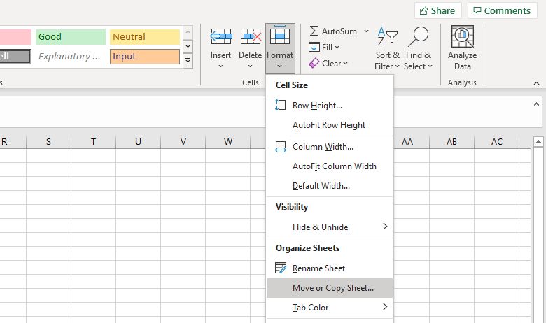
- From the top ribbon, select the Home tab.
- Within the Cells group, click Format.
- Select Move or Copy Sheet.
This opens the Move or Copy window. The To book dropdown lets you select the master spreadsheet where you want to send all of your individual sheets. Select (new book) to create a new file, or select an existing file. Use the Before sheet box to specify the order that the sheets are in (this will be blank if you’re using a new book). When ready, click OK.
Repeat this process for all the sheets that you wish to merge. To save time, you can select multiple sheets in a file by holding Ctrl as you click their tabs at the bottom.
Once done, save your new master document.
For the reverse of this, we’ve also covered how to split a large CSV into separate files.
How to Combine Excel Sheets Into One File With VBA
Rather than performing the above combination technique manually, the quicker way is to use a VBA macro. This will come in especially handy if you perform this task regularly.
First, make sure that all the files you want to combine are in the same folder on your computer. Then, create a new Excel spreadsheet that will bring them all together.
Head to the Developer tab. Within the Code section, select Visual Basic. Click Insert > Module.
For this process, we consulted ExtendOffice. Copy and paste the following code:
 Sub GetSheets()
Path = "C:FILE PATH"
Filename = Dir(Path & "*.xlsx")
  Do While Filename <> ""
  Workbooks.Open Filename:=Path & Filename, ReadOnly:=True
     For Each Sheet In ActiveWorkbook.Sheets
     Sheet.Copy After:=ThisWorkbook.Sheets(1)
  Next Sheet
     Workbooks(Filename).Close
     Filename = Dir()
  Loop
End Sub
Make sure to change the path on the second line to wherever the files are stored on your computer.
Next, click the run button (or press F5) to execute the macro. This will immediately combine all the Excel sheets into your current file. Close the Visual Basic window to return to your spreadsheet and see the result. Don’t forget to save the changes.
How to Merge Excel Data Into One Sheet
Sometimes, you might want to take more than one dataset and present it as a single sheet. This is pretty easy to accomplish in Excel, so long as you take the time to ensure that your Excel data is organized and formatted properly ahead of time.
There are two important conditions for this process to work correctly. First, the sheets you’re consolidating need to use the same layout, with identical headers and data types. Second, there can’t be any blank rows or columns.
When you’ve arranged your data to those specifications, create a new worksheet. It’s possible to run the consolidation procedure in an existing sheet where there’s already data, but it’s easier not to.
- In this new sheet, select the upper-left cell of where you want to place the consolidated data.
- Select the Data tab.
- Within the Data Tools section, click Consolidate.
- On the Function dropdown, select your desired summary function. The default is Sum, which adds values together.
- Click the up arrow button in the Reference field. If the data is in another file, use the Browse button.
- Highlight the range you wish to consolidate.
- Click Add to add the range to All references.
- Repeat step five until you’ve selected all the data that you want to consolidate.
- Check Create links to source data if you’re going to continue to update the data in other sheets and want this new sheet to reflect that. You can also select which labels are carried across with the Use labels in checkboxes.
- Finally, click OK.
Take Caution Before Merging Excel Data
Merging sheets and files in Excel can be complicated and messy. This illuminates one of the most important lessons about Microsoft Excel: it’s always good to plan ahead.
Merging different data sets after the fact is always going to cause a few headaches, especially if you’re working with large spreadsheets that have been in use for a long time. When you start working with a new workbook, it’s best to consider all possibilities of how you will use the file further down the line.
Skip to content
В статье рассматриваются различные способы объединения листов в Excel в зависимости от того, какой результат вы хотите получить:
- объединить все данные с выбранных листов,
- объединить несколько листов с различным порядком столбцов,
- объединить определённые столбцы с нескольких листов,
- объединить две таблицы Excel в одну по ключевым столбцам.
Сегодня мы займемся проблемой, с которой ежедневно сталкиваются многие пользователи Excel, — как объединить листы Excel в один без использования операций копирования и вставки. Рассмотрим два наиболее распространенных сценария: объединение числовых данных (сумма, количество, среднее и т. д.) и объединение листов ( то есть копирование данных из нескольких листов в один).
Вот что мы рассмотрим в этой статье:
- Объединение при помощи стандартного инструмента консолидации.
- Как копировать несколько листов Excel в один.
- Как объединить листы с различным порядком столбцов.
- Объединение только определённых столбцов из нескольких листов
- Слияние листов в Excel с использованием VBA
- Как объединить два листа в один по ключевым столбцам
Консолидация данных из нескольких листов на одном.
Самый быстрый способ консолидировать данные в Excel (в одной или нескольких книгах) — использовать встроенную функцию Excel Консолидация.
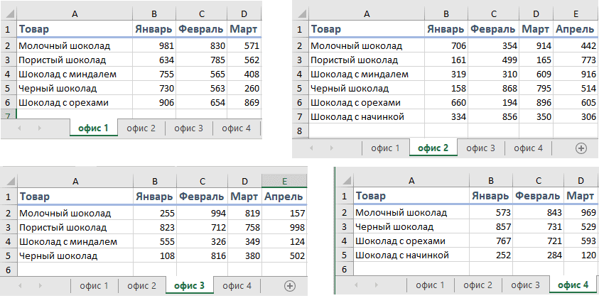
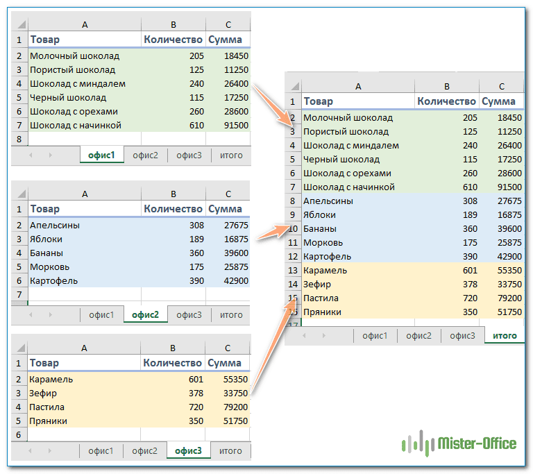
Рассмотрим следующий пример. Предположим, у вас есть несколько отчетов из региональных офисов вашей компании, и вы хотите объединить эти цифры в основной рабочий лист, чтобы у вас был один сводный отчет с итогами продаж по всем товарам.
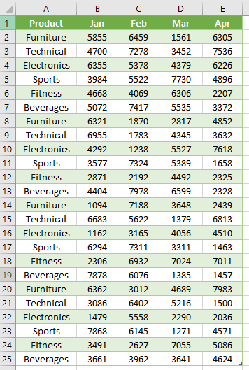
Как вы видите на скриншоте ниже, четыре объединяемых листа имеют схожую структуру данных, но разное количество строк и столбцов:
Чтобы объединить всю эту информацию на одном листе, выполните следующие действия:
- Правильно расположите исходные данные. Чтобы функция консолидации Excel работала правильно, убедитесь, что:
- Каждый диапазон (набор данных), который вы хотите объединить, находится на отдельном листе. Не помещайте данные на лист, куда вы планируете выводить консолидированные данные.
- Каждый лист имеет одинаковый макет, и каждый столбец имеет заголовок и содержит похожие данные.
- Ни в одном списке нет пустых строк или столбцов.
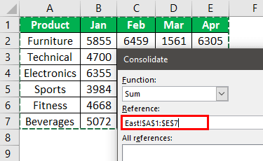
- Запустите инструмент «Консолидация». На новом листе, где вы планируете поместить результаты, щелкните верхнюю левую ячейку, начиная с которой должны отображаться консолидированные данные, затем на ленте перейдите на вкладку «Данные» и нажмите кнопку «Консолидация».
Совет. Желательно объединить данные в пустой лист. Если на вашем основном листе уже есть данные, убедитесь, что имеется достаточно места (пустые строки и столбцы) для записи результатов.
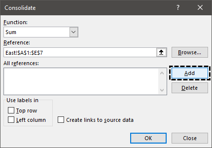
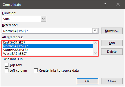
- Настройте параметры консолидации. Появляется диалоговое окно «Консолидация», и вы делаете следующее:
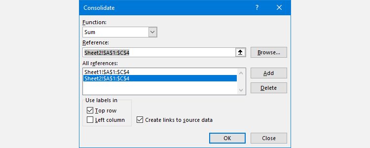
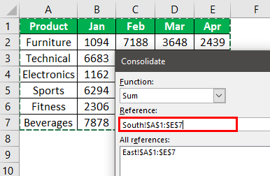
- В поле «Функция» выберите одну из функций, которую вы хотите использовать для консолидации данных (количество, среднее, максимальное, минимальное и т. д.). В этом примере мы выбираем Сумма.
- В справочном окне, нажав в поле Ссылка на значок
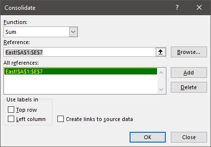
 , выберите диапазон на первом листе. Затем нажмите кнопку «Добавить», чтобы присоединить его к списку диапазонов. Повторите этот шаг для всех листов, которые вы хотите объединить.
Если один или несколько листов находятся в другой книге, используйте кнопку «Обзор», чтобы найти эту книгу и использовать ее.
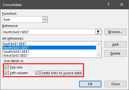
- Настройте параметры обновления. В том же диалоговом окне Консолидация выберите любой из следующих параметров:
- Установите флажки «Подписи верхней строки» и / или «Значения левого столбца» в разделе «Использовать в качестве имён», если вы хотите, чтобы заголовки строк и / или столбцов исходных диапазонов были также скопированы.
- Установите флажок «Создать связи с исходными данными», если нужно, чтобы консолидированные данные обновлялись автоматически при изменении исходных таблиц. В этом случае Excel создаст ссылки на ваши исходные листы, а также схему, как на следующем скриншоте:
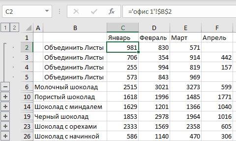
Если вы развернете какую-либо группу (щелкнув значок плюса), а затем установите курсор на ячейку с определенным значением, в строке формул отобразится ссылка на исходные данные.
Если флажок не устанавливать, то вы получаете просто таблицу с итоговыми цифрами без всяких формул и ссылок:

Как видите, функция консолидации Excel очень полезна для сбора данных. Однако у нее есть несколько ограничений. В частности, он работает только для числовых значений и всегда обрабатывает эти числа тем или иным образом (сумма, количество, среднее и т. д.). Исходные цифры вы здесь не увидите.
Если вы хотите объединить листы в Excel, просто скопировав и объединив их содержимое, вариант консолидации не подходит. Чтобы объединить всего парочку из них, создав как бы единый массив данных, то вам из стандартных возможностей Excel не подойдёт ничего, кроме старого доброго копирования / вставки.
Но если вам предстоит таким образом обработать десятки листов, ошибки при этом будут практически неизбежны. Да и затраты времени весьма значительны.
Поэтому для подобных задач рекомендую использовать один из перечисленных далее нестандартных методов для автоматизации слияния.
Как скопировать несколько листов Excel в один.
Как мы уже убедились, встроенная функция консолидации умеет суммировать данные из разных листов, но не может объединять их путем копирования данных на какой-то итоговый лист. Для этого вы можете использовать один из инструментов слияния и комбинирования, включенных в надстройку Ultimate Suite для Excel.
Для начала давайте будем исходить из следующих условий:
- Структура таблиц и порядок столбцов на всех листах одинаковы.
- Количество строк везде разное.
- Листы могут в будущем добавляться или удаляться.
Итак, у вас есть несколько таблиц, содержащих информацию о различных товарах, и теперь вам нужно объединить эти таблицы в одну итоговую, например так, как на рисунке ниже:
Три простых шага — это все, что нужно, чтобы объединить выбранные листы в один.
1. Запустите мастер копирования листов.
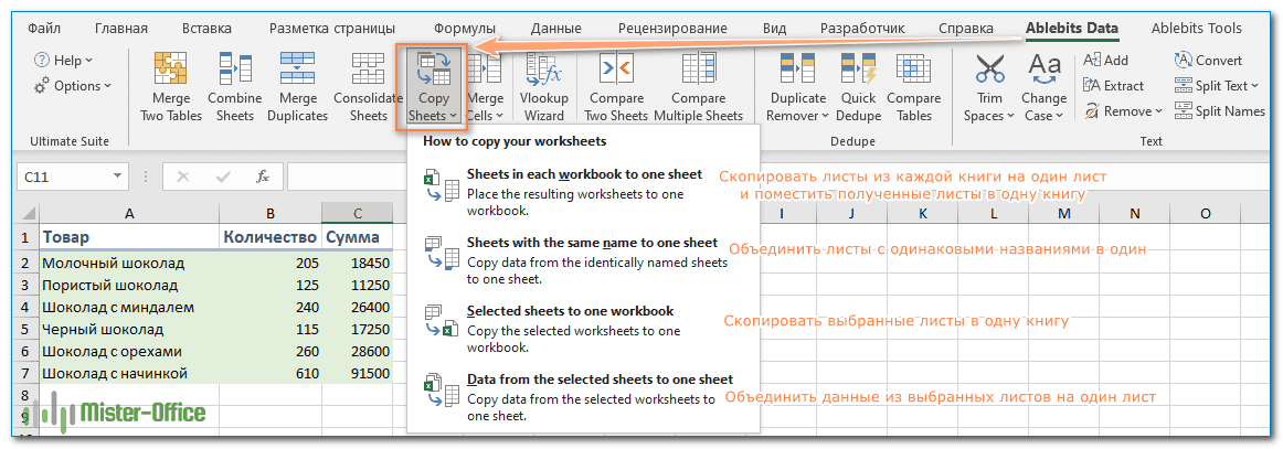
На ленте перейдите на вкладку AblebitsData, нажмите «Копировать листы (Copy Sheets)» и выберите один из следующих вариантов:
- Скопировать листы из каждой книги на один лист и поместить полученные листы в одну книгу.
- Объединить листы с одинаковыми названиями в один.
- Скопировать выбранные в одну книгу.
- Объединить данные из выбранных листов на один лист.
Поскольку мы хотим объединить несколько листов путем копирования их данных, то выбираем последний вариант:
1. Выберите листы и, при необходимости, диапазоны для объединения.
Мастер копирования листов отображает список всех имеющихся листов во всех открытых книгах. Выберите те из них, которые хотите объединить, и нажмите « Далее».
Если вы не хотите копировать все содержимое определенного рабочего листа, используйте специальный значок, чтобы выбрать нужный диапазон, как показано на скриншоте ниже.
В этом примере мы объединяем первые три листа нашей книги:
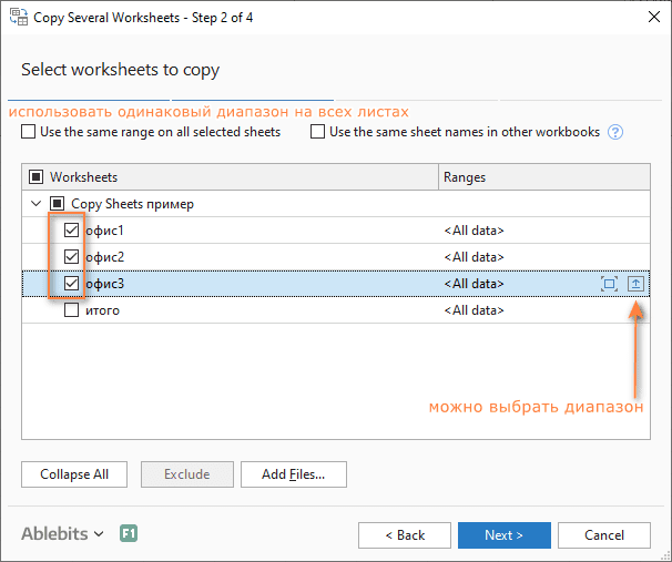
Совет. Если рабочие листы, которые вы хотите объединить, находятся в другой книге, которая в данный момент закрыта, нажмите кнопку «Добавить файлы …» , чтобы найти и открыть эту книгу.
2. Выберите, каким образом произвести объединение.
На этом этапе вы должны настроить дополнительные параметры, чтобы ваша информация была объединена именно так, как вы хотите.
Как вставить :
- Вставить все – скопировать все данные (значения и формулы). В большинстве случаев это правильный выбор.
- Вставлять только значения – если вы не хотите, чтобы переносились формулы, выберите этот параметр.
- Создать ссылки на исходные данные – это добавит формулы, связывающие итоговые ячейки с исходными. Выберите этот параметр, если вы хотите, чтобы результат объединения обновлялся автоматически при изменении исходных файлов. Это работает аналогично параметру «Создать ссылки на исходные данные» в стандартном инструменте консолидации в Excel.
Как расположить :
- Разместите скопированные диапазоны один под другим – то есть вертикально.
- Расположить скопированные диапазоны рядом – то есть по горизонтали.
Как скопировать :
- Сохранить форматирование – понятно и очень удобно.
- Разделить скопированные диапазоны пустой строкой – выберите этот вариант, если вы хотите добавить пустую строку между сведениями, скопированными из разных листов. Так вы сможете отделить их друг от друга, если это необходимо.
- Скопировать таблицы вместе с их заголовками. Установите этот флажок, если хотите, чтобы заголовки исходных таблиц были включены в итоговый лист.
На скриншоте ниже показаны настройки по умолчанию, которые нам подходят:

Нажмите кнопку «Копировать (Copy)», и у вас будет содержимое трех разных листов, объединенное в один итоговый, как показано в начале этого примера.
Быть может, вы скажете, что подобную операцию можно произвести путем обычного копирования и вставки. Но если у вас будет десяток или более листов и хотя бы несколько сотен строк на каждом из них, то это будет весьма трудоемкой операцией, которая займет довольно много времени. Да и ошибки вполне вероятны. Использование надстройки сэкономит вам много времени и избавит от проблем.
Как объединить листы Excel с различным порядком столбцов.
Когда вы имеете дело с файлами, созданными разными пользователями, порядок столбцов в них часто отличается. Как же их объединить? Будете ли вы копировать вручную или перемещать столбцы, чтобы упорядочить их в каждой книге? Это совсем не выход.
Используем инструмент объединения листов Combine Sheets.
Запускаем надстройку через меню Ablebits Data – Combine Sheets.

Выбираем и отмечаем галочками те листы, данные с которых мы хотим объединить. Затем программа анализирует их и предлагает нам список найденных столбцов с указанием того, сколько раз столбец с подобным названием был обнаружен.

Вы должны указать те столбцы, данные из которых вы хотели бы объединить. Можете выбрать их все, можете – только самые важные.
Затем определяем, как нужно вставить собранные данные: целиком с формулами или только значения, либо сформировать ссылки на источники, чтобы обеспечить постоянное обновление и актуальность информации в случае внесения изменений в исходные таблицы.

Также можно указать, что необходимо сохранить исходное форматирование, если оно уникально в каждой таблице. Так вам, кстати, будет проще определить, откуда появились сведения в общем массиве, какая таблица является их источником.
И данные будут идеально скомпонованы по заголовкам столбцов:
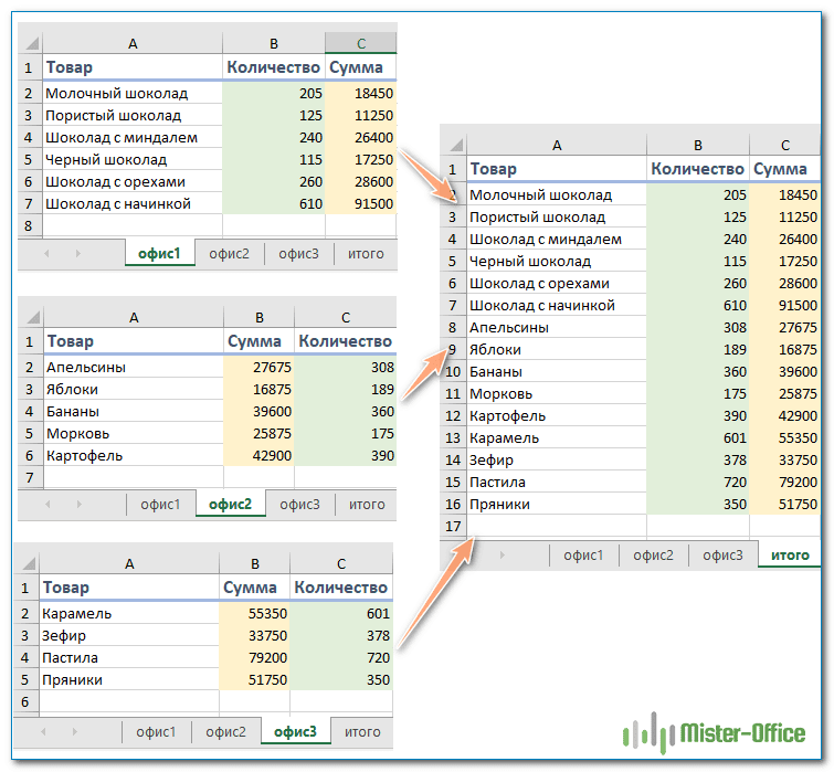
Мы получили своего рода сводную таблицу с необходимой информацией.
Объединение определенных столбцов из нескольких листов.
А вот, как мне кажется, наиболее часто встречающаяся ситуация:
- у вас действительно большие листы с множеством разных столбцов,
- столбцы расположены на каждом из них по-разному, в произвольном порядке,
- необходимо объединить только самые важные из них в итоговую таблицу.
Запустите мастер объединения листов, как мы это делали в предыдущем примере, укажите нужные, а затем выберите соответствующие столбцы. Да, это так просто!

Все дальнейшие шаги мы уже описывали выше. В результате в итоговую таблицу попадают только данные из выбранных вами столбцов:

Эти примеры продемонстрировали только несколько инструментов слияния данных, но это еще не все! Немного поэкспериментировав, вы увидите, насколько полезны и удобны все функции, включенные в пакет.
Полнофункциональная ознакомительная версия Ultimate Suite доступна для загрузки в по этой ссылке.
Слияние листов в Excel с помощью кода VBA
Если вы опытный пользователь Excel и чувствуете себя комфортно с макросами и VBA, вы можете объединить несколько листов Excel в один, используя какой-нибудь сценарий.
Для этого на вкладке Разработчик (Developer) нажмите кнопку Visual Basic или воспользуйтесь сочетанием клавиш Alt+F11. В открывшемся окне добавьте новый модуль через меню Insert — Module и скопируйте туда текст вот такого макроса:
Sub CopyDataWithHeaders()
    Dim sh As Worksheet
    Dim DestSh As Worksheet
    Dim Last As Long
    Dim shLast As Long
    Dim CopyRng As Range
    Dim StartRow As Long

    With Application
        .ScreenUpdating = False
        .EnableEvents = False
    End With

    'Delete the sheet "RDBMergeSheet" if it exist
    Application.DisplayAlerts = False
    On Error Resume Next
    ActiveWorkbook.Worksheets("RDBMergeSheet").Delete
    On Error GoTo 0
    Application.DisplayAlerts = True

    'Add a worksheet with the name "RDBMergeSheet"
    Set DestSh = ActiveWorkbook.Worksheets.Add
    DestSh.Name = "RDBMergeSheet"

    'Fill in the start row
    StartRow = 2

    'loop through all worksheets and copy the data to the DestSh
    For Each sh In ActiveWorkbook.Worksheets
        If sh.Name <> DestSh.Name Then

'Copy header row, change the range if you use more columns
If WorksheetFunction.CountA(DestSh.UsedRange) = 0 Then
  sh.Range("A1:Z1").Copy DestSh.Range("A1")
End If

            'Find the last row with data on the DestSh and sh
            Last = LastRow(DestSh)
            shLast = LastRow(sh)

            'If sh is not empty and if the last row >= StartRow copy the CopyRng
            If shLast > 0 And shLast >= StartRow Then

                'Set the range that you want to copy
                Set CopyRng = sh.Range(sh.Rows(StartRow), sh.Rows(shLast))

                'Test if there enough rows in the DestSh to copy all the data
                If Last + CopyRng.Rows.Count > DestSh.Rows.Count Then
                    MsgBox "There are not enough rows in the Destsh"
                    GoTo ExitTheSub
                End If

                'This example copies values/formats, if you only want to copy the
                'values or want to copy everything look below example 1 on this page
                CopyRng.Copy
                With DestSh.Cells(Last + 1, "A")
                    .PasteSpecial xlPasteValues
                    .PasteSpecial xlPasteFormats
                    Application.CutCopyMode = False
                End With

            End If

        End If
    Next

ExitTheSub:

    Application.Goto DestSh.Cells(1)

    'AutoFit the column width in the DestSh sheet
    DestSh.Columns.AutoFit

    With Application
        .ScreenUpdating = True
        .EnableEvents = True
    End With
End Sub

Function LastRow(sh As Worksheet)
    On Error Resume Next
    LastRow = sh.Cells.Find(What:="*", _
                            After:=sh.Range("A1"), _
                            Lookat:=xlPart, _
                            LookIn:=xlFormulas, _
                            SearchOrder:=xlByRows, _
                            SearchDirection:=xlPrevious, _
                            MatchCase:=False).Row
    On Error GoTo 0
End Function


Function LastCol(sh As Worksheet)
    On Error Resume Next
    LastCol = sh.Cells.Find(What:="*", _
                            After:=sh.Range("A1"), _
                            Lookat:=xlPart, _
                            LookIn:=xlFormulas, _
                            SearchOrder:=xlByColumns, _
                            SearchDirection:=xlPrevious, _
                            MatchCase:=False).Column
    On Error GoTo 0
End Function
Имейте в виду, что для правильной работы кода VBA все исходные листы должны иметь одинаковую структуру, одинаковые заголовки столбцов и одинаковый порядок столбцов.
В этой функции выполняется копирование данных со всех листов начиная со строки 2 и до последней строки с данными. Если шапка в ваших таблицах занимает две или более строки, то измените этот код, поставив вместо 2 цифры 3, 4 и т.д.:
    'Fill in the start row
    StartRow = 2
При запуске функция добавит в вашу книгу рабочий лист с именем RDBMergeSheet и скопирует на него ячейки из каждого листа в книге. Каждый раз, когда вы запускаете макрос, он
сначала удаляет итоговый рабочий лист с именем RDBMergeSheet, если он существует, а затем добавляет новый в книгу. Это гарантирует, что данные всегда будут актуальными после запуска кода. При этом формат объединяемых ячеек также копируется.
Ещё несколько интересных примеров кода VBA для объединения листов вашей рабочей книги вы можете найти по этой ссылке.
Как объединить два листа Excel в один по ключевому столбцу
Если вы ищете быстрый способ сопоставить и объединить данные из двух листов, вы можете либо использовать функцию Excel ВПР, либо воспользоваться мастером объединения таблиц Merge Two Tables.
Последний представляет собой удобный визуальный инструмент, который позволяет сравнивать две таблицы Excel по общему столбцу (столбцам) и извлекать совпадающие данные из справочной таблицы. На скриншоте ниже показан один из возможных результатов.

Более подробно его работа рассмотрена в этой статье.
Мастер объединения двух таблиц также включен в Ultimate Suite for Excel, как и множество других полезных функций.
Вот как вы можете объединить листы в Excel. Я надеюсь, что вы найдете информацию в этом коротком руководстве полезной. Если у вас есть вопросы, не стесняйтесь оставлять их в комментариях.
 Быстрое удаление пустых столбцов в Excel — В этом руководстве вы узнаете, как можно легко удалить пустые столбцы в Excel с помощью макроса, формулы и даже простым нажатием кнопки. Как бы банально это ни звучало, удаление пустых…
  Как быстро объединить несколько файлов Excel — Мы рассмотрим три способа объединения файлов Excel в один: путем копирования листов, запуска макроса VBA и использования инструмента «Копировать рабочие листы» из надстройки Ultimate Suite. Намного проще обрабатывать данные в…
  Как работать с мастером формул даты и времени — Работа со значениями, связанными со временем, требует глубокого понимания того, как функции ДАТА, РАЗНДАТ и ВРЕМЯ работают в Excel. Эта надстройка позволяет быстро выполнять вычисления даты и времени и без особых…
  Как найти и выделить уникальные значения в столбце — В статье описаны наиболее эффективные способы поиска, фильтрации и выделения уникальных значений в Excel. Ранее мы рассмотрели различные способы подсчета уникальных значений в Excel. Но иногда вам может понадобиться только просмотреть уникальные…
  Как получить список уникальных значений — В статье описано, как получить список уникальных значений в столбце с помощью формулы и как настроить эту формулу для различных наборов данных. Вы также узнаете, как быстро получить отдельный список с…
  Как объединить две или несколько таблиц в Excel — В этом руководстве вы найдете некоторые приемы объединения таблиц Excel путем сопоставления данных в одном или нескольких столбцах. Как часто при анализе в Excel вся необходимая информация собирается на одном…
Содержание
- Merge Excel Files: How to Combine Workbooks into One File
- Summary
- Method 1: Copy the cell ranges
- Method 2: Manually copy worksheets
- Method 3: Use the INDIRECT formula
- Method 4: Merge files with a simple VBA macro
- Method 5: Automatically merge workbooks
- Method 6: Use the Get & Transform tools (PowerQuery)
- Next step: Merge multiple worksheets to one combined sheet
- 39 comments
Merge Excel Files: How to Combine Workbooks into One File

You have several Excel workbooks and you want to merge them into one file? This could be a troublesome and long process. But there are 6 different methods of how to merge existing workbooks and worksheets into one file. Depending on the size and number of workbooks, at least one of these methods should be helpful for you. Let’s take a look at them.
Summary
If you want to merge just a small amount of files, go with methods 1 or method 2 below. For anything else, please take a look at the methods 4 to 6: Either use a VBA macro, conveniently use an Excel-add-in or use PowerQuery (PowerQuery only possible if the sheets to merge have exactly the same structure).
Method 1: Copy the cell ranges
The obvious method: Select the source cell range, copy and paste them into your main workbook. The disadvantage: This method is very troublesome if you have to deal with several worksheets or cell ranges. On the other hand: For just a few ranges it’s probably the fastest way.
Method 2: Manually copy worksheets
The next method is to copy or move one or several Excel sheets manually to another file. Therefore, open both Excel workbooks: The file containing the worksheets which you want to merge (the source workbook) and the new one, which should comprise all the worksheets from the separate files.
- Select the worksheets in your source workbooks which you want to copy. If there are several sheets within one file, hold the Ctrl key and click on each sheet tab. Alternatively, go to the first worksheet you want to copy, hold the Shift key and click on the last worksheet. That way, all worksheets in between will be selected as well.
- Once all worksheets are selected, right click on any of the selected worksheets.
- Click on “Move or Copy”.
- Select the target workbook.
- Set the tick at “Create a copy”. That way, the original worksheets remain in the original workbook and a copy will be created.
- Confirm with OK.
 and click on each sheet tab. Alternatively, go to the first worksheet you want to copy, hold the Shift key
  and click on the last worksheet. That way, all worksheets in between will be selected as well.
One small tip at this point: You can just drag and drop worksheets from one to another Excel file. Even better: If you press and hold the Ctrl-Key when you drag and drop the worksheets, you create copies.
Do you want to boost your productivity in Excel?
Get the Professor Excel ribbon!

Add more than 120 great features to Excel!
Method 3: Use the INDIRECT formula
The next method comes with some disadvantages and is a little bit more complicated. It works, if your files are in a systematic file order and just want to import some certain values. You build your file and cell reference with the INDIRECT formula. That way, the original files remain and the INDIRECT formula only looks up the values within these files. If you delete the files, you’ll receive #REF! errors.
Let’s take a closer look at how to build the formula. The INDIRECT formula has only one argument: The link to another cell which can also be located within another workbook.
- Copy the first source cell.
- Paste it into your main file using paste special (Ctrl + Alt + v ). Instead of pasting it normally, click on “Link” in the bottom left corner of the Paste Special window. That way, you extract the complete path. In our case, we have the following link:
=[160615_Examples.xlsm]Thousands!$C$4 - Now we wrap the INDIRECT formula around this path. Furthermore, we separate it into file name, sheet name and cell reference. That way, we can later on just change one of these references, for instance for different versions of the same file. The complete formula looks like this (please also see the image above):
=INDIRECT(“‘”&$A3&$B3&”‘!”&D$2&$C3)
 + v
+ v  ). Instead of pasting it normally, click on “Link” in the bottom left corner of the Paste Special window. That way, you extract the complete path. In our case, we have the following link:
Important – please note: This function only works if the source workbooks are open.
Method 4: Merge files with a simple VBA macro
You are not afraid of using a simple VBA macro? Then let’s insert a new VBA module:
- Go to the Developer ribbon. If you can’t see the Developer ribbon, right click on any ribbon and then click on “Customize the Ribbon…”. On the right hand side, set the tick at “Developer”.
- Click on Visual Basic on the left side of the Developer ribbon.
- Right click on your workbook name and click on Insert –> Module.
- Copy and paste the following code into the new VBA module. Position the cursor within the code and click start (the green triangle) on the top. That’s it!
Method 5: Automatically merge workbooks
The fifth way is probably most convenient:
Click on “Merge Files” on the Professor Excel ribbon.
Now select all the files and worksheets you want to merge and start with “OK”.
This procedure works well also for many files at the same time and is self-explanatory. Even better: Besides XLSX files, you can also combine XLS, XLSB, XLSM, CSV, TXT and ODS files.
To do that you need a third party add-in, for example our popular “Professor Excel Tools” (click here to start the download).
Here is the whole process in detail:
 Just click on “Merge Files” on the Professor Excel ribbon, select your files and click on OK.
![]()
![]()
![]()
The current version of Excel 365 offers the “Get & Transform” tools to import data. These functions are very powerful and are supposed to replace the old “Text Import Wizard”. However, they have one useful feature: Import a complete folder of documents.
The requirements: The workbooks and worksheets you want to import have to be in the same format.
Please follow these steps for importing a complete folder of Excel files.
- Create a folder with all the documents you want to import.
- Usually it’s the fastest to just copy the folder path directly from the Windows Explorer. You still have the change to later-on select the folder, though.
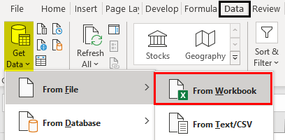
- Within Excel, go to the Data ribbon and click on “Get Data”, “From File” and then on “From Folder”.
- Paste the previously copied path or select it via the “Browse” function. Continue with “OK”.
- If all files are shown in the following window, either click on “Combine” (and then on “Combine & Load To”) or on “Edit”. If you click on “Edit”, you can still filter the list and only import a selection of the files in the list. Recommendation: Put only the necessary files into your import folder from the beginning so that you don’t have to navigate through the complex “Edit” process.
- Next, Excel shows an example of the data based on the first file. If everything seems fine, click on OK. If your files have several sheets, just select the one you want to import, in this example “Sheet1”. Click on “OK”.
- That’s it, Excel now imports the data and inserts a new column containing the file name.
For more information about the Get & Transform tools please refer to this article.
Next step: Merge multiple worksheets to one combined sheet
After you have combined many Excel workbooks into one file, usually the next step is this: Merge all the imported sheets into one worksheet.
Because this is a whole different topic by itself, please refer to this article.
Henrik Schiffner is a freelance business consultant and software developer. He lives and works in Hamburg, Germany. Besides being an Excel enthusiast he loves photography and sports.
I want a routine to compare and merge some workbook into one or only merge some workbooks into one. I don’t want a only copy a sheet, no…. I want to MERGE copies of one workbook into one.
I hope you can help me
Hi. I used method 4 to merge numerous excel files into one workbook.
After each file it gives me a message that says “The name ‘NvsInstanceHook’ already exists. Click Yes to use that version of the name or click No to rename the version of ‘NvsInstanceHook’ you’re moving or copying”
I click yes. Then it asks me if I want to save or not save the file. I click not save,
How do I get the script to automate answering both those prompts so I don’t need to manually select?
Also, how do I save this script so I can keep using it over and over again?
I used the VBA method which worked like a charm except I had to click “save” after every file was processed. Is there any way to include that in the module?
Hi Jacqui,
Please replace this line:
Application.DisplayAlerts = False
sourceWorkbook.Close
Application.DisplayAlerts = True
This should avoid the error messages. But please make sure that your work is saved…
“Method 5: Automatically merge workbooks
The third way is probably most convenient:”
Is that a “Monty Python & the Holy Grail” reference? 😀
Haven’t seen it actually. But I corrected the mistake… it’s the fifth way 😉
Method 4 has made my life very easy……………………..
Hi
I tried method 4 (VBA) and it works fine for a simple merge.
But what I want is to update the merge task withou duplicate sheets.
Explaining:
I have three large files updating in a daily basis (each one with one sheet). Then i need to merge all of them into one evaryday.
Using your method 4 for second time, it duplicates sheets, instead of replacing the existing sheets.
So, it would be nice if you provide the changes needed in your code to do the update and, if possible, to execute automatically every 24 hours.
Thank You very much for your time
JT
i want to combine a specific sheet from the source files to a work book. Not all the work sheets in the source files.Suppose three product files , (product1 , product2 and product3) all the files has many sheets like sales,employees, expenses and so on. But i need only sales sheets from all the 3 product files into one work book (not in one work sheet)
Hi Hari,
I’m working on an advanced merge function for my add-in. But it’ll take some time.
Best regards,
Henrik
Hi
when i used vba code it worked fine but i want all the data to merged in one single worksheet instead of seperate worksheets in one workbook.
Hi VVS,
Please check out this article: https://professor-excel.com/merge-sheets/. After merging the data into one workbook (on separate sheets), you can copy them underneath each other on one single worksheet.
Best regards,
Henrik
Hi Henrik,
Instead of running the code twice is there any chance that merging the data from different works books into one single workbook on one tym running the vba code .
What if you aren’t merging workbooks (.xlsx), but other data files saves as .csv, or .txt, or .dat .. can the VBA script handle those?
Hi Jo,
Probably it’ll work as well. Just give it a try…
Henrik
Thanks very much for your code, I tried it, it works but I have this error message: Run-time error ‘1004’ Method ‘Copy’ of object ‘Worksheet’ failed, could you please help me on this.
Hi Henrik, the code corked fine. now ,i want to delete the header rows in the merge file when it is executed and should display only final header row at the top but not all the header rows.
I have multiple workbooks with multiple worksheets (same columns for all workbooks, but different columns within each workbook ie. both book1 and book2 have sheet1 and sheet2, or more). Your code adds ALL sheets one after another, so I end up having 4 tabs in the output. Can you tweak it so sheet1 from book1 and book2 are merged in one new sheet, and sheet2 from book1 and book2 are merged in another sheet (2 sheets 1 workbook in the output)? Thanks!
thank you very much for the VBA code.
Could you please help me a bit related to that code?
I should copy only the 2nd, 3rd and 4th sheets from each excel workbook into a separate one. How should I change the code to be able to avoid the remaining tabs?
Thank you,
Renato
I seriously love you for posting #4 (with the adjustment in your comment reply. Instead of requesting more customization I’ll tell you a story. I’ve been on a self-directed crash-course in VBA since stepping into an analyst role two weeks ago, tasked with (among other things) collecting and tracking responses for procedural non-compliance from a few hundred field units. Old method: field offices were sent a 32-column data export and attempted to copy/paste the rows which apply to their office into a separate “Response Form” (aka a Word doc) along with additional identifying info and investigation/action details. The analyst tracked responses by highlighting lines on a pivot table, which was challenging because few field units could successfully copy/paste 32 cells or provide all requested info or type a Subject line that distinguished one response from 100 others. My method: Turned the Word Doc into a 32-column worksheet, merged it with the data export, added a Double-Click event function so *anyone* can fully populate their response form directly from the data export tab; gave the form a 1-click “Submit” function which references identifying data (via their double-click event) to rename the worksheet which then duplicates and emails itself to me with a subject line that also references identifying data; found Outlook VBA that extracts all attachments from the folder which their responses (with those uniform and predictable subject lines) are filtered to, to an Import-folder on my desktop; and a tracker column on my master data export which matches identifying info from the response sheets as I import them into the tracking worksheet. The ONLY thing missing has been a convenient way to batch-import those attachments into the tracker without requiring an Add-In (miles of red tape to get one approved). I knew it could be done but was unable to find an answer for the past two weeks before stumbling onto this post. You’re a God-send at the end of a 13-hour day. Thank you.
Источник
I recently got a question from a reader about combining multiple worksheets in the same workbook into one single worksheet.
I asked him to use Power Query to combine different sheets, but then I realized that for someone new to Power Query, doing this can be tough.
So I decided to write this tutorial and show the exact steps to combine multiple sheets into one single table using Power Query.
Below a video where I show how to combine data from multiple sheets/tables using Power Query:
Below are written instructions on how to combine multiple sheets (in case you prefer written text over video).
Note: Power Query can be used as an add-in in Excel 2010 and 2013, and is an inbuilt feature from Excel 2016 onwards. Based on your version, some images may look different (image captures used in this tutorial are from Excel 2016).

Combine Data from Multiple Worksheets Using Power Query
When combining data from different sheets using Power Query, it’s required to have the data in an Excel Table (or at least in named ranges). If the data is not in an Excel Table, the method shown here would not work.
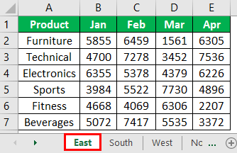
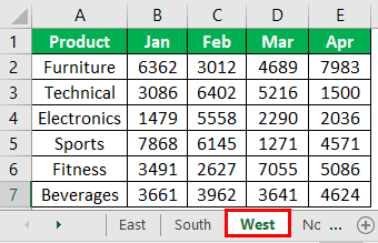
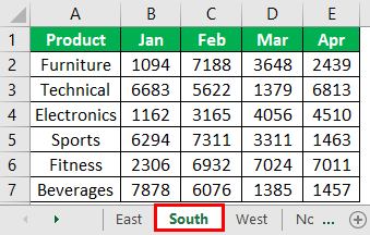
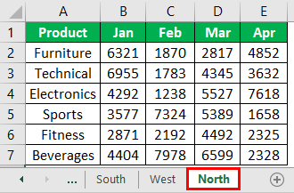
Suppose you have four different sheets – East, West, North, and South.
Each of these worksheets has the data in an Excel Table, and the structure of the table is consistent (i.e., the headers are same).

Click here to download the data and follow along.
This kind of data is extremely easy to combine using Power Query (which works really well with data in Excel Table).
For this technique to work best, it’s better to have names for your Excel Tables (work without it too, but it’s easier to use when the tables are named).
I have given the tables the following names: East_Data, West_Data, North_Data, and South_Data.
Here are the steps to combine multiple worksheets with Excel Tables using Power Query:
- Go to the Data tab.

- In the Get & Transform Data group, click on the ‘Get Data’ option.

- Go the ‘From Other Sources’ option.
- Click the ‘Blank Query’ option. This will open the Power Query editor.

- In the Query editor, type the following formula in the formula bar: =Excel.CurrentWorkbook(). Note that the Power Query formulas are case sensitive, so you need to use the exact formula as mentioned (else you will get an error).

- Hit the Enter key. This will show you all the table names in the entire workbook (it will also show you the named ranges and/or connections in case it exists in the workbook).

- [Optional Step] In this example, I want to combine all the tables. If you want to combine specific Excel Tables only, then you can click the drop-down icon in the name header and select the ones you want to combine. Similarly, if you have named ranges or connections, and you only want to combine tables, you can remove those named ranges as well.
- In the Content header cell, click on the double pointed arrow.
- Select the columns that you want to combine. If you want to combine all columns, make sure (Select All Columns) is checked.
- Uncheck the ‘Use original column name as prefix’ option.

- Click OK.


The above steps would combine the data from all the worksheets into one single table.
If you look closely, you’ll find the last column (rightmost) has the name of the Excel tables (East_Data, West_Data, North_Data, and South_Data). This is an identifier that tells us which record came from which Excel Table. This is also the reason I said it’s better to have descriptive names for the Excel tables.
Here are a few modifications you can do to the combined data in Power Query itself:
- Drag and place the Name column to the beginning.
- Remove the “_Data” from the name column (so you’re left with East, West, North, and South in the name column). To do this, right-click on the Name header and click on Replace Values. In the Replace Values dialog box, replace _Data with a blank.
- Change the Data column to show only dates (and not the time). To do this, click the Date column header, go to the ‘Transform’ tab and change the Data type to Date.
- Rename the Query to ConsolidatedData.
Now that you have the combined data from all the worksheets in Power Query, you can load it in Excel – as a new table in a new worksheet.
To do this. follow the below steps:
- Click the ‘File’ tab.
- Click on Close and Load To.

- In the Import Data dialog box, select Table and New worksheet options.

- Click Ok.


The above steps would combine data from all the worksheets and give you that combined data in a new worksheet.
One Issue You Must Resolve when Using This Method
In case you have used the above method to combine all the tables in the workbook, you’re likely to face an issue.
See the number of rows of the combined data – 1304 (which is right).

Now, if I refresh the query, the number of rows changes to 2607. Refresh again and it will change to 3910.

Here is the problem.
Every time you refresh the query, it adds all the records in the original data to the combined data.
Note: You’ll face this issue only if you have used Power Query to combine ALL THE EXCEL TABLES in the workbook. In case you selected specific tables to be combined, you’ll not face this issue.
Let’s understand the cause of this problem and how to correct this.
When you refresh a query, it goes back and follows all the steps that we took to combine the data.
In the step where we used the formula =Excel.CurrentWorkbook(), it gave us a list of all the tables. This worked fine the first time as there were only four tables.
But when you refresh, there are five tables in the workbook – including the new table that Power Query inserted where we have the combined data.
So every time you refresh the query, apart from the four Excel Tables that we want to combine, it also adds the existing query table to the resulting data.
This is called recursion.
Here is how to solve this issue.
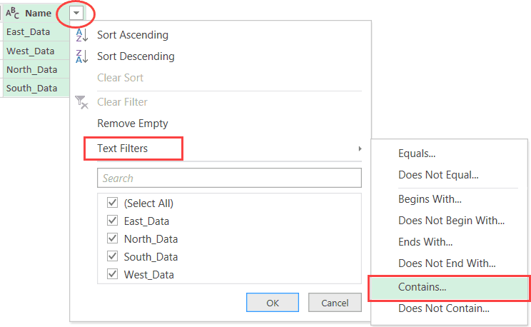
Once you insert =Excel.CurrentWorkbook() in the Power Query formula bar and hit enter, you get a list of Excel Tables. To make sure you only get to combine the tables from the worksheet, you need to somehow filter only these tables that you want to combine and remove everything else.
Here are the steps to make sure you only have the required tables:
- Click the drop-down and hover the cursor on Text Filters.
- Click on the Contains option.

- In the Filter Rows dialog box, enter _Data in the field next to the ‘contains’ option.

- Click OK.

You may not see any change in the data, but doing this will prevent the resulting table from being added over again when the query is refreshed.
Note that in the above steps we have used “_Data” to filter as we named out tables that way. But what if your tables are not named consistently. What if all the table names are random and have nothing in common.
Here is the way to solve this – use the ‘does not equal’ filter and enter the name of the Query (which would be ConsolidatedData in our example). This will ensure that everything remains the same and the resulting query table which is created is filtered out.
Apart from the fact that Power Query makes this entire process of combining data from different sheets (or even the same sheet) quite easy, another benefit of using it that it makes it dynamic. If you add more records to any of the tables and refresh the Power Query, it will automatically give you the combined data.
Important Note: In the example used in this tutorial, the headers were same. In case the headers are different, Power Query will combine and create all the columns in the new table. If the data is available for that column, it will be shown, else it will show null.
You May Also Like the Following Power Query Tutorials:
- Combine Data from Multiple Workbooks in Excel (using Power Query).
- How to Unpivot Data in Excel using Power Query (aka Get & Transform)
- Get a List of File Names from Folders & Sub-folders (using Power Query)
- Merge Tables in Excel Using Power Query.
- How to Compare Two Excel Sheets/Files
- How to Switch Between Sheets in Excel? (7 Better Ways)
Merging multiple sheets into one worksheet is a tough task, but thankfully we have a feature called “Consolidate” in Excel. Excel 2010 onwards, we can use “Power Query” as a worksheet merger. This article will show you how to merge worksheets into one.
Table of contents
- Merge Worksheet in Excel
- Merger Worksheet Using Consolidate Option
- Merge Worksheets by Using Power Query
- Things to Remember
- Recommended Articles
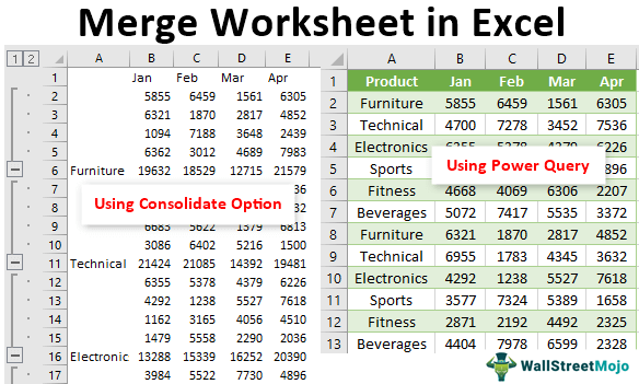
You are free to use this image on your website, templates, etc, Please provide us with an attribution linkArticle Link to be Hyperlinked
For eg:
Source: Excel Worksheet Merge (wallstreetmojo.com)
Getting the data in multiple worksheets is common but combining all the worksheet data at once is the job of the person who receives the data in different sheets.
Merger Worksheet Using Consolidate Option
The easiest and quickest way to merge multiple worksheets data into one is by using the in-built feature of excel “Consolidate.” For example, look at the below data in Excel sheets.
The above image has four worksheets comprising four different regions’ product-wise sales numbers across months.
We need to create one single sheet from the four above to show all the summary results. Then, follow the below steps to consolidate worksheets.
Step 1: We must first create a new worksheet and name it a “Consolidated Sheet.“
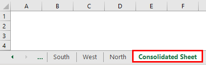
Step 2: We must now place a cursor in the first cell of the worksheet.
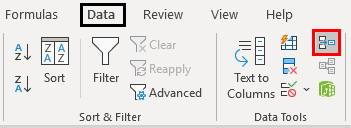
- Then, go to the “Data” tab.
- Click on the “Consolidate” option.
Step 3: As a result, this will open up below the “Consolidate” window.
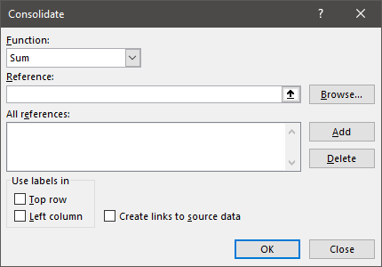
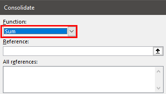
Step 4: Since we are consolidating all the four region data, choose the option of “Sum” under the function drop-down list in excelA drop-down list in excel is a pre-defined list of inputs that allows users to select an option.read more.
Step 5: Next, we need to choose the reference range from the first sheet to the last sheet. Place the cursor inside the reference box, go to the “East” sheet, and choose the data.
Step 6: Click on the “Add” button to add the first reference area.
Now, this is added to the reference list.
Step 7: Next, we have to go to the “South” sheet, and the reference range would have been selected automatically.
Step 8: Click on “Add” again, and the second sheet reference is added to the list. Like this, we can repeat the same for all the sheets.
Now, we have added all four sheets of references. One more thing, while selecting each selected region range, including the row headerExcel Row Header is the grey column on the left side of column 1 in the worksheet that contains the numbers (1, 2, 3, etc.). To hide or reveal row and column headers, press ALT + W + V + H.read more and column header of the data table, to bring the same into the consolidated sheet, we must check the boxes of “Top Row” and “Left Column” and “Create links to Source Data.”
Click on “OK.” We will have a summary table like the one below.
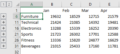
As we can see above, we have two grouped sheets, 1 and 2. If we click on 1, it will show all the region’s consolidated table, and if we click on 2, it will show the breakup of each zone.

It looks fine, but this is not the merging of worksheets. So, merging is combining all the worksheets into one without any calculations; we need to use the “Power Query” option.
Merge Worksheets by Using Power Query
The “Power Query” option is an add-in for ExcelAn add-in is an extension that adds more features and options to the existing Microsoft Excel.read more 2010 and 2013 versions. It is a built-in feature for Excel 2016 onwards versions.
Follow the steps to merge worksheets using Excel’s “Power Query” option.
- We must go to the “Data” tab. Then, from the “Get Data,” select “From File,” “From Workbook.”

- Then, we must select the sheet and then transform it into a Power Query Editor.
We need to convert all the data tables into Excel tables. We have converted each data table into an Excel table and named East, South, West, and North by their region names.
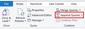
- First, we must go to any of the sheets. Then, under the “Power Query,” click on “Append Queries.”

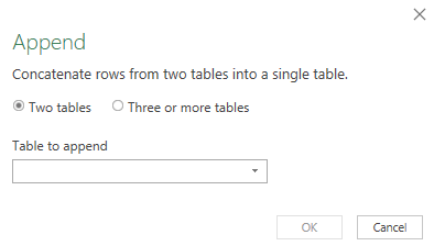
- Now, this will open up the “Append” window.

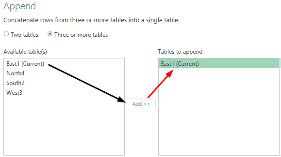
- Here, we need to merge more than one table, so we must choose the “Three or more tables” option.

- Then, select the table “East 1 (Current)” and click on the “Add” button.

For other region tables, we need to repeat the same steps. - After this, click on “OK,” and it will open the “Power Query Editor” window.

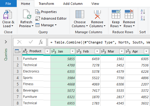
- Finally, we must click on the “Close and Load” option.

Consequently, this will merge all the sheets into one in a new worksheet of the same workbook.

Things to Remember
- The Power Query in excelPower Query is an excel tool used to import data from different sources, transform (change) it as required, and return a refined dataset in the workbook.read more is available for Excel 2010 and 2013 versions as an “Add-in.” From Excel 2016 onwards, this is a built-in tab.
- We can use the “Consolidate” option to consolidate different worksheets into one sheet based on arithmetic calculations.
- We need to convert the data into excel table formatExcel comes with a number of table styles that you may quickly apply to a table format. In Excel, you can design and use a new custom table style of your choice. read more for the “Power Query” merge.
Recommended Articles
This article has been a guide to Excel Worksheet Merge. Here, we discuss merging worksheets into one using the “Consolidate” and “Power Query” options and practical examples. You may learn more about Excel from the following articles: –
- Power Query Tutorial
- Column Merge Excel
- Examples of Combine Cells in Excel
- Merge Tables Excel
- Unmerge Cells Excel