
Summary:
Does merging rows and columns in Excel seems a tough task for you to perform? Read this tutorial to learn different ways to merge rows and columns in Excel.
Microsoft Excel is a very useful application and can be used for performing various tasks. This is the reason Excel provides various useful functions to make the task easy for the users.
One of the most common tasks that everyone needs performing now and then is merging rows and columns.
But the problem is that performing this is not an easy task and Excel does not provide any tool to do this.
This is quite complicated as merging rows and columns in some cases causes data loss.
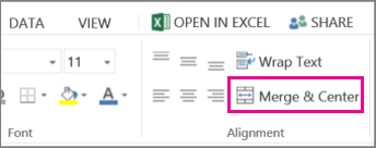
As while trying to combine two or more rows in the worksheet by making use of the Merge & Center button (Home tab > Alignment group), you will start getting the error message:
“The selection contains multiple data values. Merging into one cell will keep the upper-left most data only.”

And if you click OK, merged cells would contain just the value of the top-left cell and as a result, entire other data will be removed.
So this is what leads you to Panic situation!!!
To get rid of this, today in this article I am sharing different ways to easily merge rows and columns in excel without losing any data.
Below check out the fixes on how to merge rows in Excel or how to merge columns in Excel.
To recover Excel data without any data loss, we recommend this tool:
This software will prevent Excel workbook data such as BI data, financial reports & other analytical information from corruption and data loss. With this software you can rebuild corrupt Excel files and restore every single visual representation & dataset to its original, intact state in 3 easy steps:
- Download Excel File Repair Tool rated Excellent by Softpedia, Softonic & CNET.
- Select the corrupt Excel file (XLS, XLSX) & click Repair to initiate the repair process.
- Preview the repaired files and click Save File to save the files at desired location.
There are different methods for combining row and columns text in Excel. Here check the ways one by one to merge data without losing it. First, check how to merge rows in Excel.
Part 1# How To Merge Rows in Excel
When it comes to merging the Excel rows there are two ways that allow you to merge rows data easily.
- Merge Excel rows using a formula
- Combine multiple rows using the Merge Cells add-in
1. How to Merge Multiple Rows using Excel Formulas
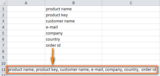
Excel provides various formulas that help you combine data from different rows. Possibly the easiest one is the CONCATENATE function. So here checks out some examples for concatenating numerous rows into one:
- Merge rows with spaces between data: For example =CONCATENATE(B1,” “,B2,” “,B3)
- Combine rows without any space between the values: For example =CONCATENATE(A1,A2,A3)
- Merge rows > separate the values with comma: For Example =CONCATENATE(A1,”, “,A2,”, “,A3)
Now check how the CONCATENATE formula works on the real data.

- On the sheet choose an empty cell and type the formula into it. Type the formula as per the data rows
- And copy the formula across entire other cells in the row.

- Now, simply you are having several data rows merged into one row.
2. How to Combine Rows in Excel using the Merge Cells Add-in

The Merge Cells add-in is used for merging various types of cells in Excel. This allows you to merges the individual cells and also combines data from entire rows or columns.
Please Note: You need to download a merge cell add-ins for third-party sites available online. Search in Google for add-ins.
Follow the given steps to combine two or more rows in your table:
- Choose rows you are looking to merge > click on the Merge Cells icon.
- Now the merge cells dialog window opens with a table or range selected already. And in the upper part of the window, you can see the three basic things:

-
- How you want to join cells – For combining rows of data > choose “column by column“.
- How to separate merged values with – an array of standard separators is available to choose from > comma, space, semicolon, and a line break. So select the separator as per your desire.
- Where you need to place the merged cells > either the top cell or bottom cell.
- Now check the lower part of the Windows to check if you need any additional options:

-
- Clear the content of selected cells – Choose this if need data to remain in the merged cells only.
- Merge all areas in the selection – This option allows you to merge rows in two or more non-adjacent ranges.
- Skip empty cells and Wrap text – Well, these are self-explanatory.
- Lastly, Create a backup copy of the worksheet – This option is checked by default. It is just a precaution that keeps you on the safe side and prevents the risk of data loss.
- Click the Merge button > to check the result – possible the merged rows of data separated by line breaks.
So, these are the two ways that allow you to merge rows in Excel without any data loss. Now, check out the ways on how to combine two columns in Excel.
Part 2# How To Merge Columns In Excel

Here check out the 3 ways to merge data from several columns into one without using VBA macro.
- Merge two columns using formulas
- Combine columns data via NotePad
- The fastest way to join multiple columns
1. Merge Two Columns using Excel Formulas
1. Into your table > insert a new column > in the column header place the mouse pointer > right-click the mouse > select Insert from the context menu. Name the newly added columns for eg. – “Full Name”

2. In the cell D2, write the formula: =CONCATENATE(B2,” “,C2). The B2 and C2 are the addresses of First Name and Last Name. And in the formula, the quotation marks “” is the separator that will be inserted between merged names any other symbol can be used as a separator e.g. a comma.

3. Just like this, join data from several cells into one by making use of any separator of your choice.

4. Simply, copy the formula to other cells of the Full Name column. If the First name or the Last name is deleted, then the corresponding data in the Full name Column will also be gone.

5. Next, try converting the formula to a value so that you can remove the unnecessary columns from the Excel worksheet. Choose entire cells with data in the merged column (choose the first cell in “Full Name” Column > press Ctrl +Shift + Arrow Down)
6. Now copy the contents of the columns to clipboard > right click on the cell in the same column (“Full Name”) > choose “Paste Special” context menu > choose “Values” radio button > click OK.

7. Now remove “First Name” & “Last Name” columns that are not required. Click the column B header > press and hold Ctrl > click column C header.

8. After that make a right-click on any selected columns > select Delete from the context menu.
9. This is it, now you have successfully merged the names from 2 columns into one.

2. Combine columns Data via Notepad
This is another way that allows you to merge several columns. Here you don’t need any formulas. This is suitable for combining adjacent columns to make use of the same delimiter for all of them.
For Example: If looking for combining 2 columns with First Names and Last Names into one:
- Choose both columns you need to merge: Click B1 > press Shift + ArrrowRight for choosing C1 > then hit Ctrl + Shift + ArrowDown for choosing entire data cells with data in two columns.

- And copy data to clipboard > open Notepad > insert data from the clipboard to the Notepad

- Then copy tab character to clipboard > hit Tab right in Notepad > hit Ctrl + Shift + LeftArrow > press Ctrl + X.
- After that Replace Tab characters in Notepad with the separator, you require.
- Hit Ctrl + H for opening the “Replace” dialog box > paste the Tab character from the clipboard in Find what field > type the separator Space, comma etc in “Replace with” field. Hit the Replace All button > to close the dialog box press Cancel

- Now select the entire text in the Notepad and copy it to Clipboard.
- Then switch back to Excel worksheet (press Alt + Tab) > choose B1 cell and paste text from Clipboard to your table.

- And rename column B to “Full Name“ and remove the “Last name” column.
So, this is the second way that allows you to merge columns in Excel without any data loss.
3. Join Columns Using Merge Cells Add-in For Excel
This is the easiest and quickest way for combining data from numerous Excel columns into one. Just make use of the third party merge cells add-in for Excel.
And with the merge cells add-in you can merge data from many cells by using any separator you like (for example carriage return or line break). With this, you can join row by row, column by column, or merge data from the selected cell into one without any loss.
There are many third-party add-ins online sites that allow you to download the add-ins and merge the cells easily in just a few clicks.
Conclusion:
So this is all about merging rows and columns in Excel without any data loss.
Follow the given steps to combine text in rows and columns easily.
Hope the given different steps will allow you to perform the task easily in the rows and column. Here I have described different methods of merging rows and columns data in Excel without any data loss.
So make use of anyone that you find easy for you.
However if in case you come to face any issue or data loss situation in Excel then make use of the MS Excel Repair Tool. This is the best tool that allows you to repair and recover data from the corrupted, damaged Excel file.
Additionally, you can learn advanced Excel to become more productive and easily utilize Excel functions and formulas.

Priyanka is an entrepreneur & content marketing expert. She writes tech blogs and has expertise in MS Office, Excel, and other tech subjects. Her distinctive art of presenting tech information in the easy-to-understand language is very impressive. When not writing, she loves unplanned travels.
Содержание
- Merge and unmerge cells
- Merge cells
- Unmerge cells
- Merge cells
- Unmerge cells
- Split text from one cell into multiple cells
- Merge cells
- Unmerge cells
- Need more help?
- How to Merge Cells, Columns and Rows in Excel
- Merging Cells
- Merging Rows
- Merge Columns
- An Aside About the Concatenate Function
- Wrapping Up
- How to merge and unmerge cells in Microsoft Excel in 4 ways, to clean up your data and formatting
- How to merge cells in Excel
- How to merge and center
- How to merge across
- How to merge cells
- How to unmerge cells
Merge and unmerge cells
You can’t split an individual cell, but you can make it appear as if a cell has been split by merging the cells above it.

Merge cells
Select the cells to merge.
Select Merge & Center.
Important: When you merge multiple cells, the contents of only one cell (the upper-left cell for left-to-right languages, or the upper-right cell for right-to-left languages) appear in the merged cell. The contents of the other cells that you merge are deleted.
Unmerge cells
Select the Merge & Center down arrow.
Select Unmerge Cells.
You cannot split an unmerged cell. If you are looking for information about how to split the contents of an unmerged cell across multiple cells, see Distribute the contents of a cell into adjacent columns.
After merging cells, you can split a merged cell into separate cells again. If you don’t remember where you have merged cells, you can use the Find command to quickly locate merged cells.
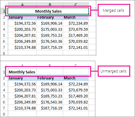
Merging combines two or more cells to create a new, larger cell. This is a great way to create a label that spans several columns.
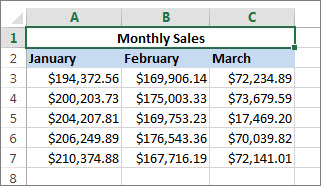
In the example here, cells A1, B1, and C1 were merged to create the label “Monthly Sales” to describe the information in rows 2 through 7.
Merge cells
Merge two or more cells by following these steps:
Select two or more adjacent cells you want to merge.
Important: Ensure that the data you want to retain is in the upper-left cell, and keep in mind that all data in the other merged cells will be deleted. To retain any data from those other cells, simply copy it to another place in the worksheet—before you merge.
On the Home tab, select Merge & Center.
If Merge & Center is disabled, ensure that you’re not editing a cell—and the cells you want to merge aren’t formatted as an Excel table. Cells formatted as a table typically display alternating shaded rows, and perhaps filter arrows on the column headings.
To merge cells without centering, click the arrow next to Merge and Center, and then click Merge Across or Merge Cells.
Unmerge cells
If you need to reverse a cell merge, click onto the merged cell and then choose Unmerge Cells item in the Merge & Center menu (see the figure above).
Split text from one cell into multiple cells
You can take the text in one or more cells, and distribute it to multiple cells. This is the opposite of concatenation, in which you combine text from two or more cells into one cell.
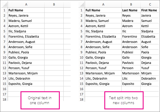
For example, you can split a column containing full names into separate First Name and Last Name columns:
Follow the steps below to split text into multiple columns:
Select the cell or column that contains the text you want to split.
Note: Select as many rows as you want, but no more than one column. Also, ensure that are sufficient empty columns to the right—so that none of your data is deleted. Simply add empty columns, if necessary.
Click Data > Text to Columns, which displays the Convert Text to Columns Wizard.
Click Delimited > Next.
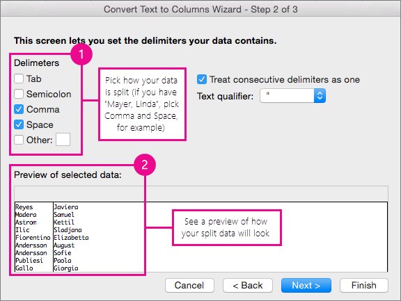
Check the Space box, and clear the rest of the boxes. Or, check both the Comma and Space boxes if that is how your text is split (such as «Reyes, Javiers», with a comma and space between the names). A preview of the data appears in the panel at the bottom of the popup window.
Click Next and then choose the format for your new columns. If you don’t want the default format, choose a format such as Text, then click the second column of data in the Data preview window, and click the same format again. Repeat this for all of the columns in the preview window.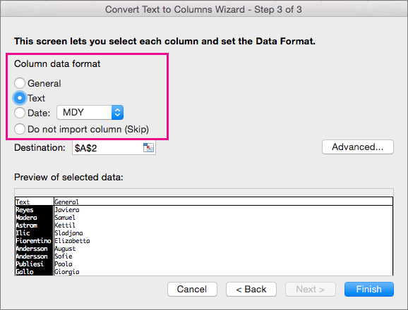
Click the  button to the right of the Destination box to collapse the popup window.
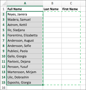
Anywhere in your workbook, select the cells that you want to contain the split data. For example, if you are dividing a full name into a first name column and a last name column, select the appropriate number of cells in two adjacent columns.
Click the  button to expand the popup window again, and then click the Finish button.

Merging combines two or more cells to create a new, larger cell. This is a great way to create a label that spans several columns. For example, here cells A1, B1, and C1 were merged to create the label “Monthly Sales” to describe the information in rows 2 through 7.
Merge cells
Click the first cell and press Shift while you click the last cell in the range you want to merge.
Important: Make sure only one of the cells in the range has data.
Click Home > Merge & Center.
If Merge & Center is dimmed, make sure you’re not editing a cell or the cells you want to merge aren’t inside a table.
Tip: To merge cells without centering the data, click the merged cell and then click the left, center or right alignment options next to Merge & Center.
If you change your mind, you can always undo the merge by clicking the merged cell and clicking Merge & Center .
Unmerge cells
To unmerge cells immediately after merging them, press Ctrl + Z. Otherwise do this:
Click the merged cell and click Home > Merge & Center.
The data in the merged cell moves to the left cell when the cells split.
Need more help?
You can always ask an expert in the Excel Tech Community or get support in the Answers community.
Источник
How to Merge Cells, Columns and Rows in Excel

Depending how you want to format a body of text in Microsoft Excel, you will sometimes have to merge cells. Whatever your reason is, there are a few different techniques you can use. These can help you to achieve the merging of cells, rows, and columns. Some methods will get rid of some of the data in cells, so you have to decide how you want the final result to look beforehand.
Merging Cells
You will find the built-in merge options under the Home tab of Microsoft Excel.

The merge options available are:
- Merge & Center: This option merges cells into one and centers the text. However, only the text from the leftmost cell is kept.
- Merge Across: This option merges cells across from each other into one. All of the rows in a selection chosen to be merged are separated. However, only the text in the leftmost cell of each row is kept.
- Merge Cells: This merges all of the cells in a selection into one. The text is not centered, and only the text from the leftmost cell is kept.
- Unmerge
Consider a case where you made a selection that made up six rows and two columns.

If you choose “Merge & Center,” the result will be centered in the area you selected.

On the other hand, if you choose “Merge Across,” the text in the left cells of the rows that were selected will be kept.

With the “Merge Cells” option, the text in the leftmost cell of the selection is kept and the cells are all fused. The text is not centered in this case.

Merging Rows
If you want to merge rows, then the CONCATENATE function is your best bet. If you wanted to merge a series of rows together into one row where the text is separated by commas, you can use the following formula in a blank cell:

The extra commas and quotation marks are included so that there is a space after the comma that comes after each word in the list.
Merge Columns

The CONCATENATE function is your friend again when it comes to merging columns. In order to merge a group of columns together, you have to pick out the relevant cells in the columns you want to fuse and include them in your CONCATENATE formula. For example, if you had column H and column I with three items in each column, the following formula could be used to merge items together:
An Aside About the Concatenate Function
If you want to have your merged content without spaces, then use the concatenate function like this:

On the other hand, if you want to have your merged content with spaces, you can use the concatenate function like this:

This applies to the merging of both rows and columns.
Wrapping Up
Depending on what you’re doing, you’ll need to format your data differently. This makes merging cells, rows, and columns an invaluable tool. We have covered different techniques here. Feel free to get creative about how you use them. We’ve covered the basics here, but you can do different things like changing up the spacing of your merged content to your preferences. We can also show you how to make your Excel workbook read-only.
William has been fiddling with tech for as long as he remembers. This naturally transitioned into helping friends with their tech problems and then into tech blogging.
Our latest tutorials delivered straight to your inbox
Источник
How to merge and unmerge cells in Microsoft Excel in 4 ways, to clean up your data and formatting
Twitter LinkedIn icon The word «in».
LinkedIn Fliboard icon A stylized letter F.
Flipboard Facebook Icon The letter F.
Email Link icon An image of a chain link. It symobilizes a website link url.
- You can merge cells in Microsoft Excel as a quick and easy way to create titles, or to spread data neatly across columns and rows.
- There are several different types of merges you can perform in Excel, but note that all merges will delete all data except the values in the upper-leftmost cell.
- You can also unmerge cells, but they may then need editing to be realigned and resized correctly.
- Visit Business Insider’s homepage for more stories.
Merging cells is an easy task in Excel, and there are several different default merge styles. You can «Merge and Center» (ideal for a title), «Merge Across» (which merges a cell across columns), or «Merge Cells» (which combines cells across both columns and rows).
In all cases, this will only bring over the content of the cell on the upper-leftmost cell. If there’s other data across the cells you’re trying to merge, you’ll receive a warning saying that merging cells only keeps the upper-left values and discards all others.
How to merge cells in Excel
How to merge and center
1. Highlight the cells you want to merge and center.
2. Click on «Merge & Center,» which should be displayed in the «Alignment» section of the toolbar at the top of your screen.
3. The cells will now be merged with the data centered in the merged cell.
How to merge across
1. Highlight the cells you want to merge.
2. Click on the arrow just next to «Merge and Center.»
3. Scroll down to click on «Merge Across.»
4. The value on the far-left will now be the sole value for the merged cells, though it’ll keep previous alignments steady. For example, a left-aligned value will stay in the left side of the fully merged cell.
How to merge cells
1. Highlight the cells you want to merge.
2. Click on the arrow just next to «Merge and Center.»
3. Scroll down to click on «Merge Cells».
4. This will merge the content of the upper-left cell across all highlighted cells.
How to unmerge cells
1. Highlight the combined cell you want to unmerge.
2. Click on the arrow just next to «Merge and Center.»
3. Click on «Unmerge.»
4. Note that unmerging cells won’t bring back data previously erased by the merging.
Источник
Содержание
- Виды объединения
- Способ 1: объединение через окно форматирования
- Способ 2: использование инструментов на ленте
- Способ 3: объединение строк внутри таблицы
- Способ 4: объединение информации в строках без потери данных
- Способ 5: группировка
- Вопросы и ответы

При работе с таблицами иногда приходится менять их структуру. Одним из вариантов данной процедуры является объединение строк. При этом, объединенные объекты превращаются в одну строчку. Кроме того, существует возможность группировки близлежащих строчных элементов. Давайте выясним, какими способами можно провести подобные виды объединения в программе Microsoft Excel.
Читайте также:
Как объединить столбцы в Excel
Как объединить ячейки в Экселе
Виды объединения
Как уже было сказано выше, существуют два основных вида объединения строк – когда несколько строчек преобразуются в одну и когда происходит их группировка. В первом случае, если строчные элементы были заполнены данными, то они все теряются, кроме тех, которые были расположены в самом верхнем элементе. Во втором случае, физически строки остаются в прежнем виде, просто они объединяются в группы, объекты в которых можно скрывать кликом по значку в виде символа «минус». Есть ещё вариант соединения без потери данных с помощью формулы, о котором мы расскажем отдельно. Именно, исходя из указанных видов преобразований, формируются различные способы объединения строчек. Остановимся на них подробнее.
Способ 1: объединение через окно форматирования
Прежде всего, давайте рассмотрим возможность объединения строчек на листе через окно форматирования. Но прежде, чем приступить к непосредственной процедуре объединения, нужно выделить близлежащие строки, которые планируется объединить.
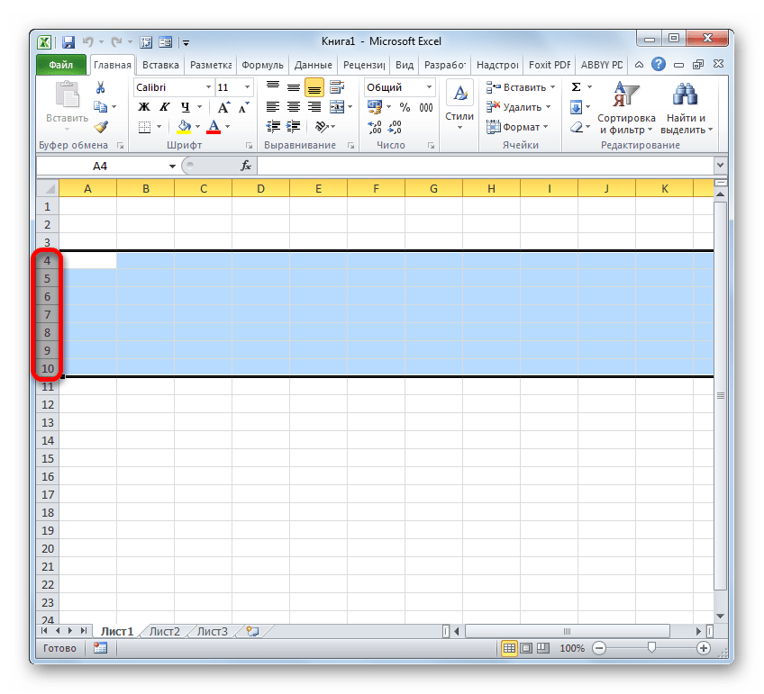
- Для выделения строчек, которые нужно объединить, можно использовать два приёма. Первый из них заключается в том, что вы зажимаете левую кнопку мыши и проводите по секторам тех элементов на вертикальной панели координат, которые нужно объединить. Они будут выделены.

Также, все на той же вертикальной панели координат можно кликнуть левой кнопкой мыши по номеру первой из строк, подлежащей объединению. Затем произвести щелчок по последней строчке, но при этом одновременно зажать клавишу Shift на клавиатуре. Таким образом будет выделен весь диапазон, расположенный между этими двумя секторами.
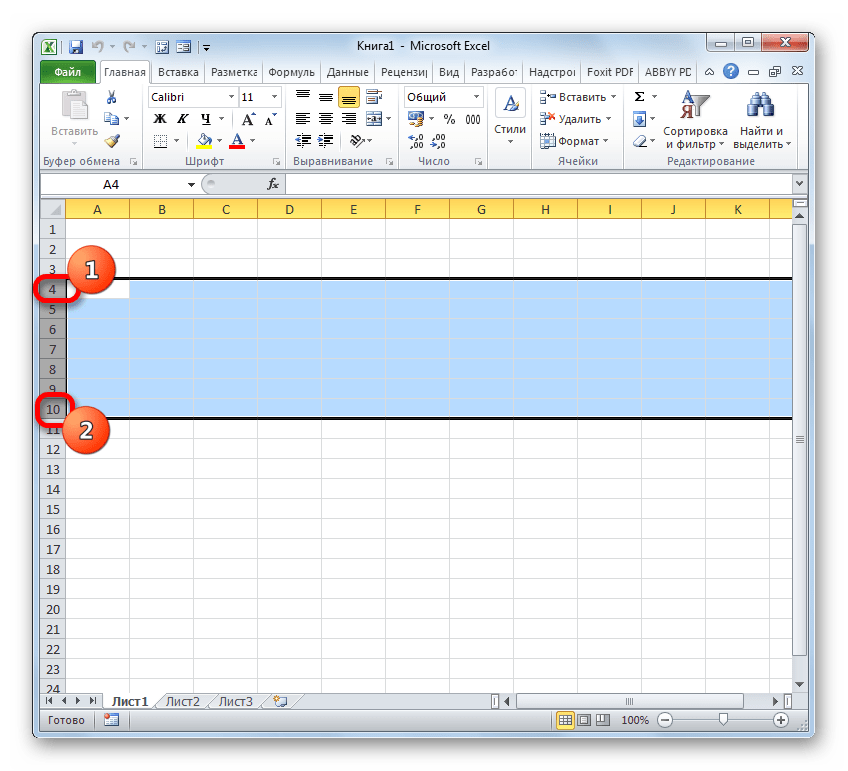
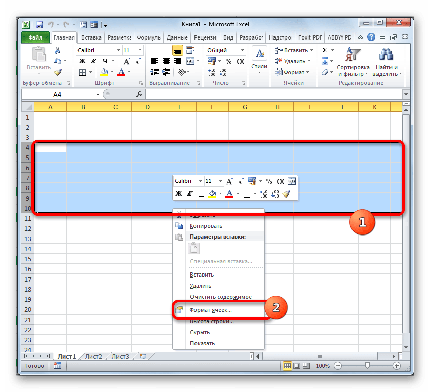
- После того, как необходимый диапазон выделен, можно непосредственно приступать к процедуре объединения. Для этого кликаем правой кнопкой мыши в любом месте выделения. Открывается контекстное меню. Переходим в нем по пункту «Формат ячеек».
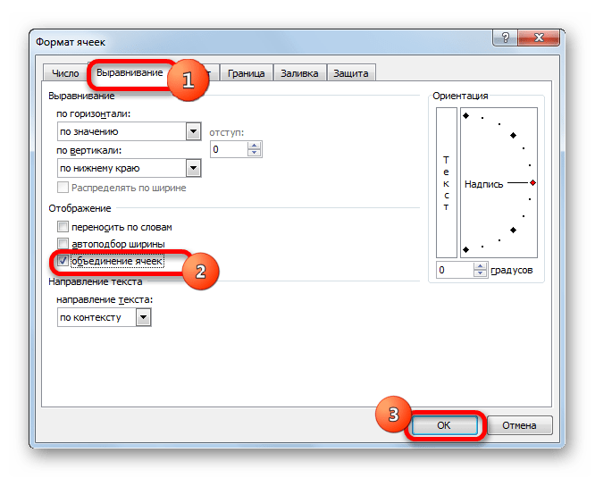
- Выполняется активация окна форматирования. Производим перемещение во вкладку «Выравнивание». Затем в группе настроек «Отображение» следует установить галочку около параметра «Объединение ячеек». После этого можно клацать по кнопке «OK» в нижней части окна.
- Вслед за этим выделенные строчки будут объединены. Причем объединение ячеек произойдет до самого конца листа.

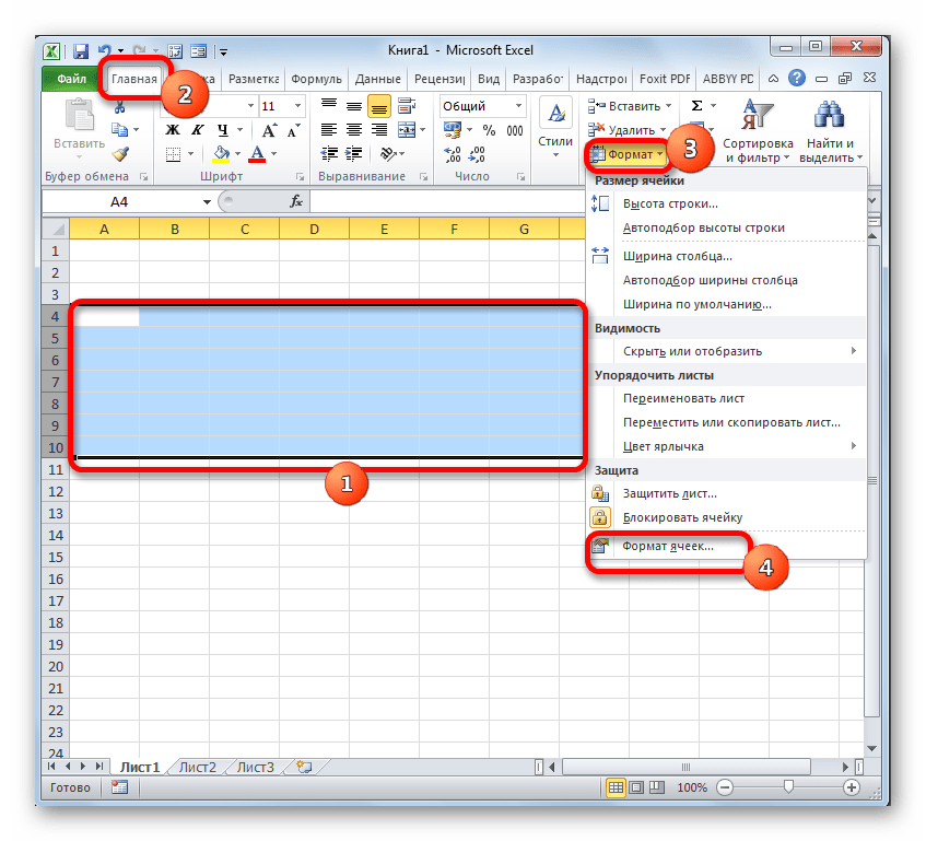
Существуют также альтернативные варианты перехода к окну форматирования. Например, после выделения строк, находясь во вкладке «Главная», можно кликнуть по значку «Формат», расположенному на ленте в блоке инструментов «Ячейки». Из раскрывшегося списка действий следует выбрать пункт «Формат ячеек…».
Также, в той же вкладке «Главная» можно кликнуть по косой стрелочке, которая расположена на ленте в правом нижнем углу блока инструментов «Выравнивание». Причем в этом случае переход будет произведен непосредственно во вкладку «Выравнивание» окна форматирования, то есть, пользователю не придется совершать дополнительный переход между вкладками.

Также перейти в окно форматирования можно, произведя нажим комбинации горячих клавиш Ctrl+1, после выделения необходимых элементов. Но в этом случае переход будет осуществлен в ту вкладку окна «Формат ячеек», которая посещалась в последний раз.

При любом варианте перехода в окно форматирования все дальнейшие действия по объединению строчек нужно проводить согласно тому алгоритму, который был описан выше.
Способ 2: использование инструментов на ленте
Также объединение строк можно выполнить, используя кнопку на ленте.
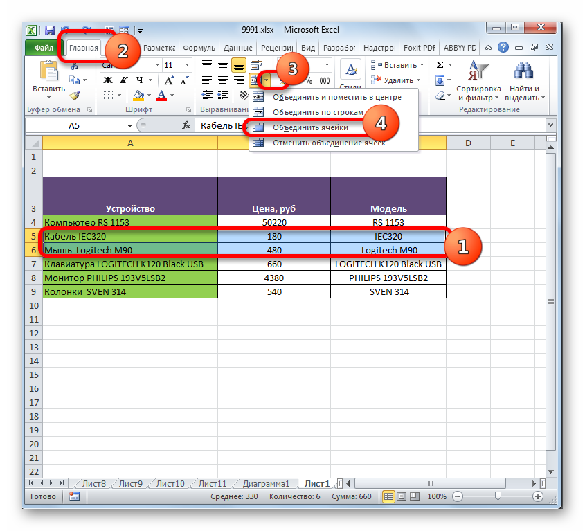
- Прежде всего, производим выделение нужных строчек одним из тех вариантов, о которых шел разговор в Способе 1. Затем перемещаемся во вкладку «Главная» и щелкаем по кнопке на ленте «Объединить и поместить в центре». Она располагается в блоке инструментов «Выравнивание».
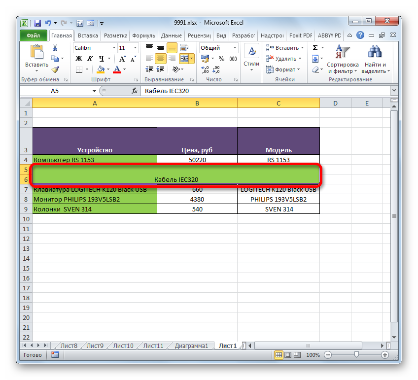
- После этого выделенный диапазон строк будет объединен до конца листа. При этом все записи, которые будут вноситься в эту объединенную строчку, расположатся по центру.


Но далеко не во всех случаях требуется, чтобы текст помещался по центру. Что же делать, если его нужно разместить в стандартном виде?
- Производим выделение строк, которые нужно соединить. Перемещаемся во вкладку «Главная». Щелкаем на ленте по треугольнику, который размещен справа от кнопки «Объединить и поместить в центре». Открывается список различных действий. Выбираем наименование «Объединить ячейки».
- После этого строчки будут объединены в одну, а текст или числовые значения разместятся так, как это присуще для их числового формата по умолчанию.


Способ 3: объединение строк внутри таблицы
Но далеко не всегда требуется объединять строчки до конца листа. Намного чаще соединение производится внутри определенного табличного массива. Давайте рассмотрим, как это сделать.
- Выделяем все ячейки строк таблицы, которые мы хотим объединить. Это также можно сделать двумя способами. Первый из них состоит в том, что вы зажимаете левую кнопку мыши и обводите курсором всю область, которая подлежит выделению.
Второй способ будет особенно удобен при объединении в одну строчку крупного массива данных. Нужно кликнуть сразу по верхней левой ячейке объединяемого диапазона, а затем, зажав кнопку Shift – по нижней правой. Можно сделать и наоборот: щелкнуть по верхней правой и нижней левой ячейке. Эффект будет абсолютно одинаковый.
- После того, как выделение выполнено, переходим с помощью любого из вариантов, описанных в Способе 1, в окно форматирования ячеек. В нем производим все те же действия, о которых был разговор выше. После этого строчки в границах таблицы будут объединены. При этом сохранятся только данные, расположенные в левой верхней ячейке объединенного диапазона.

Объединение в границах таблицы можно также выполнить через инструменты на ленте.
- Производим выделение нужных строк в таблице любым из тех двух вариантов, которые были описаны выше. Затем во вкладке «Главная» кликаем по кнопке «Объединить и поместить в центре».
Или щелкаем по треугольнику, расположенному слева от этой кнопки, с последующим щелчком по пункту «Объединить ячейки» раскрывшегося меню.
- Объединение будет произведено согласно тому типу, который пользователь выбрал.

Способ 4: объединение информации в строках без потери данных
Все перечисленные выше способы объединения подразумевают, что после завершения процедуры будут уничтожены все данные в объединяемых элементах, кроме тех, которые разместились в верхней левой ячейке области. Но иногда требуется без потерь объединить определенные значения, расположенные в разных строчках таблицы. Сделать это можно, воспользовавшись специально предназначенной для таких целей функцией СЦЕПИТЬ.
Функция СЦЕПИТЬ относится к категории текстовых операторов. Её задачей является объединение нескольких текстовых строчек в один элемент. Синтаксис этой функции имеет следующий вид:
=СЦЕПИТЬ(текст1;текст2;…)
Аргументы группы «Текст» могут представлять собой либо отдельный текст, либо ссылки на элементы листа, в которых он расположен. Именно последнее свойство и будет использовано нами для выполнения поставленной задачи. Всего может быть использовано до 255 таких аргументов.
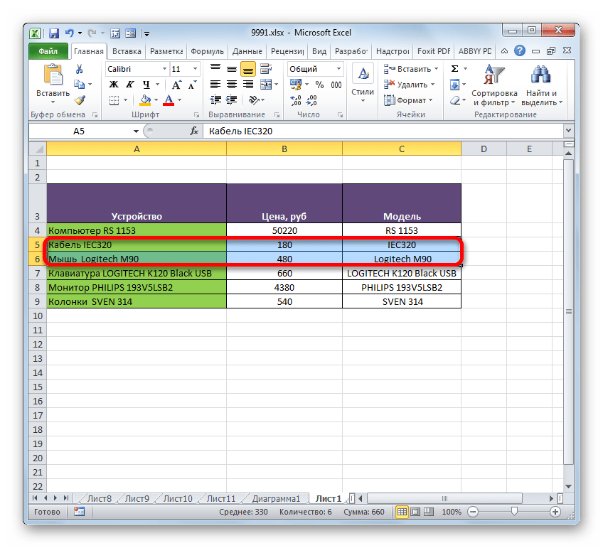
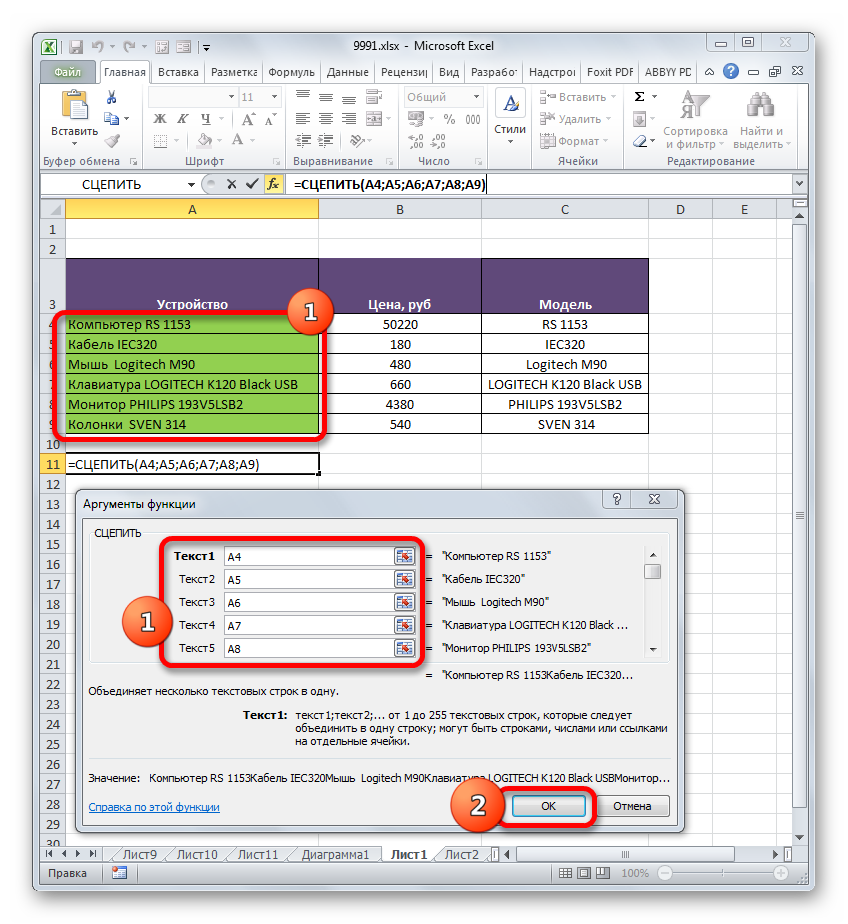
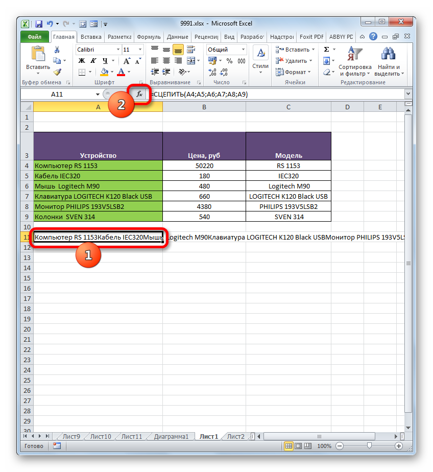
Итак, у нас имеется таблица, в которой указан перечень компьютерной техники с её ценой. Перед нами стоит задача объединить все данные, расположенные в колонке «Устройство», в одну строчку без потерь.
- Устанавливаем курсор в элемент листа, куда будет выводиться результат обработки, и жмем на кнопку «Вставить функцию».
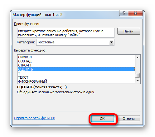
- Происходит запуск Мастера функций. Нам следует переместиться в блок операторов «Текстовые». Далее находим и выделяем название «СЦЕПИТЬ». Затем клацаем по кнопке «OK».
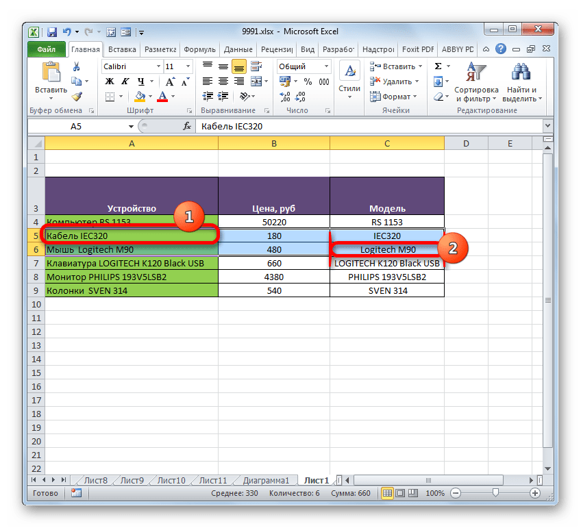
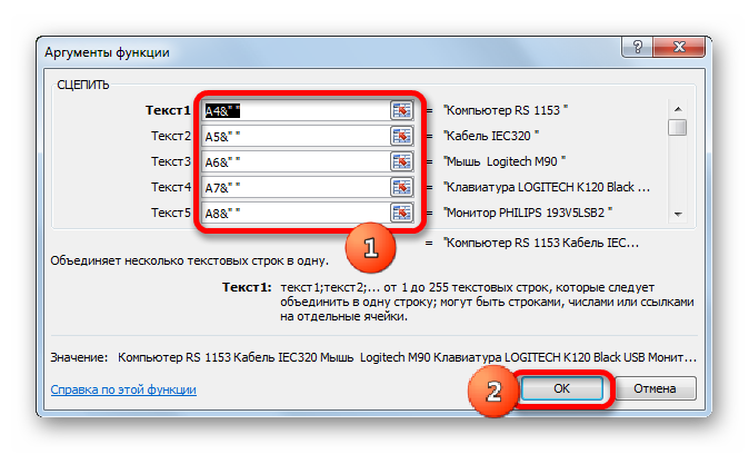
- Появляется окошко аргументов функции СЦЕПИТЬ. По числу аргументов можно использовать до 255 полей с названием «Текст», но для воплощения поставленной задачи нам понадобится столько, сколько строк имеет таблица. В данном случае их 6. Устанавливаем курсор в поле «Текст1» и, произведя зажим левой кнопки мыши, клацаем по первому элементу, содержащему наименование техники в столбце «Устройство». После этого адрес выделенного объекта отобразится в поле окна. Точно таким же образом вносим адреса последующих строчных элементов столбца «Устройство», соответственно в поля «Текст2», «Текст3», «Текст4», «Текст5» и «Текст6». Затем, когда адреса всех объектов отобразились в полях окна, выполняем клик по кнопке «OK».
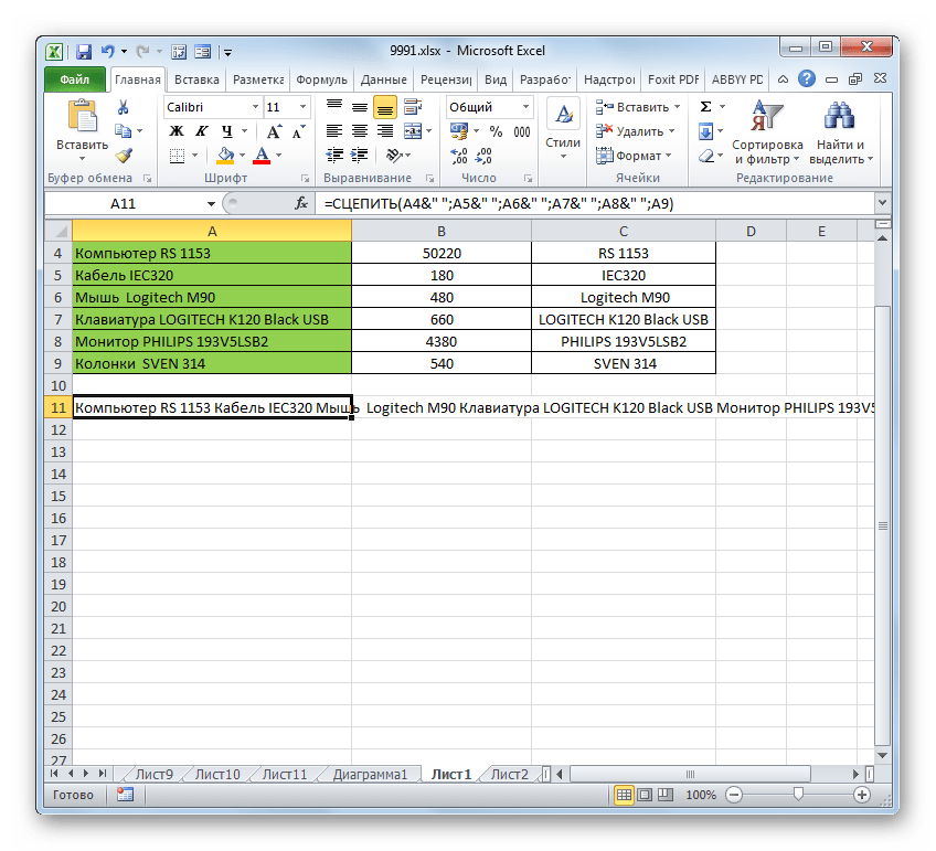
- После этого все данные функция выведет одной строкой. Но, как видим, между наименованиями различных товаров пробел отсутствует, а это нас не устраивает. Для того, чтобы решить данную проблему, выделяем строку, содержащую формулу, и опять жмем на кнопку «Вставить функцию».
- Запускается снова окно аргументов на этот раз без предварительного перехода в Мастер функций. В каждом поле открывшегося окна, кроме последнего, после адреса ячейки дописываем следующее выражение:
&" "Данное выражение – это своеобразный знак пробела для функции СЦЕПИТЬ. Как раз поэтому, в последнее шестое поле его дописывать не обязательно. После того, как указанная процедура выполнена, жмем на кнопку «OK».
- После этого, как видим, все данные не только размещены в одной строке, но и разделены между собой пробелом.

Есть также альтернативный вариант провести указанную процедуру по объединению данных из нескольких строчек в одну без потерь. При этом не нужно даже будет использовать функцию, а можно обойтись обычной формулой.
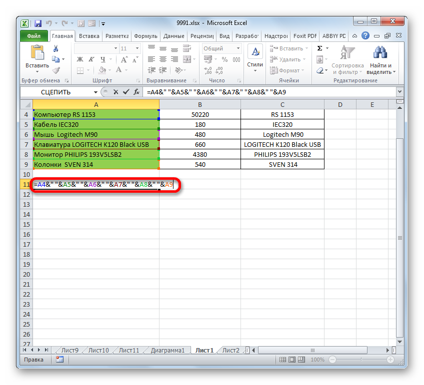
- Устанавливаем знак «=» в строчку, куда будет выводиться результат. Кликаем по первому элементу столбца. После того, как его адрес отобразится в строке формул и в ячейке вывода результата, набираем на клавиатуре следующее выражение:
&" "&После этого кликаем по второму элементу столбца и опять вводим вышеуказанное выражение. Таким образом, обрабатываем все ячейки, данные в которых нужно поместить в одну строку. В нашем случае получилось такое выражение:
=A4&" "&A5&" "&A6&" "&A7&" "&A8&" "&A9 - Для вывода результата на экран жмем на кнопку Enter. Как видим, несмотря на то, что в данном случае была использована другая формула, конечное значение отображается точно так же, как и при использовании функции СЦЕПИТЬ.

Урок: Функция СЦЕПИТЬ в Экселе
Способ 5: группировка
Кроме того, можно сгруппировать строки без потери их структурной целостности. Посмотрим, как это сделать.
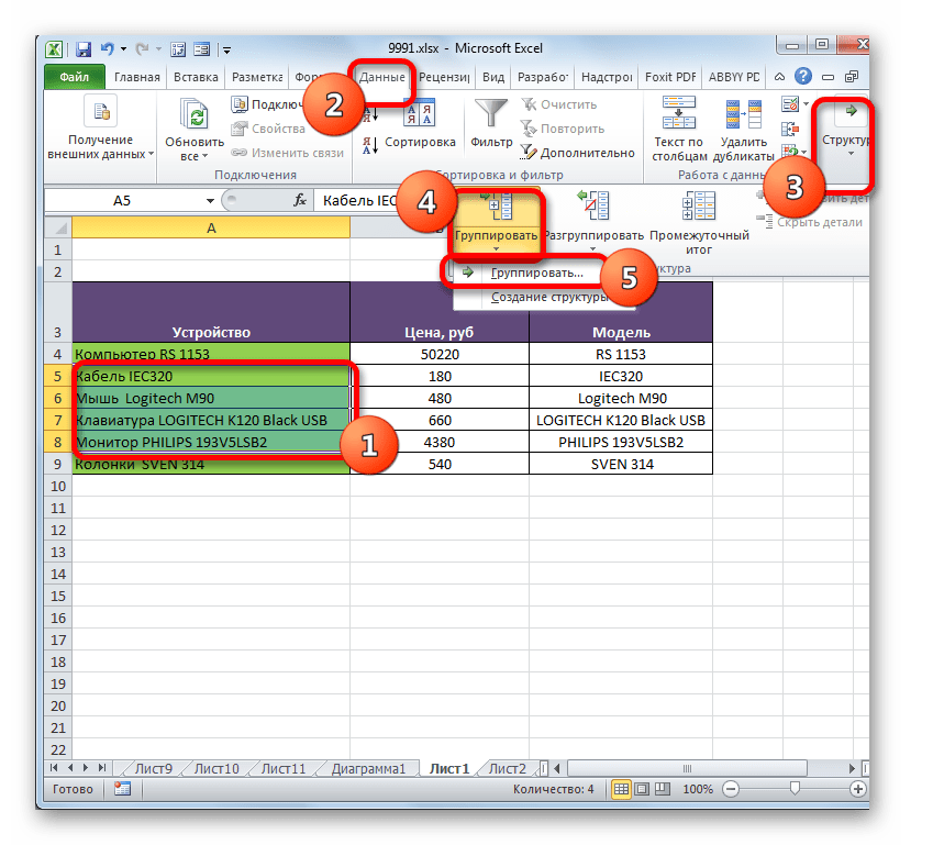
- Прежде всего, выделяем те смежные строчные элементы, которые нужно будет сгруппировать. Можно выделять отдельные ячейки в строках, а не обязательно строчки в целом. После этого перемещаемся во вкладку «Данные». Щелкаем по кнопке «Группировать», которая размещена в блоке инструментов «Структура». В запустившемся небольшом списке из двух пунктов выбираем позицию «Группировать…».
- После этого открывается небольшое окошко, в котором нужно выбрать, что именно мы собираемся группировать: строки или столбцы. Так как нам нужно сгруппировать строчки, то переставляем переключатель в соответствующую позицию и жмем на кнопку «OK».
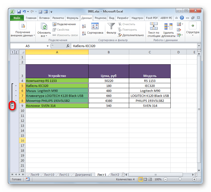
- После выполнения последнего действия выделенные смежные строчки будут соединены в группу. Для того, чтобы её спрятать, достаточно нажать на пиктограмму в виде символа «минус», расположенную слева от вертикальной панели координат.
- Для того, чтобы снова показать сгруппированные элементы, нужно нажать на знак «+» образовавшийся в том же месте, где ранее находился символ «-».


Урок: Как сделать группировку в Экселе
Как видим, способ объедения строк в одну зависит от того, какой именно вид объединения пользователю нужен, и что он хочет получить в итоге. Можно произвести объединение строк до конца листа, в пределах таблицы, выполнить процедуру без потери данных при помощи функции или формулы, а также провести группировку строчек. Кроме того, существуют отдельные варианты выполнения данных задач, но на их выбор уже влияют только предпочтения пользователя с точки зрения удобства.
Merge and unmerge cells
You can’t split an individual cell, but you can make it appear as if a cell has been split by merging the cells above it.
Merge cells
-
Select the cells to merge.
-
Select Merge & Center.
Important: When you merge multiple cells, the contents of only one cell (the upper-left cell for left-to-right languages, or the upper-right cell for right-to-left languages) appear in the merged cell. The contents of the other cells that you merge are deleted.
Unmerge cells
-
Select the Merge & Center down arrow.
-
Select Unmerge Cells.
Important:
-
You cannot split an unmerged cell. If you are looking for information about how to split the contents of an unmerged cell across multiple cells, see Distribute the contents of a cell into adjacent columns.
-
After merging cells, you can split a merged cell into separate cells again. If you don’t remember where you have merged cells, you can use the Find command to quickly locate merged cells.
Merging combines two or more cells to create a new, larger cell. This is a great way to create a label that spans several columns.
In the example here, cells A1, B1, and C1 were merged to create the label “Monthly Sales” to describe the information in rows 2 through 7.
Merge cells
Merge two or more cells by following these steps:
-
Select two or more adjacent cells you want to merge.
Important: Ensure that the data you want to retain is in the upper-left cell, and keep in mind that all data in the other merged cells will be deleted. To retain any data from those other cells, simply copy it to another place in the worksheet—before you merge.
-
On the Home tab, select Merge & Center.

Tips:
-
If Merge & Center is disabled, ensure that you’re not editing a cell—and the cells you want to merge aren’t formatted as an Excel table. Cells formatted as a table typically display alternating shaded rows, and perhaps filter arrows on the column headings.
-
To merge cells without centering, click the arrow next to Merge and Center, and then click Merge Across or Merge Cells.
Unmerge cells
If you need to reverse a cell merge, click onto the merged cell and then choose Unmerge Cells item in the Merge & Center menu (see the figure above).
Split text from one cell into multiple cells
You can take the text in one or more cells, and distribute it to multiple cells. This is the opposite of concatenation, in which you combine text from two or more cells into one cell.
For example, you can split a column containing full names into separate First Name and Last Name columns:
Follow the steps below to split text into multiple columns:
-
Select the cell or column that contains the text you want to split.
-
Note: Select as many rows as you want, but no more than one column. Also, ensure that are sufficient empty columns to the right—so that none of your data is deleted. Simply add empty columns, if necessary.
-
Click Data >Text to Columns, which displays the Convert Text to Columns Wizard.
-
Click Delimited > Next.
-
Check the Space box, and clear the rest of the boxes. Or, check both the Comma and Space boxes if that is how your text is split (such as «Reyes, Javiers», with a comma and space between the names). A preview of the data appears in the panel at the bottom of the popup window.
-
Click Next and then choose the format for your new columns. If you don’t want the default format, choose a format such as Text, then click the second column of data in the Data preview window, and click the same format again. Repeat this for all of the columns in the preview window.
-
Click the
button to the right of the Destination box to collapse the popup window. -
Anywhere in your workbook, select the cells that you want to contain the split data. For example, if you are dividing a full name into a first name column and a last name column, select the appropriate number of cells in two adjacent columns.
-
Click the
button to expand the popup window again, and then click the Finish button.
Merging combines two or more cells to create a new, larger cell. This is a great way to create a label that spans several columns. For example, here cells A1, B1, and C1 were merged to create the label “Monthly Sales” to describe the information in rows 2 through 7.
Merge cells
-
Click the first cell and press Shift while you click the last cell in the range you want to merge.
Important: Make sure only one of the cells in the range has data.
-
Click Home > Merge & Center.
If Merge & Center is dimmed, make sure you’re not editing a cell or the cells you want to merge aren’t inside a table.
Tip: To merge cells without centering the data, click the merged cell and then click the left, center or right alignment options next to Merge & Center.
If you change your mind, you can always undo the merge by clicking the merged cell and clicking Merge & Center.
Unmerge cells
To unmerge cells immediately after merging them, press Ctrl + Z. Otherwise do this:
-
Click the merged cell and click Home > Merge & Center.
The data in the merged cell moves to the left cell when the cells split.
Need more help?
You can always ask an expert in the Excel Tech Community or get support in the Answers community.
See Also
Overview of formulas in Excel
How to avoid broken formulas
Find and correct errors in formulas
Excel keyboard shortcuts and function keys
Excel functions (alphabetical)
Excel functions (by category)
Need more help?
Want more options?
Explore subscription benefits, browse training courses, learn how to secure your device, and more.
Communities help you ask and answer questions, give feedback, and hear from experts with rich knowledge.
Depending how you want to format a body of text in Microsoft Excel, you will sometimes have to merge cells. Whatever your reason is, there are a few different techniques you can use. These can help you to achieve the merging of cells, rows, and columns. Some methods will get rid of some of the data in cells, so you have to decide how you want the final result to look beforehand.
Merging Cells
You will find the built-in merge options under the Home tab of Microsoft Excel.
The merge options available are:
- Merge & Center: This option merges cells into one and centers the text. However, only the text from the leftmost cell is kept.
- Merge Across: This option merges cells across from each other into one. All of the rows in a selection chosen to be merged are separated. However, only the text in the leftmost cell of each row is kept.
- Merge Cells: This merges all of the cells in a selection into one. The text is not centered, and only the text from the leftmost cell is kept.
- Unmerge
Consider a case where you made a selection that made up six rows and two columns.
If you choose “Merge & Center,” the result will be centered in the area you selected.
On the other hand, if you choose “Merge Across,” the text in the left cells of the rows that were selected will be kept.
With the “Merge Cells” option, the text in the leftmost cell of the selection is kept and the cells are all fused. The text is not centered in this case.
Merging Rows
If you want to merge rows, then the CONCATENATE function is your best bet. If you wanted to merge a series of rows together into one row where the text is separated by commas, you can use the following formula in a blank cell:
=CONCATENATE(A2,", ",A2,", ",A3,", ",A4,", ",A5,", ",A6...)
The extra commas and quotation marks are included so that there is a space after the comma that comes after each word in the list.
The CONCATENATE function is your friend again when it comes to merging columns. In order to merge a group of columns together, you have to pick out the relevant cells in the columns you want to fuse and include them in your CONCATENATE formula. For example, if you had column H and column I with three items in each column, the following formula could be used to merge items together:
=CONCATENATE(H1,", ",H2,", ",H3,", ",I1,", ",I2,", ",I3)
An Aside About the Concatenate Function
If you want to have your merged content without spaces, then use the concatenate function like this:
=CONCATENATE(A2,A2,A3,A4,A5,A6)
On the other hand, if you want to have your merged content with spaces, you can use the concatenate function like this:
=CONCATENATE(A2," ",A2," ",A3," ",A4," ",A5," ",A6)
This applies to the merging of both rows and columns.
Wrapping Up
Depending on what you’re doing, you’ll need to format your data differently. This makes merging cells, rows, and columns an invaluable tool. We have covered different techniques here. Feel free to get creative about how you use them. We’ve covered the basics here, but you can do different things like changing up the spacing of your merged content to your preferences. We can also show you how to make your Excel workbook read-only.

William Elcock
William has been fiddling with tech for as long as he remembers. This naturally transitioned into helping friends with their tech problems and then into tech blogging.
Subscribe to our newsletter!
Our latest tutorials delivered straight to your inbox
Sometimes, user wants to merge rows and columns in their Excel sheet. But this is not an easy task, it is quite complicated. Hence, in this blog you will read the method to merge rows and columns in Excel without losing data but if you need help, then contact Microsoft Support team through www.office.com/setup.

click here to download
Method To Merge Rows and Columns in Excel:
1. Merge Rows in Excel:
1. Merge Multiple Rows using Excel Formulas:
Excel gives you so many formulas which help you combine data from different rows. One of the formula is CONCATENATE function. For Concatenate numerous rows into one is to Merge rows with spaces between data, you can combine rows without any space between the values and you can merge rows and then separate the values with comma.
For this, on the sheet you can choose an empty cell and then you should type the formula into it. Here, you should type the formula as per the data rows. And then you should copy the formula across other cells in the row. Now, several data rows merged into one row.
2. Combine Rows in Excel by using the Merge Cells Add-in:
For this, first you should choose rows which you are looking to merge and then click on the Merge Cells icon. Here, you will see the merge cells dialog window opens with a table or range. Then in the upper part of the window, you have to select Merge selected cell- in this you should choose “column by column“. In the separate merged values with – you can choose from comma, space, semicolon, and a line break. Then in the Where you want to place the merged cells, you should select the top cell.
After this, in the lower part of the Windows you should select the from the following options: Clear the content of selected cells, Merge all areas in the selection, Skip empty cells and Wrap text and from the Create a backup copy of the worksheet.
Now, you should click on the Merge button and then check the result – the merged rows are separated by line breaks.
2. Merge Columns In Excel:
1. Merge Two Columns By using Excel Formulas:
First, in your table, you should insert a new column, then in the column header place the mouse pointer and then right-click the mouse. After this, just select Insert from the context menu. You have to name the newly added columns. Now, in the cell D2, you should write the formula: =CONCATENATE(B2,” “,C2). Then in the formula, the quotation marks “” is the separator which will be inserted between merged names. There are other symbol which you can use as a separator. Here, you can join data from several cells into one just by making use of any separator. After this, you should copy the formula to other cells of the Full Name column. At this point, you should convert the formula to a value so that you can easily remove the unnecessary columns from the worksheet. Now, you should copy the contents of the columns to clipboard and then right click on the cell in the same column and after this, you should choose “Paste Special” context menu and then choose “Values” radio button and just click OK button. Here, you should remove “First Name” & “Last Name” columns which are not required. After this, you should right-click on any selected columns and then select Delete from the context menu. Finally, you have merged the names from 2 columns into one. www.office.com/setup
2. Combine Columns Data via Notepad:
First, you should choose both columns which you want to merge: For this, you should click B1 and then press Shift + ArrrowRight for choosing C1 and then press Ctrl + Shift + ArrowDown for selecting entire data cells with data in two columns.
Then, you have to copy data to clipboard and choose open Notepad and after this, insert data from the clipboard to the Notepad. Now, you should copy tab character to clipboard and press Tab right in Notepad and then tap on Ctrl + Shift + LeftArrow and then press Ctrl + X. At this point, you should replace Tab characters in Notepad with the separator. Here, you should press Ctrl + H for opening the “Replace” dialog box and then paste the Tab character from the clipboard in Find what field and then type Space separator in “Replace with” field. Now, you should tap on the Replace All button and then close the dialog box and then press Cancel. At this point, you should select the entire text in the Notepad and then copy it to Clipboard. Here, you should switch back to Excel worksheet (press Alt + Tab) and then choose B1 cell and just paste text from Clipboard to your table. At last, you should rename column B to “Full Name“ and then remove the “Last name” column.
For more help, just contact to the support team of MS Office through office.com/setup.
visit here this link: Quick Way To Resolve MS Office Error Code 0x4004f00c:
Merged cells are one of the most popular options used by beginner spreadsheet users.
But they have a lot of drawbacks that make them a not so great option.
In this post, I’ll show you everything you need to know about merged cells including 8 ways to merge cells.
I’ll also tell you why you shouldn’t use them and a better alternative that will produce the same visual result.
What is a Merged Cell
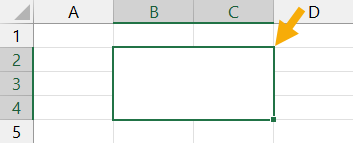
A merged cell in Excel combines two or more cells into one large cell. You can only merge contiguous cells that form a rectangular shape.
The above example shows a single merged cell resulting from merging 6 cells in the range B2:C4.
Why You Might Merge a Cell
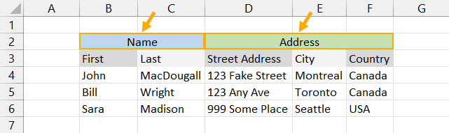
Merging cells is a common technique used when a title or label is needed for a group of cells, rows or columns.
When you merge cells, only the value or formula in the top left cell of the range is preserved and displayed in the resulting merged cell. Any other values or formulas are discarded.
The above example shows two merged cells in B2:C2 and D2:F2 which indicates the category of information in the columns below. For example the First and Last name columns are organized with a Name merged cell.
Why is the Merge Command Disabled?
On occasion, you might find the Merge & Center command in Excel is greyed out and not available to use.
There are two reasons why the Merge & Center command can become unavailable.
- You are trying to merge cells inside an Excel table.
- You are trying to merge cells in a protected sheet.
Cells inside an Excel table can not be merged and there is no solution to enable this.
If most of the other commands in the ribbon are greyed out too, then it’s likely the sheet is protected. In order to access the Merge option, you will need to unprotect the worksheet.
This can be done by going to the Review tab and clicking the Unprotect Sheet command.
If the sheet has been protected with a password, then you will need to enter it in order to unprotect the sheet.
Now you should be able to merge cells inside the sheet.
Merged Cells Only Retain the Top Left Values
Warning before you start merging cells!
If the cells contain data or formulas, then you will lose anything not in the upper left cell.
A warning dialog box will appear telling you Merging cells only keeps the upper-left value and discards other values.
The above example shows the result of merging cells B2:C4 which contains text data. Only the data from cell B2 remains in the resulting merged cells.
If no data is present in the selected cells, then no warning will appear when trying to merge cells.
8 Ways to Merge a Cell
Merging cells is an easy task to perform and there are a variety of places this command can be found.
Merge Cells with the Merge & Center Command in the Home Tab
The easiest way to merge cells is using the command found in the Home tab.
- Select the cells you want to merge together.
- Go to the Home tab.
- Click on the Merge & Center command found in the Alignment section.
Merge Cells with the Alt Hotkey Shortcut
There is an easy way to access the Home tab Merge and Center command using the Alt key.
Press Alt H M C in sequence on your keyboard to use the Merge & Center command.
Merge Cells with the Format Cells Dialog Box
Merging cells is also available from the Format Cells dialog box. This is the menu which contains all formatting options including merging cells.
You can open the Format Cells dialog box a few different ways.
- Go to the Home tab and click on the small launch icon in the lower right corner of the Alignment section.
- Use the Ctrl + 1 keyboard shortcut.
- Right click on the selected cells and choose Format Cells.
Go to the Alignment tab in the Format Cells menu then check the Merge cells option and press the OK button.
Merge Cells with the Quick Access Toolbar
If you use the Merge & Center command a lot, then it might make sense to add it to the Quick Access Toolbar so it’s always readily available to use.
Go to the Home tab and right click on the Merge & Center command then choose Add to Quick Access Toolbar from the options.
This will add the command to your QAT which is always available to use.
A nice bonus that comes with the quick access command is it gets its own hotkey shortcut based on its position in the QAT. When you press the Alt key, Excel will show you what key to press next in order to access the command.
In the above example, the Merge and Center command is the third command in the QAT so the hotkey shortcut is Alt 3.
Merge Cells with Copy and Paste
If you have a merged cell in your sheet already then you can copy and paste it to create more merged cells. This will produce merged cells with the exact same dimensions.
Copy a merged cell using Ctrl + C then paste it into a new location using Ctrl + V. Just make sure the paste area doesn’t overlap an existing merged cell.
Merge Cells with VBA
Sub MergeCells()
    Range("B2:C4").Merge
End Sub
The basic command for merging cells in VBA is quite simple. The above code will merge cells B2:C4.
Merge Cells with Office Scripts
function main(workbook: ExcelScript.Workbook) {
	let selectedSheet = workbook.getActiveWorksheet();
	selectedSheet.getRange("B2:C4").merge(false);
	selectedSheet.getRange("B2:C4").getFormat().setHorizontalAlignment(ExcelScript.HorizontalAlignment.center);
}
The above office script will merge and center the range B2:C4.
Merge Cells inside a PivotTable
We can’t make this change for the selected cells because it will affect a PivotTable. Use the field list to change the report. If you are trying to insert or delete cells, move the PivotTable and try again.
If you try to use the Merge and Center command inside a Pivot Table, you will be greeted with the above error message.
You can’t use the Merge & Center command inside a PivotTable, but there is a way to merge cells in the PivotTable options menu.
In order to avail of this option, you will first need to make sure your Pivot Table is in the tabular display mode.
- Select a cell inside your PivotTable.
- Go to the Design tab.
- Click on Report Layout.
- Choose Show in Tabular Form.
Your pivot table will now be in the tabular form where each field you add to the Rows area will be in its own column with data in a displayed in a single row.
Now you can enable the option to show merge cells inside the pivot table.
- Select a cell inside your PivotTable.
- Go to the PivotTable Analyze tab.
- Click on Options.
This will open up the PivotTable Options menu.
Enable the Merge and center cells with labels setting in the PivotTable Options menu.
- Click on the Layout & Format tab.
- Check the Merge and center cells with labels option.
- Press the OK button.
Now as you expand and collapse fields in your pivot table, fields will merge when they have a common label.
10 Ways to Unmerge a Cell
Unmerging a cell is also quick and easy. Most methods involve the same steps as used to merge the cell, but there are a few extra methods worth knowing.
Unmerge Cells with the Home Tab Command
This is the same process as merging cells from the Home tab command.
- Select the merged cells to unmerge.
- Go to the Home tab.
- Click on the Merge & Center command.
Unmerge Cells with the Format Cells Menu
You can unmerge cells from the Format Cells dialog box as well.
Press Ctrl + 1 to open the Format Cells menu then go to the Alignment tab then uncheck the Merge cells option and press the OK button.
Unmerge Cells with the Alt Hot Key Shortcut
You can use the same Alt hot key combination to unmerge a merged cell. Select the merged cell you want to unmerge then press Alt H M C in sequence to unmerge the cells.
Unmerge Cells with Copy and Paste
You can copy the format from a regular single cell to unmerge merged cells.
Find a single cell and use Ctrl + C to copy it, then select the merged cells and press Ctrl + V to paste the cell.
You can use the Paste Special options to avoid overwriting any data when pasting. Press Ctrl + Alt + V then select the Formats option.
Unmerge Cells with the Quick Access Toolbar
This is a great option if you have already added the Merge & Center command to the quick access toolbar previously.
All you need to do is select the merged cells and click on the command or use the Alt hot key shortcut.
Unmerge Cells with the Clear Formats Command
Merged cells are a type of format, so it’s possible to unmerge cells by clearing the format from the cell.
- Select the merged cell to unmerge.
- Go to the Home tab.
- Click on the right part of the Clear button found in the Editing section.
- Select Clear Formats from the options.
Unmerge Cells with VBA
Sub UnMergeCells()
    Range("B2:C4").UnMerge
End Sub
Above is the basic command for unmerging cells in VBA. This will unmerge cells B2:C4.
Unmerge Cells with Office Scripts
Most methods of merging a cell can be performed again to unmerge cells like a toggle switch to merge or unmerge.
However the code in office scripts doesn’t work like this and instead, you will need to remove formatting to unmerge.
function main(workbook: ExcelScript.Workbook) {
	let selectedSheet = workbook.getActiveWorksheet();
	selectedSheet.getRange("B2:C4").clear(ExcelScript.ClearApplyTo.formats);
}
The above code will clear the format in cells B2:C4 and unmerge any merged cells it contains.
Unmerge Cells with the Accessibility Pane
Merged cells create problems for screen readers which is an accessibility issue. Because of this, they are flagged in the Accessibility window pane.
If you know the location of the merged cells, you can select them and go to the Review tab then click on the lower part of the Check Accessibility button and choose Unmerge Cells.
If you don’t know where all the merged cells are, you can open up the accessibility pane and it will show you where there are and you will be able to unmerge them one by one.
Go to the Review tab and click on the top part of the Check Accessibility command to launch the accessibility window pane.
This will show a Merged Cells section which you can expand to see all merged cells in the workbook. Click on the address and Excel will take you to that location.
Click on the downward chevron icon to the right of the address and the Unmerge option can be selected.
Unmerge Cells inside a PivotTable
To unmerge cells inside a pivot table, you just need to disable the setting in the pivot table options menu.
Now you can enable the option to show merge cells inside the pivot table.
- Select a cell inside your PivotTable.
- Go to the PivotTable Analyze tab.
- Click on Options.
- Click on the Layout & Format tab.
- Uncheck the Merge and center cells with labels option.
- Press the OK button.
Merge Multiple Ranges in One Step
In Excel, you can select multiple non-continuous ranges in a sheet by holding the Ctrl key. A nice consequence of this is you can convert these multiple ranges into merged cells in one step.
Hold the Ctrl key while selecting multiple ranges with the mouse. When you’re finished selecting the ranges you can release the Ctrl key and then go to the Home tab and click on the Merge & Center command.
Each range will become its own merged cell.
Combine Data Before Merging Cells
Before you merge any cells which contain data, it’s advised to combine the data since only the data in the top left cell is preserved when merging cells.
There are a variety of ways to do this, but using the TEXTJOIN function is among the easiest and most flexible as it will allow you to separate each cell’s data using a delimiter if needed.
= TEXTJOIN ( ", ", TRUE, B2:C4 )The above formula will join all the text in range B2:C4 going from left to right and then top to bottom. Text in each cell is separated with a comma and space.
Once you have the formula result, you can copy and paste it as a value so that the data is retained when you merge the cells.
How to Get Data from Merged Cells in Excel
A common misconception is that each cell of in the merged range contains the data entered inside.
In fact, only the top left cell will contain any data.
In the above example, the formula references the top left value in the merged range. The result returned is what is seen in the merged range.
In this example, the formula references a cell that is not the top left most cell in the merged range. The result is 0 because this cell is empty and contains no value.
In order to extract data from a merged range, you will always need to reference the top left most cell of the range. Fortunately, Excel automatically does this for you when you select the merged cell in a formula.
How to Find Merged Cells in a Workbook
If you create a bunch of merged cells, you might need to find them all later. Thankfully it’s not a painful process.
This can be done using the Find & Select command.
Go to the Home tab and click on the Find & Select button found in the Editing section, then choose the Find option. This will open the Find and Replace menu
You can also use the Ctrl + F keyboard shortcut.
You don’t need to enter any text to find, you can use this menu to find cells formatted as merged cells.
- Click on the Format button to open the Find Format menu.
- Go to the Alignment tab.
- Check the Merge cells option.
- Press the OK button in the Find Format menu.
- Press the Find All or Find Next button in the Find and Replace menu.
Unmerge All Merged Cells
Fortunately, unmerging all merged cells in a sheet is very easy.
- Select the entire sheet. You can do this two ways.
- Click on the select all button where the column headings meet the row headings.
- Press Ctrl + A on your keyboard.
- Go to the Home tab.
- Press the Merge & Center command.
This will unmerge all the merged cells and leave all the other cells unaffected.
Why You Shouldn’t Merge Cells
There are a lot of reasons why you shouldn’t merge cells.
- You can’t sort data with merged cells.
- You can’t filter data with merged cells.
- You can’t copy and paste values into merged cells.
- It will create accessibility problems for screen readers by changing the order in which text should be read.
This isn’t an exhaustive list, there are likely many more you will come across should you choose to merge cells.
Alternative to Merging a Cell
Good news!
There is a much better alternative than merging cells.
This alternative has none of the negative features that come with merging cells but will still allow you to achieve the same visual look of a merged cell.
It will allow you to display text centered across a range of cells without merging the cells.
Unfortunately, this technique will only work horizontally with one row of cells. There is no option to do something similar with a vertical range of cells.
Select the horizontal range of cells that you would like to center your text across. The first cell should contain the text which is to be centered while the remaining cells should be empty.
This example shows text in cell B2 and the range B2:C2 is selected as the range to center across.
Go to the Home tab and click on the small launch icon in the lower right corner of the Alignment section. This will open up the Format Cells dialog box with the Alignment tab active.
You can also press Ctrl + 1 to open the Format Cells dialog box and navigate to the Alignment tab.
Select Center Across Selection from the Horizontal dropdown options in the Text alignment section.
The text will now appear as though it occupies all cells but it will only exist in the first cell of the centering selection and each cell is still separate.
Pros
- The text appears centered across the selected range similar to a merged cell.
- No negative effects from merged cells.
- Can be used inside an Excel table.
Cons
- Can not center across a vertical range of cells.
Conclusions
There are lots of ways to merge cells in Excel. You can also easily unmerge cells too if you need to.
There are many things to consider when merging cells in Excel.
As you have seen, there are lots of pitfalls to merged cells that you should consider before implementing them in your workbooks.
Do you have a favorite merge method or warning about the dangers of merged cells that are not listed in the post? Let me know about it in the comments.
About the Author
John is a Microsoft MVP and qualified actuary with over 15 years of experience. He has worked in a variety of industries, including insurance, ad tech, and most recently Power Platform consulting. He is a keen problem solver and has a passion for using technology to make businesses more efficient.
Merge and Unmerge Cells in Excel
by Avantix Learning Team | Updated February 19, 2022
Applies to: Microsoft® Excel® 2013, 2016, 2019, 2021 and 365 (Windows)
In Excel, you can merge cells using the Ribbon or the Format Cells dialog box. You can also access merge commands by right-clicking or using keyboard shortcuts. Typically, when a user wants to merge cells, they are trying to place longer headers in one cell (such as January Actual Sales). You can merge cells horizontally across columns or vertically across rows.
If you want to combine data from cells in a worksheet (such as first name and last name) in another cell, you can use the CONCATENATE function, the CONCAT function, the CONCATENATE operator, the TEXTJOIN function or Flash Fill.
Recommended article: How to Combine Cells in Excel using Concatenate (3 Ways)
Do you want to learn more about Excel? Check out our virtual classroom or in-person Excel courses >
Merge cells options are available in the Alignment group on the Home tab in the Ribbon:

Merge cells removes data
If you merge cells with text, only the text in the upper leftmost cell will be used and text in cells to the right (and below) will be removed. If there is data to the right or below in the cells that you are merging, a dialog box appears warning that Excel will keep the upper left values and remove other data.
Merge cells issues
Merged cells cause problems in lists or data sets as Excel will have difficulty associating data with merged headers or merged cells in the data with the correct headers. If you have longer headers in lists or data sets, it’s best to create shorter headers in single cells above the associated data. You will not be able to sort or filter a range with merged cells.
It’s usually better to use Center Across Selection rather than Merge Cells because Excel will not merge the selected cells into one cell, it will simply center the data. This command is available through the Format Cells dialog box. If you are want to merge a title across the top of a worksheet, this is usually the best choice.
Excel merge cells options
Excel merge options include:
- Merge & Center – this will merge the selected cells into one cell and center the data from the upper leftmost cell across the selected cells (if cells to the right or below the upper leftmost cell in the selection contain data, it will be removed).
- Merge Across – this will merge the selected cells into one cell from the leftmost cell across the selected cells (if cells to the right of the leftmost cell in the selection contain data, it will be removed). It does not automatically center the data. Merge Across only works for selections across columns, not rows.
- Merge Cells – this will merge the selected cells into one cell from the upper leftmost cell across the selected cells (if cells to the right or below the upper leftmost cell in the selection contain data, it will be removed). It does not automatically center the data.
- Unmerge Cells – this will unmerge a cell that has been merged.
- Center Across Selection (in the Format Cells dialog box) – this will center the data in the selected cells but will not merge the cells into one cell.
In the following example, cells A1 to D1 have been merged using Merge & Center:

Merge cells using the Ribbon
To merge cells using the Ribbon in Excel:
- Select the cells you want to merge by dragging over the cells or click in the first cell and Shift-click in the last cell. The cells must be adjacent to each other.
- Click the Home tab in the Ribbon.
- In the Alignment group, click the arrow beside Merge & Center. A drop-down menu appears.
- Select the merge option you want. The data in the top leftmost cell or uppermost cell will be merged across the selected cells. Data in the other cells will be removed.
Options to merge cells and unmerge cells appear in the Ribbon when you click the arrow beside Merge & Center:

Merge cells using keyboard shortcuts
If you want to access commands on the Ribbon in Excel using your keyboard, you can press Alt to display key tips and then press the displayed key(s).
To merge cells using keyboard shortcuts (key tips):
- Select the cells you want to merge by dragging over the cells or click in the first cell and Shift-click in the last cell. The cells must be adjacent to each other.
- Press Alt > H > M (this is a sequential shortcut so press Alt then H then M). A drop-down menu with merge options appears in the Ribbon.
- Press the displayed letter for the command you want. The data in the top leftmost cell or uppermost cell will be merged across the selected cells. Data in the other cells will be removed.
The following are the keyboard or key tips shortcuts for merging and unmerging cells:
- Merge & Center – press Alt > H > M > C.
- Merge Across – press Alt + H + M + A.
- Merge Cells – press Alt > H > M > M.
- Unmerge Cells – press Alt > H > M > U.
Key tips appear in the Ribbon when you press Alt > H > M as follows to display merge options:

Unmerge cells
You can unmerge a cell that has been merged.
To unmerge a cell using the Ribbon:
- Select the merged cell.
- Click the Home tab in the Ribbon.
- In the Alignment group, click the arrow beside Merge & Center. A drop-down menu appears.
- Select Unmerge Cells.
You can also use the key tips shortcut method to unmerge a cell.
Use Center Across Selection as an alternative to merge cells
You can also use the Format Cells dialog box in Excel to access the Center Across Selection option. In this case, you are actually applying formatting and the cells are not merged. You can display the Format Cells dialog box easily by right-clicking or by pressing Ctrl + 1 (at the top of the keyboard).
To apply Center Across Selection using the Format Cells dialog box:
- Select the cells with the data you want to center (in the leftmost cell).
- Press Ctrl + 1 or right-click the selected cells and select Format Cells. A dialog box appears.
- Click the Alignment tab.
- From the Horizontal drop-down menu, choose Center Across Selection.
- Click OK.
Center Across Selection appears in the Format Cells dialog box:

Center across selection is really the best option for merged titles.
Subscribe to get more articles like this one
Did you find this article helpful? If you would like to receive new articles, JOIN our email list.
More resources
How to Remove Duplicates in Excel (3 Easy Ways)
How to Lock Cells in Excel (Protect Formulas and Data)
3 Excel Strikethrough Shortcuts to Cross Out Text or Values in Cells
Use Conditional Formatting in Excel to Highlight Dates Before Today (3 Ways)
How to Replace Blank Cells in Excel with Zeros (0), Dashes (-) or Other Values
Related courses
Microsoft Excel: Intermediate / Advanced
Microsoft Excel: Data Analysis with Functions, Dashboards and What-If Analysis Tools
Microsoft Excel: Introduction to Power Query to Get and Transform Data
Microsoft Excel: New and Essential Features and Functions in Excel 365
Microsoft Excel: Introduction to Visual Basic for Applications (VBA)
VIEW MORE COURSES >
Our instructor-led courses are delivered in virtual classroom format or at our downtown Toronto location at 18 King Street East, Suite 1400, Toronto, Ontario, Canada (some in-person classroom courses may also be delivered at an alternate downtown Toronto location). Contact us at info@avantixlearning.ca if you’d like to arrange custom instructor-led virtual classroom or onsite training on a date that’s convenient for you.
Copyright 2023 Avantix® Learning
Microsoft, the Microsoft logo, Microsoft Office and related Microsoft applications and logos are registered trademarks of Microsoft Corporation in Canada, US and other countries. All other trademarks are the property of the registered owners.
Avantix Learning |18 King Street East, Suite 1400, Toronto, Ontario, Canada M5C 1C4 | Contact us at info@avantixlearning.ca