Merge and unmerge cells
You can’t split an individual cell, but you can make it appear as if a cell has been split by merging the cells above it.
Merge cells
-
Select the cells to merge.
-
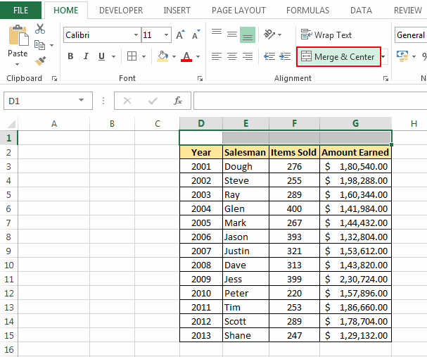
Select Merge & Center.
Important: When you merge multiple cells, the contents of only one cell (the upper-left cell for left-to-right languages, or the upper-right cell for right-to-left languages) appear in the merged cell. The contents of the other cells that you merge are deleted.
Unmerge cells
-
Select the Merge & Center down arrow.
-
Select Unmerge Cells.
Important:
-
You cannot split an unmerged cell. If you are looking for information about how to split the contents of an unmerged cell across multiple cells, see Distribute the contents of a cell into adjacent columns.
-
After merging cells, you can split a merged cell into separate cells again. If you don’t remember where you have merged cells, you can use the Find command to quickly locate merged cells.
Merging combines two or more cells to create a new, larger cell. This is a great way to create a label that spans several columns.
In the example here, cells A1, B1, and C1 were merged to create the label “Monthly Sales” to describe the information in rows 2 through 7.
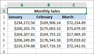
Merge cells
Merge two or more cells by following these steps:
-
Select two or more adjacent cells you want to merge.
Important: Ensure that the data you want to retain is in the upper-left cell, and keep in mind that all data in the other merged cells will be deleted. To retain any data from those other cells, simply copy it to another place in the worksheet—before you merge.
-
On the Home tab, select Merge & Center.
Tips:
-
If Merge & Center is disabled, ensure that you’re not editing a cell—and the cells you want to merge aren’t formatted as an Excel table. Cells formatted as a table typically display alternating shaded rows, and perhaps filter arrows on the column headings.
-
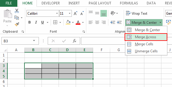
To merge cells without centering, click the arrow next to Merge and Center, and then click Merge Across or Merge Cells.
Unmerge cells
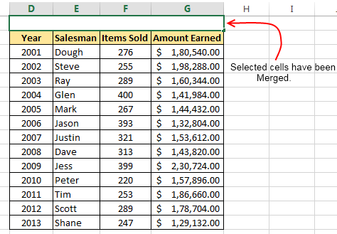
If you need to reverse a cell merge, click onto the merged cell and then choose Unmerge Cells item in the Merge & Center menu (see the figure above).
Split text from one cell into multiple cells
You can take the text in one or more cells, and distribute it to multiple cells. This is the opposite of concatenation, in which you combine text from two or more cells into one cell.
For example, you can split a column containing full names into separate First Name and Last Name columns:
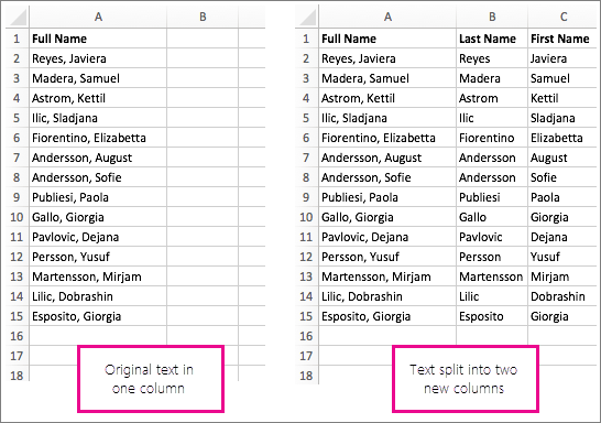
Follow the steps below to split text into multiple columns:
-
Select the cell or column that contains the text you want to split.
-
Note: Select as many rows as you want, but no more than one column. Also, ensure that are sufficient empty columns to the right—so that none of your data is deleted. Simply add empty columns, if necessary.
-
Click Data >Text to Columns, which displays the Convert Text to Columns Wizard.
-
Click Delimited > Next.
-
Check the Space box, and clear the rest of the boxes. Or, check both the Comma and Space boxes if that is how your text is split (such as «Reyes, Javiers», with a comma and space between the names). A preview of the data appears in the panel at the bottom of the popup window.
-
Click Next and then choose the format for your new columns. If you don’t want the default format, choose a format such as Text, then click the second column of data in the Data preview window, and click the same format again. Repeat this for all of the columns in the preview window.
-
Click the
button to the right of the Destination box to collapse the popup window.
-
Anywhere in your workbook, select the cells that you want to contain the split data. For example, if you are dividing a full name into a first name column and a last name column, select the appropriate number of cells in two adjacent columns.
-
Click the
button to expand the popup window again, and then click the Finish button.
Merging combines two or more cells to create a new, larger cell. This is a great way to create a label that spans several columns. For example, here cells A1, B1, and C1 were merged to create the label “Monthly Sales” to describe the information in rows 2 through 7.

Merge cells
-
Click the first cell and press Shift while you click the last cell in the range you want to merge.
Important: Make sure only one of the cells in the range has data.
-
Click Home > Merge & Center.
If Merge & Center is dimmed, make sure you’re not editing a cell or the cells you want to merge aren’t inside a table.
Tip: To merge cells without centering the data, click the merged cell and then click the left, center or right alignment options next to Merge & Center.
If you change your mind, you can always undo the merge by clicking the merged cell and clicking Merge & Center.
Unmerge cells
To unmerge cells immediately after merging them, press Ctrl + Z. Otherwise do this:
-
Click the merged cell and click Home > Merge & Center.
The data in the merged cell moves to the left cell when the cells split.
Need more help?
You can always ask an expert in the Excel Tech Community or get support in the Answers community.
See Also
Overview of formulas in Excel
How to avoid broken formulas
Find and correct errors in formulas
Excel keyboard shortcuts and function keys
Excel functions (alphabetical)
Excel functions (by category)
Need more help?
Want more options?
Explore subscription benefits, browse training courses, learn how to secure your device, and more.
Communities help you ask and answer questions, give feedback, and hear from experts with rich knowledge.
Merged cells are one of the most popular options used by beginner spreadsheet users.
But they have a lot of drawbacks that make them a not so great option.
In this post, I’ll show you everything you need to know about merged cells including 8 ways to merge cells.
I’ll also tell you why you shouldn’t use them and a better alternative that will produce the same visual result.
What is a Merged Cell
A merged cell in Excel combines two or more cells into one large cell. You can only merge contiguous cells that form a rectangular shape.
The above example shows a single merged cell resulting from merging 6 cells in the range B2:C4.
Why You Might Merge a Cell
Merging cells is a common technique used when a title or label is needed for a group of cells, rows or columns.
When you merge cells, only the value or formula in the top left cell of the range is preserved and displayed in the resulting merged cell. Any other values or formulas are discarded.
The above example shows two merged cells in B2:C2 and D2:F2 which indicates the category of information in the columns below. For example the First and Last name columns are organized with a Name merged cell.
Why is the Merge Command Disabled?
On occasion, you might find the Merge & Center command in Excel is greyed out and not available to use.
There are two reasons why the Merge & Center command can become unavailable.
- You are trying to merge cells inside an Excel table.
- You are trying to merge cells in a protected sheet.
Cells inside an Excel table can not be merged and there is no solution to enable this.
If most of the other commands in the ribbon are greyed out too, then it’s likely the sheet is protected. In order to access the Merge option, you will need to unprotect the worksheet.
This can be done by going to the Review tab and clicking the Unprotect Sheet command.
If the sheet has been protected with a password, then you will need to enter it in order to unprotect the sheet.
Now you should be able to merge cells inside the sheet.
Merged Cells Only Retain the Top Left Values
Warning before you start merging cells!
If the cells contain data or formulas, then you will lose anything not in the upper left cell.
A warning dialog box will appear telling you Merging cells only keeps the upper-left value and discards other values.
The above example shows the result of merging cells B2:C4 which contains text data. Only the data from cell B2 remains in the resulting merged cells.
If no data is present in the selected cells, then no warning will appear when trying to merge cells.
8 Ways to Merge a Cell
Merging cells is an easy task to perform and there are a variety of places this command can be found.
Merge Cells with the Merge & Center Command in the Home Tab
The easiest way to merge cells is using the command found in the Home tab.
- Select the cells you want to merge together.
- Go to the Home tab.
- Click on the Merge & Center command found in the Alignment section.
Merge Cells with the Alt Hotkey Shortcut
There is an easy way to access the Home tab Merge and Center command using the Alt key.
Press Alt H M C in sequence on your keyboard to use the Merge & Center command.
Merge Cells with the Format Cells Dialog Box
Merging cells is also available from the Format Cells dialog box. This is the menu which contains all formatting options including merging cells.
You can open the Format Cells dialog box a few different ways.
- Go to the Home tab and click on the small launch icon in the lower right corner of the Alignment section.
- Use the Ctrl + 1 keyboard shortcut.
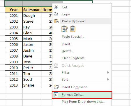
- Right click on the selected cells and choose Format Cells.
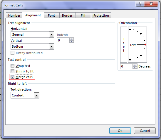
Go to the Alignment tab in the Format Cells menu then check the Merge cells option and press the OK button.
Merge Cells with the Quick Access Toolbar
If you use the Merge & Center command a lot, then it might make sense to add it to the Quick Access Toolbar so it’s always readily available to use.
Go to the Home tab and right click on the Merge & Center command then choose Add to Quick Access Toolbar from the options.
This will add the command to your QAT which is always available to use.
A nice bonus that comes with the quick access command is it gets its own hotkey shortcut based on its position in the QAT. When you press the Alt key, Excel will show you what key to press next in order to access the command.
In the above example, the Merge and Center command is the third command in the QAT so the hotkey shortcut is Alt 3.
Merge Cells with Copy and Paste
If you have a merged cell in your sheet already then you can copy and paste it to create more merged cells. This will produce merged cells with the exact same dimensions.
Copy a merged cell using Ctrl + C then paste it into a new location using Ctrl + V. Just make sure the paste area doesn’t overlap an existing merged cell.
Merge Cells with VBA
Sub MergeCells()
    Range("B2:C4").Merge
End Sub
The basic command for merging cells in VBA is quite simple. The above code will merge cells B2:C4.
Merge Cells with Office Scripts
function main(workbook: ExcelScript.Workbook) {
	let selectedSheet = workbook.getActiveWorksheet();
	selectedSheet.getRange("B2:C4").merge(false);
	selectedSheet.getRange("B2:C4").getFormat().setHorizontalAlignment(ExcelScript.HorizontalAlignment.center);
}
The above office script will merge and center the range B2:C4.
Merge Cells inside a PivotTable
We can’t make this change for the selected cells because it will affect a PivotTable. Use the field list to change the report. If you are trying to insert or delete cells, move the PivotTable and try again.
If you try to use the Merge and Center command inside a Pivot Table, you will be greeted with the above error message.
You can’t use the Merge & Center command inside a PivotTable, but there is a way to merge cells in the PivotTable options menu.
In order to avail of this option, you will first need to make sure your Pivot Table is in the tabular display mode.
- Select a cell inside your PivotTable.
- Go to the Design tab.
- Click on Report Layout.
- Choose Show in Tabular Form.
Your pivot table will now be in the tabular form where each field you add to the Rows area will be in its own column with data in a displayed in a single row.
Now you can enable the option to show merge cells inside the pivot table.
- Select a cell inside your PivotTable.
- Go to the PivotTable Analyze tab.
- Click on Options.
This will open up the PivotTable Options menu.
Enable the Merge and center cells with labels setting in the PivotTable Options menu.
- Click on the Layout & Format tab.
- Check the Merge and center cells with labels option.
- Press the OK button.
Now as you expand and collapse fields in your pivot table, fields will merge when they have a common label.
10 Ways to Unmerge a Cell
Unmerging a cell is also quick and easy. Most methods involve the same steps as used to merge the cell, but there are a few extra methods worth knowing.
Unmerge Cells with the Home Tab Command
This is the same process as merging cells from the Home tab command.
- Select the merged cells to unmerge.
- Go to the Home tab.
- Click on the Merge & Center command.
Unmerge Cells with the Format Cells Menu
You can unmerge cells from the Format Cells dialog box as well.
Press Ctrl + 1 to open the Format Cells menu then go to the Alignment tab then uncheck the Merge cells option and press the OK button.
Unmerge Cells with the Alt Hot Key Shortcut
You can use the same Alt hot key combination to unmerge a merged cell. Select the merged cell you want to unmerge then press Alt H M C in sequence to unmerge the cells.
Unmerge Cells with Copy and Paste
You can copy the format from a regular single cell to unmerge merged cells.
Find a single cell and use Ctrl + C to copy it, then select the merged cells and press Ctrl + V to paste the cell.
You can use the Paste Special options to avoid overwriting any data when pasting. Press Ctrl + Alt + V then select the Formats option.
Unmerge Cells with the Quick Access Toolbar
This is a great option if you have already added the Merge & Center command to the quick access toolbar previously.
All you need to do is select the merged cells and click on the command or use the Alt hot key shortcut.
Unmerge Cells with the Clear Formats Command
Merged cells are a type of format, so it’s possible to unmerge cells by clearing the format from the cell.
- Select the merged cell to unmerge.
- Go to the Home tab.
- Click on the right part of the Clear button found in the Editing section.
- Select Clear Formats from the options.
Unmerge Cells with VBA
Sub UnMergeCells()
    Range("B2:C4").UnMerge
End Sub
Above is the basic command for unmerging cells in VBA. This will unmerge cells B2:C4.
Unmerge Cells with Office Scripts
Most methods of merging a cell can be performed again to unmerge cells like a toggle switch to merge or unmerge.
However the code in office scripts doesn’t work like this and instead, you will need to remove formatting to unmerge.
function main(workbook: ExcelScript.Workbook) {
	let selectedSheet = workbook.getActiveWorksheet();
	selectedSheet.getRange("B2:C4").clear(ExcelScript.ClearApplyTo.formats);
}
The above code will clear the format in cells B2:C4 and unmerge any merged cells it contains.
Unmerge Cells with the Accessibility Pane
Merged cells create problems for screen readers which is an accessibility issue. Because of this, they are flagged in the Accessibility window pane.
If you know the location of the merged cells, you can select them and go to the Review tab then click on the lower part of the Check Accessibility button and choose Unmerge Cells.
If you don’t know where all the merged cells are, you can open up the accessibility pane and it will show you where there are and you will be able to unmerge them one by one.
Go to the Review tab and click on the top part of the Check Accessibility command to launch the accessibility window pane.
This will show a Merged Cells section which you can expand to see all merged cells in the workbook. Click on the address and Excel will take you to that location.
Click on the downward chevron icon to the right of the address and the Unmerge option can be selected.
Unmerge Cells inside a PivotTable
To unmerge cells inside a pivot table, you just need to disable the setting in the pivot table options menu.
Now you can enable the option to show merge cells inside the pivot table.
- Select a cell inside your PivotTable.
- Go to the PivotTable Analyze tab.
- Click on Options.
- Click on the Layout & Format tab.
- Uncheck the Merge and center cells with labels option.
- Press the OK button.
Merge Multiple Ranges in One Step
In Excel, you can select multiple non-continuous ranges in a sheet by holding the Ctrl key. A nice consequence of this is you can convert these multiple ranges into merged cells in one step.
Hold the Ctrl key while selecting multiple ranges with the mouse. When you’re finished selecting the ranges you can release the Ctrl key and then go to the Home tab and click on the Merge & Center command.
Each range will become its own merged cell.
Combine Data Before Merging Cells
Before you merge any cells which contain data, it’s advised to combine the data since only the data in the top left cell is preserved when merging cells.
There are a variety of ways to do this, but using the TEXTJOIN function is among the easiest and most flexible as it will allow you to separate each cell’s data using a delimiter if needed.
= TEXTJOIN ( ", ", TRUE, B2:C4 )The above formula will join all the text in range B2:C4 going from left to right and then top to bottom. Text in each cell is separated with a comma and space.
Once you have the formula result, you can copy and paste it as a value so that the data is retained when you merge the cells.
How to Get Data from Merged Cells in Excel
A common misconception is that each cell of in the merged range contains the data entered inside.
In fact, only the top left cell will contain any data.
In the above example, the formula references the top left value in the merged range. The result returned is what is seen in the merged range.
In this example, the formula references a cell that is not the top left most cell in the merged range. The result is 0 because this cell is empty and contains no value.
In order to extract data from a merged range, you will always need to reference the top left most cell of the range. Fortunately, Excel automatically does this for you when you select the merged cell in a formula.
How to Find Merged Cells in a Workbook
If you create a bunch of merged cells, you might need to find them all later. Thankfully it’s not a painful process.
This can be done using the Find & Select command.
Go to the Home tab and click on the Find & Select button found in the Editing section, then choose the Find option. This will open the Find and Replace menu
You can also use the Ctrl + F keyboard shortcut.
You don’t need to enter any text to find, you can use this menu to find cells formatted as merged cells.
- Click on the Format button to open the Find Format menu.
- Go to the Alignment tab.
- Check the Merge cells option.
- Press the OK button in the Find Format menu.
- Press the Find All or Find Next button in the Find and Replace menu.
Unmerge All Merged Cells
Fortunately, unmerging all merged cells in a sheet is very easy.
- Select the entire sheet. You can do this two ways.
- Click on the select all button where the column headings meet the row headings.
- Press Ctrl + A on your keyboard.
- Go to the Home tab.
- Press the Merge & Center command.
This will unmerge all the merged cells and leave all the other cells unaffected.
Why You Shouldn’t Merge Cells
There are a lot of reasons why you shouldn’t merge cells.
- You can’t sort data with merged cells.
- You can’t filter data with merged cells.
- You can’t copy and paste values into merged cells.
- It will create accessibility problems for screen readers by changing the order in which text should be read.
This isn’t an exhaustive list, there are likely many more you will come across should you choose to merge cells.
Alternative to Merging a Cell
Good news!
There is a much better alternative than merging cells.
This alternative has none of the negative features that come with merging cells but will still allow you to achieve the same visual look of a merged cell.
It will allow you to display text centered across a range of cells without merging the cells.
Unfortunately, this technique will only work horizontally with one row of cells. There is no option to do something similar with a vertical range of cells.
Select the horizontal range of cells that you would like to center your text across. The first cell should contain the text which is to be centered while the remaining cells should be empty.
This example shows text in cell B2 and the range B2:C2 is selected as the range to center across.
Go to the Home tab and click on the small launch icon in the lower right corner of the Alignment section. This will open up the Format Cells dialog box with the Alignment tab active.
You can also press Ctrl + 1 to open the Format Cells dialog box and navigate to the Alignment tab.
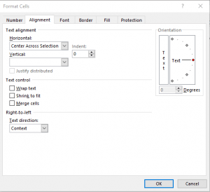
Select Center Across Selection from the Horizontal dropdown options in the Text alignment section.
The text will now appear as though it occupies all cells but it will only exist in the first cell of the centering selection and each cell is still separate.
Pros
- The text appears centered across the selected range similar to a merged cell.
- No negative effects from merged cells.
- Can be used inside an Excel table.
Cons
- Can not center across a vertical range of cells.
Conclusions
There are lots of ways to merge cells in Excel. You can also easily unmerge cells too if you need to.
There are many things to consider when merging cells in Excel.
As you have seen, there are lots of pitfalls to merged cells that you should consider before implementing them in your workbooks.
Do you have a favorite merge method or warning about the dangers of merged cells that are not listed in the post? Let me know about it in the comments.
About the Author
John is a Microsoft MVP and qualified actuary with over 15 years of experience. He has worked in a variety of industries, including insurance, ad tech, and most recently Power Platform consulting. He is a keen problem solver and has a passion for using technology to make businesses more efficient.
Merge and Unmerge Cells in Excel
by Avantix Learning Team | Updated February 19, 2022
Applies to: Microsoft® Excel® 2013, 2016, 2019, 2021 and 365 (Windows)
In Excel, you can merge cells using the Ribbon or the Format Cells dialog box. You can also access merge commands by right-clicking or using keyboard shortcuts. Typically, when a user wants to merge cells, they are trying to place longer headers in one cell (such as January Actual Sales). You can merge cells horizontally across columns or vertically across rows.
If you want to combine data from cells in a worksheet (such as first name and last name) in another cell, you can use the CONCATENATE function, the CONCAT function, the CONCATENATE operator, the TEXTJOIN function or Flash Fill.
Recommended article: How to Combine Cells in Excel using Concatenate (3 Ways)
Do you want to learn more about Excel? Check out our virtual classroom or in-person Excel courses >
Merge cells options are available in the Alignment group on the Home tab in the Ribbon:
Merge cells removes data
If you merge cells with text, only the text in the upper leftmost cell will be used and text in cells to the right (and below) will be removed. If there is data to the right or below in the cells that you are merging, a dialog box appears warning that Excel will keep the upper left values and remove other data.
Merge cells issues
Merged cells cause problems in lists or data sets as Excel will have difficulty associating data with merged headers or merged cells in the data with the correct headers. If you have longer headers in lists or data sets, it’s best to create shorter headers in single cells above the associated data. You will not be able to sort or filter a range with merged cells.
It’s usually better to use Center Across Selection rather than Merge Cells because Excel will not merge the selected cells into one cell, it will simply center the data. This command is available through the Format Cells dialog box. If you are want to merge a title across the top of a worksheet, this is usually the best choice.
Excel merge cells options
Excel merge options include:
- Merge & Center – this will merge the selected cells into one cell and center the data from the upper leftmost cell across the selected cells (if cells to the right or below the upper leftmost cell in the selection contain data, it will be removed).
- Merge Across – this will merge the selected cells into one cell from the leftmost cell across the selected cells (if cells to the right of the leftmost cell in the selection contain data, it will be removed). It does not automatically center the data. Merge Across only works for selections across columns, not rows.
- Merge Cells – this will merge the selected cells into one cell from the upper leftmost cell across the selected cells (if cells to the right or below the upper leftmost cell in the selection contain data, it will be removed). It does not automatically center the data.
- Unmerge Cells – this will unmerge a cell that has been merged.
- Center Across Selection (in the Format Cells dialog box) – this will center the data in the selected cells but will not merge the cells into one cell.
In the following example, cells A1 to D1 have been merged using Merge & Center:
Merge cells using the Ribbon
To merge cells using the Ribbon in Excel:
- Select the cells you want to merge by dragging over the cells or click in the first cell and Shift-click in the last cell. The cells must be adjacent to each other.
- Click the Home tab in the Ribbon.
- In the Alignment group, click the arrow beside Merge & Center. A drop-down menu appears.
- Select the merge option you want. The data in the top leftmost cell or uppermost cell will be merged across the selected cells. Data in the other cells will be removed.
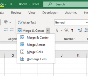
Options to merge cells and unmerge cells appear in the Ribbon when you click the arrow beside Merge & Center:
Merge cells using keyboard shortcuts
If you want to access commands on the Ribbon in Excel using your keyboard, you can press Alt to display key tips and then press the displayed key(s).
To merge cells using keyboard shortcuts (key tips):
- Select the cells you want to merge by dragging over the cells or click in the first cell and Shift-click in the last cell. The cells must be adjacent to each other.
- Press Alt > H > M (this is a sequential shortcut so press Alt then H then M). A drop-down menu with merge options appears in the Ribbon.
- Press the displayed letter for the command you want. The data in the top leftmost cell or uppermost cell will be merged across the selected cells. Data in the other cells will be removed.
The following are the keyboard or key tips shortcuts for merging and unmerging cells:
- Merge & Center – press Alt > H > M > C.
- Merge Across – press Alt + H + M + A.
- Merge Cells – press Alt > H > M > M.
- Unmerge Cells – press Alt > H > M > U.
Key tips appear in the Ribbon when you press Alt > H > M as follows to display merge options:
Unmerge cells
You can unmerge a cell that has been merged.
To unmerge a cell using the Ribbon:
- Select the merged cell.
- Click the Home tab in the Ribbon.
- In the Alignment group, click the arrow beside Merge & Center. A drop-down menu appears.
- Select Unmerge Cells.
You can also use the key tips shortcut method to unmerge a cell.
Use Center Across Selection as an alternative to merge cells
You can also use the Format Cells dialog box in Excel to access the Center Across Selection option. In this case, you are actually applying formatting and the cells are not merged. You can display the Format Cells dialog box easily by right-clicking or by pressing Ctrl + 1 (at the top of the keyboard).
To apply Center Across Selection using the Format Cells dialog box:
- Select the cells with the data you want to center (in the leftmost cell).
- Press Ctrl + 1 or right-click the selected cells and select Format Cells. A dialog box appears.
- Click the Alignment tab.
- From the Horizontal drop-down menu, choose Center Across Selection.
- Click OK.
Center Across Selection appears in the Format Cells dialog box:
Center across selection is really the best option for merged titles.
Subscribe to get more articles like this one
Did you find this article helpful? If you would like to receive new articles, JOIN our email list.
More resources
How to Remove Duplicates in Excel (3 Easy Ways)
How to Lock Cells in Excel (Protect Formulas and Data)
3 Excel Strikethrough Shortcuts to Cross Out Text or Values in Cells
Use Conditional Formatting in Excel to Highlight Dates Before Today (3 Ways)
How to Replace Blank Cells in Excel with Zeros (0), Dashes (-) or Other Values
Related courses
Microsoft Excel: Intermediate / Advanced
Microsoft Excel: Data Analysis with Functions, Dashboards and What-If Analysis Tools
Microsoft Excel: Introduction to Power Query to Get and Transform Data
Microsoft Excel: New and Essential Features and Functions in Excel 365
Microsoft Excel: Introduction to Visual Basic for Applications (VBA)
VIEW MORE COURSES >
Our instructor-led courses are delivered in virtual classroom format or at our downtown Toronto location at 18 King Street East, Suite 1400, Toronto, Ontario, Canada (some in-person classroom courses may also be delivered at an alternate downtown Toronto location). Contact us at info@avantixlearning.ca if you’d like to arrange custom instructor-led virtual classroom or onsite training on a date that’s convenient for you.
Copyright 2023 Avantix® Learning
Microsoft, the Microsoft logo, Microsoft Office and related Microsoft applications and logos are registered trademarks of Microsoft Corporation in Canada, US and other countries. All other trademarks are the property of the registered owners.
Avantix Learning |18 King Street East, Suite 1400, Toronto, Ontario, Canada M5C 1C4 | Contact us at info@avantixlearning.ca
There are various ways you can merge cells in Excel.
One of the most used ways is using the Merge & Center option in the Home tab.
The issue with using Merge & Center is that it can merge the cells, but not the text within these cells (i.e., you lose some data when you merge the cells).
Let’s say we have a data set as shown below:
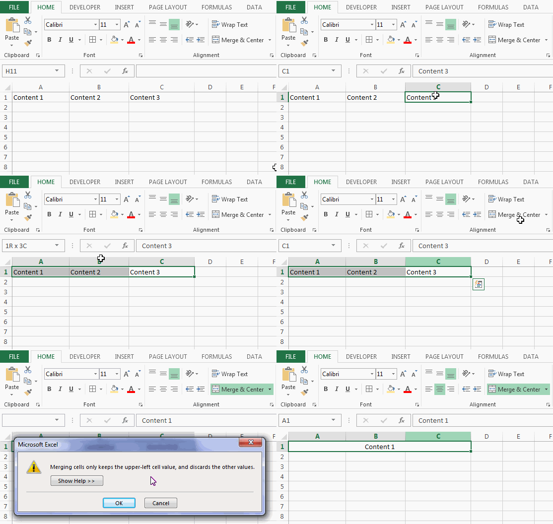
If I select cell A1 and B1 and use the Merge & Center option, it will keep the text from the left-most cell (A1 in this case) and but you will lose the data from all other cells.
Excel is not completely ruthless though – it warns you before this happens.
If you try and merge cells which have text in it, it shows a warning pop-up letting you know of this (as shown below).
If you go ahead and press OK, it will merge the two cells and keep the text from the leftmost cell only. In the above example, it will merge A1 and B1 and will show the text John only.
Merge Cells in Excel Without Losing the Data
If you don’t want to lose the text in from cells getting merged, use the CONCATENATE formula. For example, in the above case, enter the following formula in cell C1: =CONCATENATE(A1,” “,B1)
Here we are combining the cells A1 and B1 and have a space character as the separator. If you don’t want any separator, you can simply leave it out and use the formula =CONCATENATE(A1,B1).
Alternatively, you can use any other separator such as comma or semi-colon.
This result of the CONCATENATE function is in a different cell (in C1). So you may want to copy it (as values) in the cell which you wanted to merge.
You can also use the ampersand sign to combine text. For example, you can also use =A1&” “&B1
The Benefit of Not Merging Cells in Excel
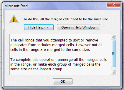
When you use Merge & Center option to merge cells, it robs you of the ability to sort that data set. If you try and sort a data set that has any merged cells, it will show you a pop-up as shown below:
Alternative to Using Merge & Center
If you want to merge cells in different columns in a single row, here is an alternative of Merge & Center – the Center Across Selection option.
Here is how to use it:
- Select the cells that you want to merge.
- Press Control + 1 to open the format cells dialogue box.
- In the Alignment tab, in the Horizontal drop-down, select Center Across Selection.
- Click OK.
This would merge the cells in a way that whatever you enter in the leftmost cell gets centered, however, you can still select each cell individually. This also does not show an error when you try and sort the data.
NOTE: For Center to Across to work, make sure only the leftmost cell has data.
You May Also Like the Following Excel Tutorials:
- How to Unmerge Cells in Excel (3 Easy Ways + Shortcut)
- CONCATENATE Excel Range (with and without separator).
- How to Find Merged Cells in Excel.
- How to Combine Cells in Excel.
- How to Combine Multiple Workbooks into One Excel Workbook.
Knowing the ins and outs of Excel is essential for organizing data, understanding analytics, and getting the most from your marketing efforts. The tool is great for quickly processing vast amounts of data, but it can be overwhelming if you don’t spend the majority of your workday whipping up spreadsheets.
Fortunately, a few basic skills are all you need to put together an easy-to-read spreadsheet. One is knowing how to merge cells in Excel. Whether you’re planning blog articles for the upcoming quarter, creating an email list for a targeted campaign, or designing SEO-friendly Google ads, merging cells is a handy way to organize your information.
To sharpen your skills, we’ll cover several ways to combine cells.
- How to merge two cells
- How to merge and center cells
- How to merge multiple cells
- How to merge cells without losing data
- A shortcut to merge cells
- Why can’t I merge cells?
Don’t want to start from scratch? Use these free Excel templates as a foundation for your own marketing spreadsheets.
Merging is a way to turn two small cells into one new, large cell. This is useful for organizing information and creating headers, without the need to resize individual cells. Here’s how to do it.
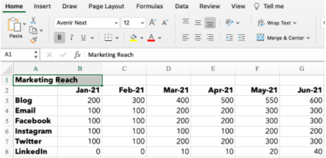
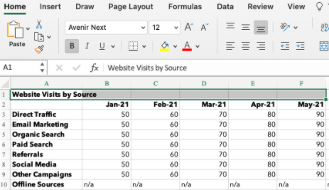
Step 1: Highlight the two adjacent cells you want to merge (I’m merging A1 and B1 in the example).
Source
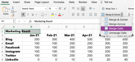
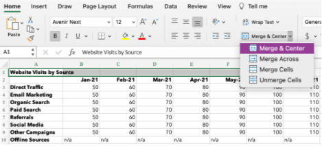
Step 2: Under the Home tab, click the ‘Merge’ icon and choose ‘Merge Cells’.
Source
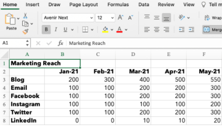
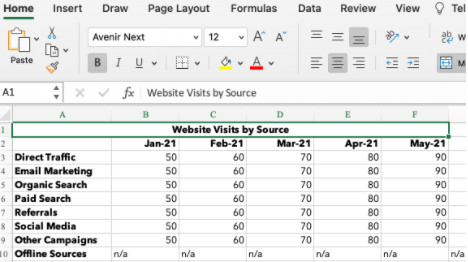
Step 3: That’s it! You’ve merged the cells.
Source
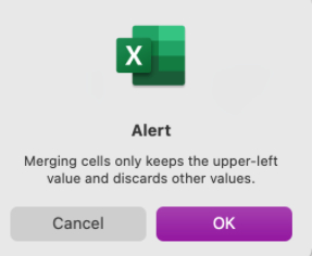
Note: When combining cells, only the data in the upper left cell is saved. Make sure to save the information from the other cell so it’s not lost. If you happen to have data in both A1 and B1, Excel won’t simply wipe it. This alert will pop up:
Source
Don’t want to delete the data? Click ‘Cancel,’ and copy/paste the information into a separate document or cell before merging. If you only need the information in the upper-left cell, click ‘OK’ to merge the cells.
How to Merge and Center Cells in Excel
Say you’re building a marketing report and want your titles to be centered above your data. Merge and center cells by following these steps.
Step 1: Highlight the cells you want to merge.
Source
Step 2: Under the Home tab, click the ‘Merge’ icon and choose ‘Merge & Center.’
Source
Step 3: Your cells will merge and the data will be centered within the cell.
Source
How to Merge Cells in Excel Shortcut
Clicking the correct ‘Merge’ function over and over can be a drag if you need to combine a lot of cells. For fast merging, start by highlighting the cells you want to merge. Then, type the following key combinations.
Excel Shortcuts for Windows
- Merge Cells: ALT H+M+M
- Merge & Center: ALT H+M+C
- Merge Across: ALT H+M+A
- Unmerge Cells: ALT H+M+U
Excel Shortcuts for OS
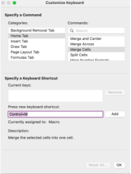
The Apple operating system doesn’t have an ALT key, so you have to set up your own shortcut to merge cells.
- In Excel, click ‘Tools’ under the navigation bar.
- Select ‘Customize Keyboard.’
- A pop-up will appear. Under the header ‘Specify a Command’ there are two columns: Categories and Commands. For Categories, select ‘Home Tab.’ For Commands, select ‘Merge Cells.’
- Select the text box under ‘Press new keyboard shortcut.’ Type the key combination for your shortcut. For example: CONTROL+M.
- Click ‘OK’ to set your shortcut.
- You can now use CONTROL+M to merge cells in Excel.
- Set up additional shortcuts for Merge Across, Merge & Center, or Unmerge.
Source
How to Merge Multiple Cells in Excel
You know the basics, but now you want to get creative and merge more than two cells. Depending on your desired spreadsheet layout, you can use the Merge Across, Merge Cells, or Merge & Center function.
1. Merge Across
This option is used to merge cells within a single row. You can’t use ‘Merge Across’ to combine cells within a column or across multiple rows.
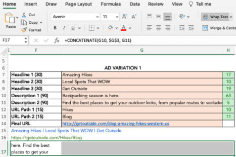
In this example, I’m setting up PPC ads and want to see my description copy in row 17. If I simply resize column F, my table will have too much space between column F and G. Merging multiple cells across row 17 lets me see the copy and keep the table neat.
Step 1: Highlight all the cells you want to merge within the row.
Source
Step 2: Under the Home tab, click the ‘Merge’ icon and choose ‘Merge Across.’
Source
Step 3: The cells merge across the entire highlighted area.
Source
2. Merge & Center
You can merge and center multiple cells across rows and down columns. Just remember the data in the upper-left cell is the only information that will stay once merged. In the example below, I use ‘Merge & Center’ to combine rows 15, 16, and 17 with columns F, G, and H.
Source
Source
3. Merge Cells
The ‘Merge Cells’ function is ideal to combine multiple adjacent cells across rows and columns. It works just like the ‘Merge & Center’ function, except the data will be left-aligned instead of centered after merging.
Source
How to Merge Cells in Excel Without Losing Data
Want to merge cells without losing information from all but the upper left cell? Easy. You can use the ampersand (&) or the CONCATENATE function to combine data from two or more cells.
In the example below, I’m creating copy for Instagram and want to combine the caption with its corresponding link.
Ampersand
Step 1: Choose the cell where you want to put the merged data. Make sure this is separate from the cells you’re merging.
Step 2: Type = in the blank cell and select the first cell to combine.
Step 3: Type & and use » » to leave a space between cell data.
Step 4: Type & again before choosing the next cell. Repeat for all the cells you want to combine. An example formula is =D5&» «&E5.
Step 5: Hit Enter. In the example, you can see how the text from cells D5 and E5 merged into F5.
Source
CONCATENATE or CONCAT
The CONCATENATE function (or CONCAT) is another way to combine two or more text strings together.
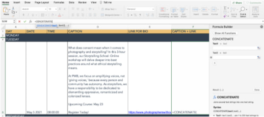
The formula in Excel is =CONCATENATE (text1,text2,…). Text1 is the first cell to merge and can be a text value, number, or cell reference. Text2 is the next item to join. For this function, you can merge up to 255 items or 8,192 characters.
Step 1: Highlight a new blank cell where you want to merge the data.
Step 2: In the formula bar, type =CONCATENATE(
Source
Step 3: A formula builder will pop up, allowing you to choose Text1, Text2, and so on. Select the cells you want to merge, in order from first to last. To include spaces between the cell data, you must include ,» «, within the formula. [i.e. =CONCATENATE(D5,» «,E5)]
Source
Step 4: Hit Enter. The data from your selected cells will be combined in the CONCATENATE cell.
Source
Why Can’t I Merge Cells in Excel?
A lot can go wrong if your formula or formatting isn’t set up correctly. If you’re struggling to merge cells, try these troubleshooting tips.
- Ensure you’re not actively editing a cell you want to merge. The ‘Merge’ icon will be shaded out if you’re in the middle of making changes. To fix this, simply hit ‘Enter’ to stop editing or click onto another cell before clicking back to the cell you’d like to merge.
- Check if one of the cells is part of an Excel table. Tables have a unique format that don’t allow merging. You can tell you’re on a Table if the ‘Chart Design’ or ‘Format’ tabs across the top of your workbook are highlighted in green and the ‘Merge’ icon is shaded out.
- Look at the sharing permissions of the Excel workbook. If it’s not shared with you or is protected, you won’t be able to make any changes or merge cells.
How to Unmerge Cells
Maybe you got a little excited trying out your new skills and merged one cell too many. Don’t panic. Simply unmerge your cells by following these steps.
- Highlight the cells you want to unmerge.
- Under the Home tab, click the ‘Merge’ icon and choose ‘Unmerge Cells.’
- Your cells will go back to the original formatting, but you will have lost the information from before the merge.
- If you need that information, click ‘Command’ + Z (OS) or ‘CTRL’ +Z (Windows) to undo your actions until you see the data pop up.
Merging a cell in excel refers to combining two or more adjacent cells either vertically, horizontally or both ways. Merging excel cells is specifically required when a heading or title has to be centered over an area of a worksheet.
For example, a worksheet contains a balance sheet, a profit and loss account, and a cash flow statement. This data is spread across columns A to H. Hence, to place the title “financial statements” in the center of the data, the cell range A1:H1 has to be merged.
The purpose of merging excel cells is to make the data presentable and readable for the end-user.
Since merging creates a large cell by joining several small ones, the task of resizing individual cells is eliminated. The large cell thus created is displayed across multiple columns or/and rows.
“Merge and center” is an in-built button of merging excel cells placed under the Home tab of Excel. This option merges the cells and not their values. Before merging, it is essential to select the cells to be merged.
Table of contents
- Merge Cells in Excel
- The Techniques of Merge Cells in Excel
- How to Merge Cells in Excel?
- Method #1–“Merge and Center” Drop-down
- Example #1
- Method #2–CONCATENATE Function
- Example #2
- Method #3–Ampersand Operator (&)
- Example #3
- The “Unmerge Cells” Option
- Example #4
- Method #1–“Merge and Center” Drop-down
- An Alternate Method for Center Alignment
- Example #5
- Example #6–Merge Multiple Cells
- Example #7–Merge the Title Cell
- Example #8–Merge two Column Values With the Ampersand Operator
- Example #9–Merge two Column Values With the Concatenate Function
- The Limitations of Merging Excel Cells
- Frequently Asked Questions
- Recommended Articles
You can download this Merge Cells Excel Template here – Merge Cells Excel Template
The Techniques of Merge Cells in Excel
The different ways of merging cells in Excel are listed as follows:
- “Merge and center” drop-down
- CONCATENATE function
- Ampersand operator (&)
How to Merge Cells in Excel?
Let us understand how to merge cells in Excel. We discuss the three merging techniques followed by a few more topics. Each topic consists of an example. Thereafter, some relevant examples are taken up.
Method #1–“Merge and Center” Drop-down
The “merge and centerThe merge and center button is used to merge two or more different cells. When data is inserted into any merged cells, it is in the center position, hence the name merge and center. read more” drop-down consists of various merging options that help combine multiple cells into one. It can be found under the “alignment” group of the Home tab, as shown in the following image.
The different options of the “merge and center” drop-down are explained as follows:
- Merge and center: This merges the selected cells and places the data string in the center. While merging, it retains the text of the upper-leftmost cell only. The text of the remaining merged cells is deleted.
- Merge across: This merges across, implying that the selected cells of the same row are joined together. It merges the values of one row at one time. It retains the text of the upper-leftmost cell only.
- Merge cells: This merges all the selected cells into one single cell. The cells can be selected either horizontally or vertically, or both. It retains the text of the upper-leftmost cell only.
- Unmerge cells: This unmerges the cells implying that the merged cells are split into separate cells again.
Note 1: The difference between the options “merge and center” and “merge cells” is in the alignment of the merged output.
Note 2: The excel shortcutAn Excel shortcut is a technique of performing a manual task in a quicker way.read more for merging (merge and center) is “Alt+H+M+C” and for unmerging is “Alt+H+M+U.” Both the shortcuts must be pressed one by one.
Example #1
The following table shows the first and the last names in columns A and B respectively. We want to merge the two names with the help of the “merge and center” option.
The steps to merge cells with the “merge and center” option are listed as follows:
- Select the cells A2 and B2, which are to be merged.
- From the “merge and center” drop-down in the Home tab, choose “merge and center”.
- A message appears stating that only the upper-leftmost data will be retained. Click “Ok”.
- The cells A2 and B2 are joined with the name “John” in the center. The output is shown in the following image.
The cells A2 and B2 are merged rather than their values. Hence, the text of cell B2 (Abhraham) is deleted while merging cells.
Method #2–CONCATENATE Function
The CONCATENATE functionThe CONCATENATE function in Excel helps the user concatenate or join two or more cell values which may be in the form of characters, strings or numbers.read more combines or concatenates the content of two or more cells. In other words, the values of several cells are joined together in one cell. This function ensures that no data string is lost while merging cell values in excel.
The following image illustrates the CONCATENATE formula for joining the values of cells A2 and B2 with a space in between.
The three parts of the function are explained as follows:
- Part 1 (A2): This is the first cell reference to be joined.
- Part 2 (” “): This is the delimiter “space” that separates the values of the two cells.
- Part 3 (B2): This is the second cell reference to be joined.
Example #2
Working on the data of example #1, we want to merge the first and the last name with a space in between. Use the CONCATENATE function.
The steps to merge cell values with the CONCATENATE formula are listed as follows:
Step 1: Select the cell C2 in which the output is required.
Step 2: Enter the following CONCATENATE formula in cell C2.
“=CONCATENATE(A2,” “,B2)”
Step 3: Press the “Enter” key. The output appears in cell C2, as shown in the following image.
Hence, the values of cells A2 and B2 are merged.
Method #3–Ampersand Operator (&)
The ampersand operator combines different text stringsTo combine text from two or more cells into one cell, select the cell to begin with, then type «=» and select the desired cell to combine, then type «&» and use quotation marks with a space enclosed, and finally select the next required cell to connect and press the enter key.read more by the insertion of “&” within the formula. The formula for combining the values of cells A2 and B2 with a space in between is “=A2&” “&B2”
By using the ampersand, no data string is lost while merging cell values in excel.
Example #3
Working on the data of example #1, we want to join the first and the last name with the help of the ampersand.
The steps to merge cell values with the ampersand operator are listed as follows:
Step 1: Enter the following formula in cell D2.
“=A2&” “&B2”
Step 2: Press the “Enter” key. The output appears in cell D2, as shown in the following image.
Hence, the content of cells A2 and B2 has been merged.
The “Unmerge Cells” Option
Once the cells have been merged, they can be unmerged as well. The “unmerge excel cellsTo unmerge cells in Excel, first select the cells you wish to unmerge, then go to the Home tab and click Unmerge Cells.read more” option (under the “merge and center” drop-down) splits the merged cells, thereby returning the initial layout of cells. However, the data values lost in merging are not restored.
Example #4
Working on the data of example #1, we want to unmerge the merged entries in rows 2 and 4. These entries were merged with the “merge and center” option. Use the “unmerge cells” option for unmerging.
The steps to unmerge data are listed as follows:
Step 1: Select the complete data range A2:B5.
Step 2: Click “unmerge cells” from the “merge and center” drop-down under the Home tab.
Step 3: The cells in rows 2 and 4 have been unmerged. However, the initial data values of column B (shown in example #1) are not restored.
Note: Alternatively, select the merged entries one by one. Thereafter, apply the “unmerge cells” option separately for each entry.
An Alternate Method for Center Alignment
It is difficult to sort (“sort and filter” group of Data tab) merged cells. This is because sorting a merged range in an ascending or a descending order returns a message stating that the cells need to be “identically sized.”
To overcome this limitation, there is an alternate option which does not merge cells but applies the same formatting as the “merge and center” option. In other words, the cells are aligned centrally without any data strings being lost.
The alternate option “center across selection” is available in the “alignment” tab of the “format cells” dialog box.
Example #5
Working on the data of example #1, we want to apply the same formatting as the “merge and center” option without losing any data. Use the “center across selection” alternative.
The steps to format data with the “center across selection” option are listed as follows:
Step 1: Select cells A2 and B2, which are to be formatted.
Step 2: Press “Ctrl+1” together. The “format cellsFormatting cells is an important technique to master because it makes any data presentable, crisp, and in the user’s preferred format. The formatting of the cell depends upon the nature of the data present.read more” dialog box opens, as shown in the following image.
Step 3: Click the “alignment” tab.
Step 4: Select “center across selection” from the drop-down of “horizontal.” Click “Ok.”
Step 5: The formatted output is shown in row 2 of the following image. Hence, the content of cells A2 and B2 is centrally aligned without any loss of data.
Example #6–Merge Multiple Cells
The following table shows the monthly sales (in $) for the years 2016 to 2019. Every year written in column A is followed by two blank cells.
We want to merge the year with the two cells following it so that one cell is created for one year.
The steps to merge multiple cells in Excel are listed as follows:
Step 1: Select the cells A2, A3, and A4.
Step 2: Select “merge and center” from the “merge and center” drop-down of the Home tab. In case the message appears, click “Ok” to merge the cells.
Once merged, apply “middle align” from the “alignment” section of the Home tab. Moreover, bold the text “2016.”
Step 3: Keep the cell containing “2016” selected. Double-click on “format painterFormat painter in Excel is a tool used to copy the same format of a single cell or a group of cells to the other cells. You will find it on the home tab in the clipboard section.read more” under the Home tab.
Step 4: For applying the formatting of “2016” to the remaining cells, press the down arrow key. Excel keeps merging the three excel cells for every year till the “escape” key is pressed.
Example #7–Merge the Title Cell
The following table shows the number of units of a particular product sold by the different sales representatives of an organization. In addition, the date of sale (column A) and the respective region (column C) are also displayed.
The cell B2 shows the title of the table, which is not completely visible currently. We want to merge the cells A2:E2 so that the title is spread across columns A to E.
Step 1: Select the cells A2, B2, C2, D2, and E2 to be merged. The selection can be carried out in any of the following ways:
- Select with the mouse.
- Select by pressing and holding “Shift” along with the relevant arrow keys.
The same is shown in the following image.
Step 2: Select “merge and center” from the alignment group of the Home tab, as shown in the following image.
Step 3: In this case, Excel will not display the message stating that only the upper-leftmost data will be retained. This is because only cell B2 contains data while the remaining cells (A2, C2, D2, and E2) are empty.
However, if the following message does appear, click “Ok.”
Step 4: The cell range A2:E2 is merged. The title “mobile_sales_data_in_different_region” appears in the center of columns A to E.
To make the title stand out, give it a color.
Example #8–Merge two Column Values With the Ampersand Operator
The following table shows the first and last names in columns A and B respectively. We want to perform the following tasks:
a) Merge the data strings of columns A and B with a space in between.
b) Merge the data strings of columns A and B without any spaces.
a) Step 1: Select the cell C2 in which the formula for merging data strings is to be entered.
Step 2: In cell C2, enter the operator “equal to” (=) followed by selecting cell A2 (the first cell to be combined).
Step 3: Enter the ampersand operator (&) followed by a space enclosed within double quotation marks. Enter another (second) ampersand.
Step 4: Select cell B2, which is the second cell to be combined. After entering the complete formula (=A2&” “&B2), press the “Enter” key.
Step 5: The merged output appears in cell C2. Hence, the first and the last names have been combined with a space in between.
Step 6: Drag the formula to the remaining cells. Hence, the full names (with a space in between) for the entire range (C2:C5) are obtained.
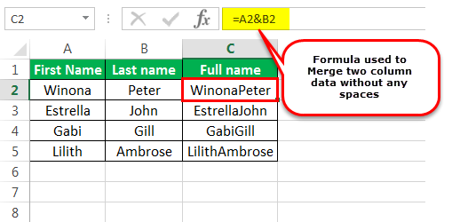
b) We apply the following formula in cell C2.
“=A2&B2”
Press the “Enter” key. Drag the formula to obtain the output in the remaining cells.
The formula merges the values of columns A and B without any spaces between the data strings. The merged output is shown in the following image.
Example #9–Merge two Column Values With the Concatenate Function
Working on the data of example #8, we want to merge the first and the last name with a space between them. Use the CONCATENATE function of Excel.
Step 1: Enter the following formula in cell I2.
“=CONCATENATE(G2,” “,H2)”
Step 2: Press the “Enter” key. The merged output is shown in the following image.
Hence, the names of cells G2 and H2 are joined with a space in between.
Step 3: Drag the formula to obtain the output in the remaining cells. Hence, the full names (with a space in between) for the entire range (I2:I5) are obtained.
The Limitations of Merging Excel Cells
The drawbacks of merging cells in Excel are stated as follows:
- While merging with the “merge and center” drop-down, only the upper-leftmost data is retained and the remaining data is deleted.
- The merging options of the “merge and center” drop-down merge only the excel cells, not their values.
- Once merged, it becomes difficult to sort data whether in an ascending or a descending order.
Note: It is recommended to use the merging options of the “merge and center” drop-down in worksheets that are just meant for presentation purposes. In addition, limit the usage of these options to headings and cell titles only.
Frequently Asked Questions
1. What does it mean to merge cells and how is it done in Excel?
Merging helps combine the data strings of two or more cells. In the process, a single large cell is created from multiple smaller cells. The goal of merging is to improve the presentation of the worksheet.
For example, while storing the contact numbers of employees in Excel, their first and last names (appearing in different columns) have to be merged in one column.
The steps of merging excel cells are listed as follows:
• Select the cells to be merged.
• From the “merge and center” drop-down, choose any one of the three merging options depending on the requirement.
• Click “Ok” in the message that appears.
The selected cells are merged. The value of only the upper-leftmost cell is retained in the merged output.
Note: Before merging with the “merge and center” drop-down, ensure that the entries of all cells are saved in a separate worksheet. This helps retain a copy of the data that is deleted while merging.
2. How to merge cells while retaining data in Excel?
The CONCATENATE function and the ampersand operator (&) help merge cells without losing data. The formulas for the same are mentioned as follows:
To merge cells A1 and B1 with spaces in between:
“=CONCATENATE(A1,” “,B1)” or “=A1&” “&B1”
To merge cells A1 and B1 without spaces in between:
“=CONCATENATE(A1,B1)” or “=A1&B1”
Note 1: While entering the preceding formulas in Excel, ensure that the beginning and the ending double quotation marks are removed.
Note 2: The CONCATENATE function can combine up to 255 strings while there are no such limitations with the usage of the ampersand.
3. How to merge cells in Excel with a comma and hyphen in between?
The CONCATENATE function and the ampersand operator (&) help merge cells with a comma and hyphen in between. The formulas are mentioned as follows:
To merge cells A1 and B1 without spaces but with a comma in between:
“=CONCATENATE(A1,””,B1)” or “=A1&”,”&B1″
To merge cells A1 and B1 with a comma and space in between:
“=CONCATENATE(A1,””,B1)” or “=A1&”, “&B1”
To merge cells A1 and B1 with a hyphen in between:
“=CONCATENATE(A1,”-“,B1)” or “=A1&”-“&B1”
Note: While entering the preceding formulas in Excel, ensure that the beginning and the ending double quotation marks are removed.
Recommended Articles
This has been a guide to merging cells in Excel. Here we discuss how to merge cells in Excel using CONCATENATE and “&” along with Excel examples and a downloadable Excel template. You may also look at these useful Excel articles-
- Merge Worksheet in ExcelMerging data from multiple worksheets into one worksheet is possible with Excel’s «Consolidate» feature. Also, starting with Excel 2010, we can use «Power Query» as a worksheet merger.read more
- Merge Tables in ExcelWe can use a number of different methods to merge tables in Excel, including the VLOOKUP function, the INDEX function, and the MATCH function.read more
- Shortcut to Merge Cells in ExcelIn Excel, there are four shortcuts for merging cells. The most popular method is Alt + H + M + C. Before using the merge command, you must first select the cells.read more
Merging cells in a spreadsheet means taking two or more cells and constructing a single cell out of them. Merging is generally used as a cosmetic trick to center a title over a particular section in a spreadsheet.
The below image clearly shows how a merged cell looks like.
In this post, we will see different ways to merge cells in Excel. But before that let’s understand what makes merging different from concatenation.
How Merging is different from Concatenation?
Many times people confuse between these two words. As I have foretold, Merging is the process of taking two or more cells and constructing a single cell out of them. On the other hand, Concatenation is the process of joining or combining the values from two or more cells.
Recommended Reading: Concatenate Cells in Excel
There are different methods to merge cells in Excel. In the below section we will understand how to do this:
Method 1: Merging multiple cells using the Merge and Centre button in Ribbon
In this method, we will see how to merge cells in excel using the Merge and Centre Button in Excel. Follow the below steps to do this:
- First of all, select the cells that you wish to merge.
- After this navigate to the “Home” tab in the top ribbon and click the “Merge & Centre” button as shown in the below image.
- This will merge all the selected cells and the output will look like the below image.
Method 2: Merging multiple cells using the Format Cells option
In this method, we are going to utilize the Format Cells option to merge the selected cells.
- First of all similar to the previous method, select the cells that you have to merge.
- Next, click the “More Options” button near the “Alignment Settings” on the “Home” Tab as shown.
Alternatively, you can also right-click the selected range and click the “Format Settings” option from the right-click menu.
Tip: You can also use the shortcut Alt + H F A for performing this.
- After this “Format Cells” window will open. Now, in the “Format Cells” window navigate to the “Alignment” tab and check the “Merge” checkbox and click “Ok”.
- This will merge the selected cells.
Method 3: How to Merge cells in Excel using VBA Macro:
If you wish to merge cells using a VBA program then you should try the below codes:
A. VBA Code to merge Selected sells:
Sub Merge_Cells()
If Selection.Cells.Count > 1 Then
 Selection.Merge
 MsgBox "Selected cells Merged!"
Else
 MsgBox "For Merging please select At-Least 2 or More cells!", vbExclamation
End If
End Sub
This code merges the cells that are selected by the user. The code will only execute if the selected cells are greater than 1.
Recommended Reading: IF Statement, Message Box in VBA
A. VBA Code to merge Specified cells:
Sub Merge_Specified_Cells()
Dim Cells As String
On Error GoTo ErrorHandler
Cells = InputBox("Enter the range of cells that you wish to merge." & vbNewLine & _
 "For Example: To Enter a Range A1 to A3 type A1:A3 ")
If ActiveSheet.Range(Cells).Count > 1 Then
 ActiveSheet.Range(Cells).Merge
 MsgBox "Specified cells Merged!"
Else
 MsgBox "For Merging please enter a range containing At-Least 2 or More cells!", vbExclamation
End If
Exit Sub
ErrorHandler:
MsgBox "Entered Range is Invalid!", vbCritical
End Sub
This code asks the user to enter a range, then it merges all the cells present in the specified range.
Recommended Reading: InputBox in VBA, Error Handling in VBA
Merge Cells Across
In the above methods, we have seen how easy it is to merge cells in Excel. But have you thought about how you can merge several individual rows in a range?
The below image will make our objective very clear.
If you select all the cells to be merged and then merge them using any of the methods, the output will be like this:
Option-1: One obvious solution to this would be selecting each row and then merging them individually. This solution will work but if you have a large number of columns then it can be quite cumbersome to merge every row individually.
Option-2: Using the “Merge Across” option. This is an easy way to accomplish our goal and that too in a split second.
Follow the below steps to know how to use this option:
- First of all, select the range that you wish to merge as several individual rows.
- Next, navigate to the “Home” Tab in Ribbon and click the dropdown arrow on the “Merge and centre” button. Now from the menu Click the option “Merge Across” as shown.
- This will merge the cells as several individual rows.
How to Merge without losing data
Do you know that merging can sometimes also result in data loss? Yes, you read that right.
See the below image to know how it happens.
So, what’s the Solution?
The solution to this can be a simple macro that can first concatenate the values in all the selected cells into the upper-leftmost cell and then merge them together.
This boils down to:
Sub JoinAndMerge()
'joins all the content in selected cells
'and puts the resulting text in top most cell
'then merges all cells
Dim outputText As String
Const delim = " "
On Error Resume Next
For Each cell In Selection
 outputText = outputText & cell.Value & delim
Next cell
With Selection
 .Clear
 .Cells(1).Value = outputText
 .Merge
 .HorizontalAlignment = xlGeneral
 .VerticalAlignment = xlCenter
 .WrapText = True
End With
End Sub
This code has been written by Chandoo, you read more ways to tackle this issue on his blog here.
Why Merging sometimes leads to issues:
Merging in excel can cause problems while sorting. If you try to sort your data containing some merged cells, Excel will throw an error saying that, “To do this, all merged cells should be of same size”.
So, I will suggest you minimize the use of Excel’s merging capability.
Recommended Reading: Find merged Cells in Excel
So, this was all from my side. Do let me know in case you come across any issues while trying to merge cells in Excel.
How to Use the Merge & Center button
A great way to customize the layout of your Excel worksheet is to use the Merge & Center feature in Excel.
It is a great way to create a label that spans several columns. This feature will retain the value in the upper-left cell but keep in mind that all data in the other merged cells will be deleted.
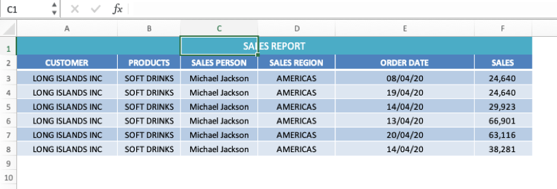
In the example below, you can see that the text “SALES REPORT” is located in a single cell in A1. Let us fix that!
Step 1: Select the cells A1:F1 that you want to merge.
Step 2: Go to Home > ‘Alignment’ group > Merge & Center button
Step 3: The currently selected cells will be merged, and their contents will be center aligned.
Notice that the reference for the 6 merged cells cell points at A1.
By following this step-by-step guide on How to Merge Cells in Excel you can create headers/titles for you report that will make it much easier to understand.
Other Merge & Center Options
When you click on the drop-down arrow beside the Merge & Center button in the Alignment group, you will see it contains a drop-down list with additional options and each one produces a different result:
- Merge Across − When a multi-row range is selected, this command creates multiple merge cells in Excel — one for each row.
- Merge Cells − Merges the selected cells without applying the Center attribute.
- Unmerge Cells −This unmerges the merged cells in Excel and we explain in detail below.
Once you have learned how to merge cells in Excel, you should also know how to unmerge them. In order to Unmerge Cells in Excel
Step 1: Select the cells that you want to unmerge.
Step 2: Click the Merge & Center button or select the Unmerge Cells option from the drop-down menu.
Your data is now unmerged.
NB: Even though this is a fairly simple process to know how to merge cells in Excel, it is not highly recommended, and further below we explain the alternatives to merge cells in Excel.
If any data was lost when the original cells were merged, they will not be restored (unless your select CTRL + Z to undo the last action).
Here are a couple of shortfalls once cells have been merged:
- Excel Functions won’t work on merged cells
- Excel ‘Sort’ command will not work on ranges that contain the Excel merge cells.
- Single column can’t be selected if it contains any merged cells
- Excel Filters cannot be applied
- Dates cannot easily be copy-pasted elsewhere
Here is a video from Microsoft showing merging and unmerging cells in action.
Using Center Across Selection
To achieve the same result as Merge & Center without having the above restrictions, use the Center Across Selection feature. This would merge the cells across columns and still let you select each cell individually. Below we explain how to apply the Center Across Selection:
Step 1: Select the cells A1:F1 that you want to merge.
Step 2: Press Ctrl + 1 to bring up the Format Cells dialog box.
Step 3: Under the Alignment Tab, in the Horizontal drop-down box, select “Center Across Selection”
Step 4: Click OK.
The selected cells are now merged. You can see that even though the data is merged across cell A1: F1, you can still select and refer to each cell individually!
Using the CONCATENATE Function
If you use the above options to merge cells in Excel, it will keep the text at the leftmost cell (A1 in this case) and remove the text from all other cells. If you don’t want to lose the text from the merged cells in Excel, use the CONCATENATE Function (pre Excel 2019), the CONCAT Function (Excel 2019 & Office 365) or the ampersand “&” operator. The CONCATENATE function combines cells in Excel quickly.
There may be times when you are dumped with data in Excel and it is not formatted quite the way you want. Say, you have the First Name and Last Name in different columns and you want to merge them in a single column containing First & Last Name.
Now, if you use Merge & Center or Merge Across Selection, it will delete the text in the second column and only display the First Name as a merged cell. But this is not what you were looking for. Right?
Let me introduce you to the Concatenate Function and the ampersand “&” operator that will merge cells in Excel! This feature should definitely be bookmarked as it will come in handy when cleaning, transforming and analyzing data in Excel.
The Concatenate Function will merge multiple cells into a single cell and keep both values. You can merge or join more than two cells together whether it contains text, numbers, or both.
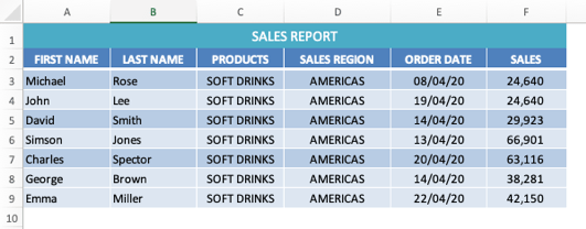
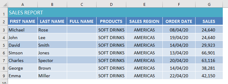
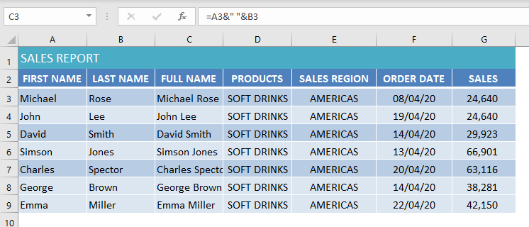
In the SALES REPORT below, you have the First Name in Column A and Last Name in Column B. For reporting and further analysis, you need them to be combined into one column, so it’s best to use the Concatenate function or the “&” Operator for this. It is perfect for when you want to merge cells or combine ‘FIRST NAMES’ with ‘LAST NAMES’ that are in separate columns and merging them into one cell.
Before I get into how to merge cells in Excel, let’s talk about exactly what happens when you try to use Merge & Center here. If you select cells A3 and B3 and then press the “Merge & Center” button, you will see that you end up with an Excel merged cell with only the upper-left cell’s value i.e. the First Name.
To merge cells in Excel without losing any data, you should use the Concatenate Function in Excel. Follow the steps to know how to combine cells in Excel:
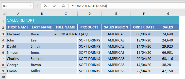
Step 1: Select Column C and press Ctrl + to add a new column. Name this column as “Full Name”.
Step 2: Select Cell C3 and type the formula: =CONCATENATE(A3, B3). Press Enter
Step 3: Copy cell C3 and paste it in remaining cells or drag the fill handle to copy the formula to the other cells below.
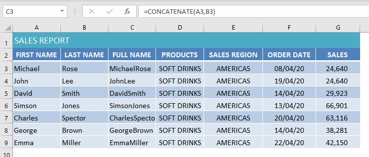
This will merge cells in Excel without losing the data! Below we show you how to make this merged cell look prettier by adding a space between the First & Last Names as well as a line break.
Adding a Space & Line Breaks while Merging Cells
In the FULL NAME column above, you can see that there is no space or any character between the FIRST NAME and the LAST NAME. This mashed-together value of the FULL NAME isn’t a typographical mistake. It is important to understand how to combine cells in Excel including spaces.
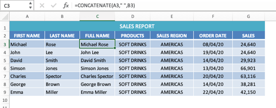
To concatenate this information and include spaces, in the 2nd CONCATENATE function argument, you need to type in double quotation marks and put a space between these quotations i.e. ” “
The edited formula will be =CONCATENATE(A3,” “, B3).
You can replace the space with a dot, comma, or any other character. Simply, replace the space in this function with a character and make sure to enclose the character or text in double quotation marks. With the Concatenate function you also have the option to amend the combination later, whereas you don’t have any such option if you use Merge & Center.
You can also use the ampersand sign, &, to combine cells in Excel. The & operator works just like the CONCATENATE function where you can combine text, numbers, individual cells, etc. Both CONCATENATE and & produce the same results.
Let’s see how to merge cells in Excel using the & operator.
The following examples show the same SALES REPORT but this time I will use & operator to merge cells in Excel.
The formula to be used is = A3&” “&B3
You can see that the result is the same and you can use either the ampersand sign & or the CONCATENATE function, it just depends on what you are more comfortable with.
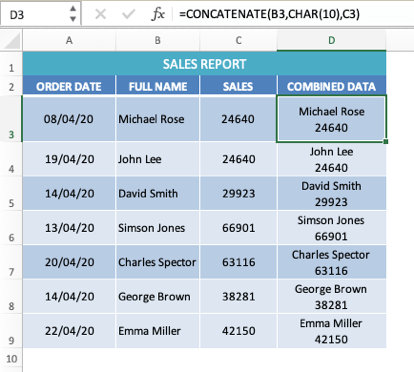
You can also add line breaks while merging cells by using the CHAR(10) function in Excel.
In the following example, the CHAR(10) function is used to add a line break between FULL NAME & SALES. You can use the formula: =CONCATENATE(B3, CHAR(10), C3).
Also, make sure you select the “Wrap Text” option under the Home Tab, otherwise the result will be displayed in the same line only.
You can see that the FULL NAME is displayed on the first line and the second line contains SALES, which is another cool way you can create Excel merged cells.
Bonus Approach – Flash Fill
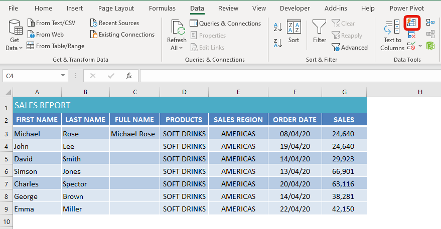
Lastly, there is a BONUS approach to merge cells in Excel with – Flash Fill. It is probably the simplest way to combine cells in Excel and is available in Excel 2013 or later.
Flash Fill is a special tool that analyses the pattern from the existing cells and then automatically extracts the data to the pattern that you set. We can combine the FIRST NAME and LAST NAME from the previous example using Flash Fill.
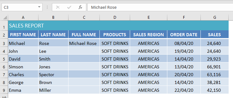
Step 1: You should establish a pattern by typing the FULL NAME in cell C2.
Step 2: Highlight the remaining cell and press the keyboard shortcut Ctrl + E or go to the ribbon menu and select: Data > Flash Fill
Step 3: Excel will sense the pattern you provided in C2, and will fill in the empty cells below, merging the FIRST NAME with the LAST NAME.
If the Flash Fill does not seem to be working for your data, make sure it is turned on.
To turn Flash Fill on, go to Tools > Options > Advanced > Editing Options > check the “Automatically Flash Fill” box.
Excel’s Flash Fill feature is a versatile tool that can be used to merge, split, or clean data. You need to type the first entry for Excel to sense the patterns and then Excel fills in the rest of the data based on the pattern you provided.
In Conclusion
So, the Merge & Center or Center Across Selection features in Excel makes data more visually presentable and highly organized. But it only keeps the contents of the top-left cell and deletes the rest.
This loss of data is a big disadvantage when you merge cells in Excel. To preserve your data in Excel, use the & operator, the CONCATENATE function, or Flash Fill to merges cells’ contents into one cell.
Make sure to download our FREE PDF on the 333 Excel keyboard Shortcuts here:
You can learn more on how to use Excel by viewing our FREE Excel webinar training on Formulas, Pivot Tables and Macros & VBA!
You can follow our YouTube channel to learn more about How To Merge Cells in Excel!
👉 Click Here To Join Our Excel Academy Online Course & Access 1,000+ Excel Tutorials On Formulas, Macros, VBA, Pivot Tables, Dashboards, Power BI, Power Query, Power Pivot, Charts, Microsoft Office Suite + MORE!
Skip to content
Объединяйте ячейки в Excel так, как вам нужно
Объединяем ячейки, строки и столбцы без потери данных
Если вам нужно объединить несколько ячеек в одну, объединить столбцы по строкам или строки по столбцам, функция «Объединить ячейки (Merge Cells)» станет для вас лучшим помощником. Просто выберите диапазон, укажите, как нужно объединить, выберите разделитель для разделения значений, нажмите кнопку «Объединить» — и ваши ячейки мгновенно объединяются без потери значений.
-
60-дневная безусловная гарантия возврата денег
-
Бесплатные обновления на 2 года
-
Бесплатная и бессрочная техническая поддержка
С помощью мастера объединения ячеек Merge Cells вы сможете:
Объединить несколько ячеек в одну
Объедините несколько ячеек Excel и поместите результат либо в верхнюю левую / правую ячейку, либо в нижнюю левую / правую ячейку.
Объединить столбцы построчно
Объедините столбцы и сохраните результат в крайнем левом или крайнем правом столбце.
Объединить строки столбец за столбцом
Объедините несколько строки поместите результат в верхнюю или нижнюю.
Сохранить все свои данные при объединении ячеек
Надстройка не удалит ваши данные, даже если каждая ячейка выделенного фрагмента содержит значения.
Управлять результатами
Вы можете очистить содержимое выбранных ячеек, пропустить пустые ячейки, объединить все области в выделенном фрагменте, переносить текст внутри ячейки с результатом.
Разделить ваши объединенные значения
Установите разделитель для объединенных значений: запятая, точка с запятой, пробел, перенос строки или любой символ по вашему выбору.
Объединять столбцы, объединять ячейки, объединять строки
Быстрый и простой способ сделать все сразу

Объединяйте столбцы, строки и ячейки —
и сохраните все свои данные

Разделяйте значения
точкой с запятой, запятой, пробелом, переводом строки
или любым другим символом по вашему выбору.

Объедините все выделенные области
за один шаг

Что такое Merge Cells и для чего он мне нужен?
Разве Microsoft Excel не делает то же самое без надстроек?
Нет, это не так. Если вы объедините ячейки с помощью встроенной кнопки Excel, вы сохраните только верхнее левое значение, а остальные данные будут удалены и утеряны. Это же инструмент сохраняет все ваши данные и позволяет решить, следует ли объединить значения в одну выбранную ячейку или объединить все области в выделении.
Как работает инструмент слияния ячеек?
Вы запускаете надстройку, выбираете нужный диапазон и выбираете, что объединить: столбцы, ячейки или строки. Затем вы указываете разделитель для объединенных значений. Это может быть пробел, запятая, точка с запятой, разрыв строки или любой разделитель по вашему выбору. Вы сами определяете место, куда записать результат. Вы также можете очистить содержимое выбранных ячеек, объединить все области в выделенном фрагменте, пропустить пустые ячейки и перенести текст. Результат будет готов через несколько секунд.
Более подробно читайте здесь.
Могу ли я объединить значения в одну ячейку?
Да, это то, что надстройка делает по умолчанию. Если вы не установите флажок «Объединить все области в выделенном фрагменте» , ваши значения будут объединены в одну выбранную ячейку.
Как объединить ячейки в Excel и сохранить все данные?
Могу ли я объединить ячейки, если выбрано несколько несмежных ячеек или диапазонов?
В моей таблице есть пустые ячейки, они не будут мешать?
Я хочу, чтобы мои объединенные значения соответствовали размеру ячейки. Является ли это возможным?
Конечно, просто поставьте галочку в пункте Переносить текст, и результат уместится в размер выбранной ячейки.
Скачать Ultimate Suite


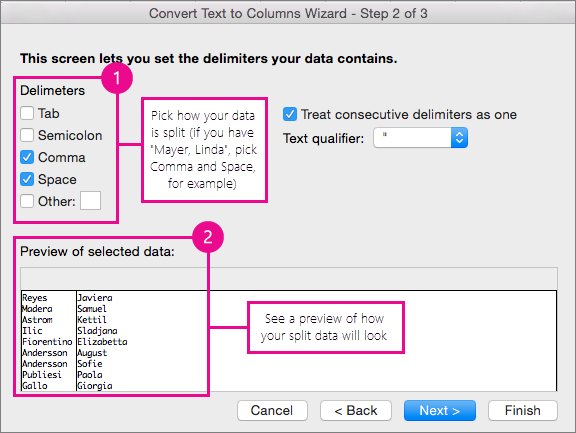
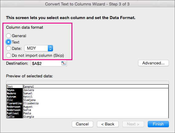
 button to the right of the Destination box to collapse the popup window.
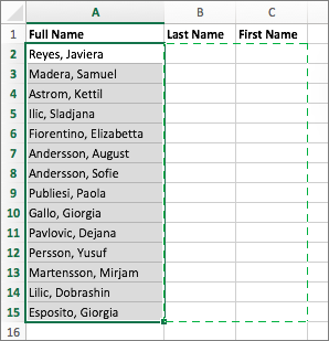
 button to expand the popup window again, and then click the Finish button.
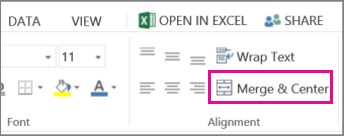
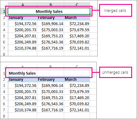
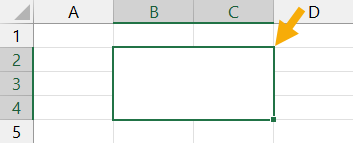


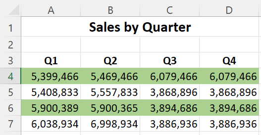

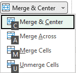
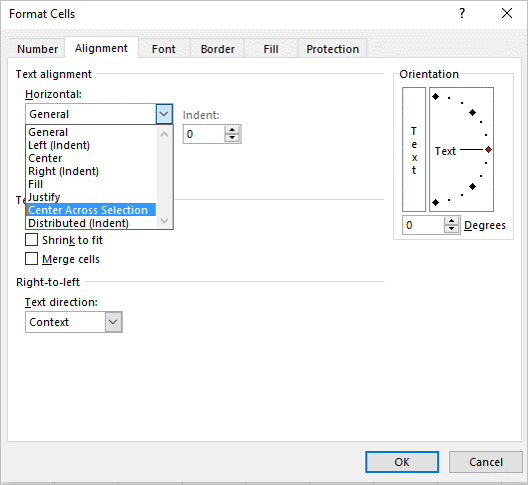


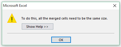
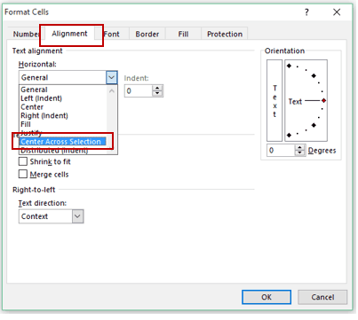

![Download 10 Excel Templates for Marketers [Free Kit]](https://no-cache.hubspot.com/cta/default/53/9ff7a4fe-5293-496c-acca-566bc6e73f42.png)
