Combine the MAX and IF functions in an array formula
Updated on March 26, 2020
The MAX IF array formula searches for the maximum value based on specific criteria. In the example below, we use MAX IF to find the best (highest) result for two track and field events – the high jump and pole vault – just by changing the search criterion.
These instructions apply to Microsoft Excel for Microsoft 365 and Excel 2019, 2016, 2010, and 2007.
CSE Formulas
You create array formulas by pressing the Ctrl, Shift, and Enter keys on the keyboard in succession once you’ve typed in the formula.
Because of the keys pressed to create the array formula, people sometimes call them CSE formulas.
MAX IF Nested Formula Syntax and Arguments
The job of each part of the formula is:
- The MAX function finds the highest result for the event chosen.
- The IF function allows us to choose the event by setting a condition using the event names.
- The array formula lets the IF function test for multiple conditions in a single cell, and, when the data meets a condition, the array formula determines what data (event results) the MAX function will examine to find the best result.
The syntax for the MAX IF formula is:
- Since the IF function nests inside the MAX function, the entire IF function becomes the sole argument for the MAX function.
The arguments for the IF function are:
- logical_test (required): A value or expression that is tested to see if it is true or false.
- value_if_true (required) The value that is displayed if logical_test is true.
- value_if_false (optional) The value that is displayed if logical_test is false.
In this example:
- The logical test tries to find a match for the event name typed into cell D10 of the worksheet.
- The value_if_true argument will be, with the help of the MAX function, the best result for the chosen event.
- The value_if_false argument isn’t necessary in this case, and its absence will shorten the formula. If an event name that is not in the data table — such as the long jump — is typed into cell D10 it will return a zero (0).
Entering the MAX IF Nested Formula
The job of each part of the formula is:
- The MAX function finds the highest result for the event chosen.
- The IF function allows us to choose the event by setting a condition using the event names.
- The array formula lets the IF function test for multiple conditions in a single cell, and, when the data meets a condition, the array formula determines what data (event results) the MAX function will examine to find the best result.
Since we are creating both a nested formula and an array formula, we will need to type it directly into a worksheet cell.
Once you have entered the formula, do not press the Enter key on the keyboard or click on a different cell with the mouse as we need to turn the formula into an array formula.
-
Enter the following data into cells D1 to E9 as seen in this image.
-
Type high jump into cell D10. The formula will look at this cell to match it with the events in cells D2 to D7.
-
Select cell E10 which is the location where the formula results will be displayed.
-
Type the following:
=MAX( IF(D2:D7=D10, E2:E7) )
-
Press the Enter key on the keyboard to create the array formula.
-
Test the formula by finding the best result for the pole vault. Type pole vault into cell D10 and press the Enter key on the keyboard. The formula should return the height of 5.65 meters in cell E10.
Thanks for letting us know!
Get the Latest Tech News Delivered Every Day
Subscribe

Иногда вместо того, чтобы просто найти наибольшее или максимальное число для всех ваших данных; вам нужно найти наибольшее число в подмножестве — например, наибольшее положительное или отрицательное число.
Если объем данных небольшой, задачу можно легко выполнить, вручную выбрав правильный диапазон для функции MAX .
В других обстоятельствах, таких как большая выборка несортированных данных, правильный выбор диапазона может оказаться трудным, если не невозможным.
Комбинируя функцию IF с MAX в формуле массива , можно легко установить условия, такие как только положительные или отрицательные числа, чтобы по формуле проверялись только данные, соответствующие этим параметрам.
MAX IF Разбивка формулы массива
Формула, используемая в этом руководстве, чтобы найти наибольшее положительное число:
= МАКС. (ЕСЛИ (A1: B5> 0, A1: B5))
Аргумент value_if_false функции IF, который является необязательным, опущен, чтобы сократить формулу. Если данные в выбранном диапазоне не соответствуют установленному критерию — числа больше нуля — формула вернет ноль (0)
Работа каждой части формулы:
- Функция IF фильтрует данные так, что только те числа, которые соответствуют выбранному критерию, передаются в функцию MAX
- функция MAX находит наибольшее значение для отфильтрованных данных
- Формула массива, обозначенная фигурными скобками {}, окружающими формулу, позволяет логическому тестовому аргументу функции IF выполнять поиск во всем диапазоне данных на предмет совпадения, например, числа больше нуля, а не только в одной ячейке данных.
CSE Формулы
Формулы массива создаются одновременным нажатием клавиш Ctrl , Shift и Enter на клавиатуре после ввода формулы.
В результате вся формула, включая знак равенства, окружена фигурными скобками. Примером может быть:
{= МАКС. (ЕСЛИ (A1: B5> 0, A1: B5))}
Из-за клавиш, нажимаемых для создания формулы массива, их иногда называют формулами CSE .
Пример формулы MAX IF Array для Excel
Шаги ниже сначала создают формулу, чтобы найти наибольшее положительное число, затем следуют шаги, необходимые для поиска наибольшего отрицательного числа.
Ввод данных учебника
- Введите числа, показанные на рисунке выше, в ячейки от А1 до В5 рабочего листа.
- В ячейках A6 и A7 введите метки Max Positive и Max Negative.
Ввод MAX IF вложенной формулы
После того, как вы ввели формулу, НЕ нажимайте клавишу Enter на клавиатуре или щелкайте мышью по другой ячейке, поскольку нам нужно превратить формулу в формулу массива.
- Нажмите на ячейку B6 — место, где будут отображаться результаты первой формулы
- Введите следующее:
= МАКС. (ЕСЛИ (A1: B5> 0, A1: B5))
Создание формулы массива
- Нажмите и удерживайте клавиши Ctrl и Shift на клавиатуре
- Нажмите клавишу Enter на клавиатуре, чтобы создать формулу массива
- Ответ 45 должен появиться в ячейке B6, так как это самое большое положительное число в списке
{= МАКС. (ЕСЛИ (A1: B5> 0, A1: B5))}
Нахождение наибольшего отрицательного числа
Поскольку теперь цель состоит в том, чтобы найти наибольшее отрицательное число, вторая формула использует оператор меньше чем ( < ), а не больше, чем оператор ( > ), чтобы проверить только те данные, которые меньше нуля.
- Нажмите на ячейку B7
- Введите следующее:
= МАКС. (ЕСЛИ (A1: B5 <0, A1: B5))
- Выполните шаги выше, чтобы создать формулу массива
- Ответ -8 должен появиться в ячейке B7, так как это самое большое отрицательное число в списке
The example shown contains almost 10,000 rows of data. The data represents temperature readings taken every 2 minutes over a period of days. For any given date (provided in cell H7), we want to get the maximum temperature on that date.
Inside the IF function, logical test is entered as B5:B9391=H7. Because we’re comparing the value in H7 against a range of cells (an array), the result will be an array of results, where each item in the array is either TRUE or FALSE. The TRUE values represent dates that match H7.
For the value if true, we provide the range E5:E9391, which fetches all the full set of temperatures in Fahrenheit. This returns an array of values the same size as the first array.
The IF function acts as a filter. Because we provide IF with an array for the logical test, IF returns an array of results. Where the date matches H7, the array contains a temperature value. In all other cases, the array contains FALSE. In other words, only temperatures associated with the date in H7 survive the trip through the IF function.
The array result from the IF function is delivered directly to the MAX function, which returns the maximum value in the array.
With MAXIFS
In Excel O365 and Excel 2019, the new MAXIFS function can find the maximum value with one or more criteria without the need for an array formula. With MAXIFS, the equivalent formula for the this example is:
=MAXIFS(E5:E9391,B5:B9391,H7)
Excel MAX IF Function (Table of Contents)
- MAX IF in Excel
- How to Use MAX IF Function in Excel?
MAX IF in Excel
Max function and IF function in Excel are used to find the maximum value from the given range of datasets with the defined criteria. The MAX function returns the maximum value from the select number range, and the IF function helps find that number with chosen criteria. For this, we can first apply the IF function where, as per syntax, first choose Criteria Range and with the criteria we want, then select the value range. Once done, then cover the complete IF function in the MAX function’s syntax with curly brackets.
In Microsoft Excel, there is no such separate syntax for the MAXIF function, but we can combine the MAX and IF function in an array formula.
MAX Formula in Excel
Below is the MAX Formula in Excel:
Arguments of MAX Formula:
- number1: This number1 refers to a numeric value or range which contains a numeric value.
- number2 [optional]: This number2 refers to a numeric value or range which contains a numeric value.
IF Formula in Excel
Below is the IF Formula in Excel:
Arguments of IF Formula:
- Logical test: Which is a logical expression value to check the value is TRUE or FALSE.
- value _if_ true: Which is a value that returns if the logical test is true.
- value _if_ false: Which is a value that returns if the logical test is false.
How to Use MAX IF Function in Excel?
MAX and IF Functions in Excel is very simple and easy to use. Let’s understand the working of the MAX IF Function in Excel with some example.
You can download this MAX IF Function Excel Template here – MAX IF Function Excel Template
Example #1 – MAX Function in Excel
In this example, we will first learn how to use the MAX function with the below example.
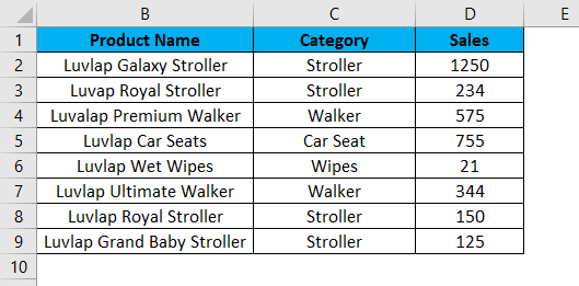
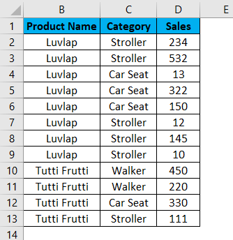
Consider the below example, which shows sales data of the product category wise.
Now we will use the MAX function to find out which has the largest sales value by following the below steps.
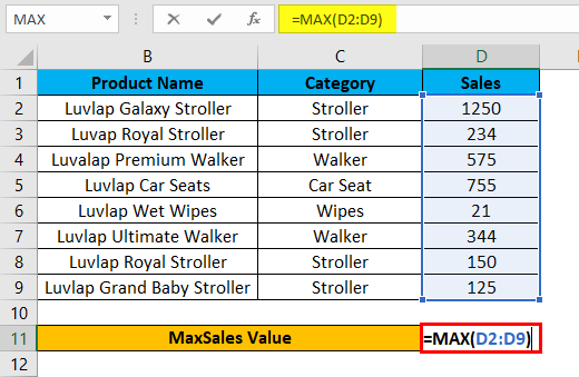
Step 1 – First, select the new cell, i.e. D11.
Step 2 – Apply the MAX function i.e. =MAX(D2:D9)
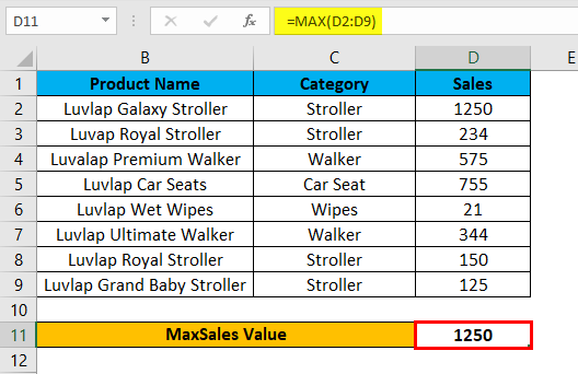
Step 3 – Press enter so that we will get the MAX value is 1250, which is shown in the below screenshot.
In the below result, the Max function will check for the largest number in the D column and return the maximum sales value as 1250.
Example #2 – Using MAX IF Function in Excel with an array formula
In this example, we will learn how to use MAX IF function in Excel. Assume that we need to check the largest sales value category wise. Using only the max function, we can check only the maximum value, but we cannot check the maximum value category wise if the sales data contain a huge category and sales value.
In such a case, we can combine MAX and If Function with an array formula so that it makes the task very easier to find out the largest sales value category wise in Excel.
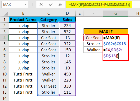
Consider the below example, which has Product Name, Category and Sales value which is shown below.
Now we will apply the Excel MAX IF function to find out the maximum sales value by following the below steps.
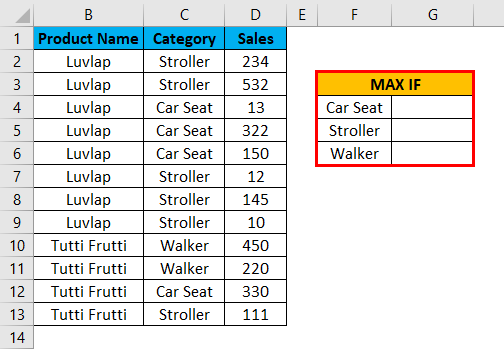
Step 1 – First, we will create a new table with a category name to display the result, as shown below.
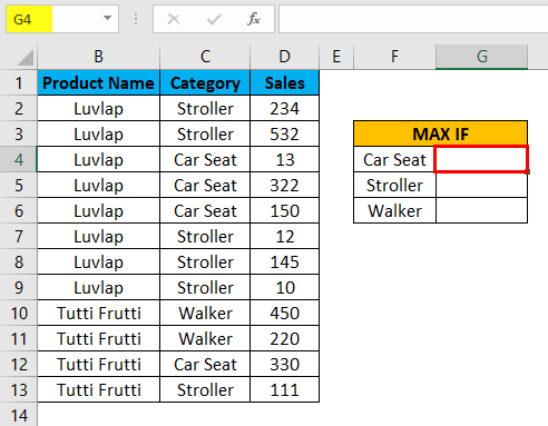
Step 2 – Select cell G4.
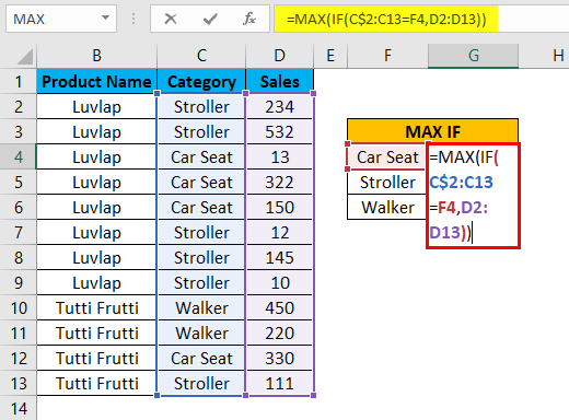
Step 3 – Apply the MAX IF formula i.e. =MAX(IF(C$2:C13=F4,D2:D13))
In the above formula, we have applied MAX and IF function and then we selected Column C2 to C13 where we have listed the category name as C2:C13 and then we have checked the condition by selecting the cell as F4 where the F4 column is nothing but Category Name.
Now the if condition will check for the entire category name in C2 to C13 column whether it matches with the mentioned Category name in the F4 column; if the category name matches, it will return the largest sales value from the selected D column as D2 to D13 and lock the cells by pressing F4 where we will get the $ symbol to indicate that cells are locked, and we have given the Formula as =MAX(IF($C$2:$C$13=F4,$D$2:$D$13)).
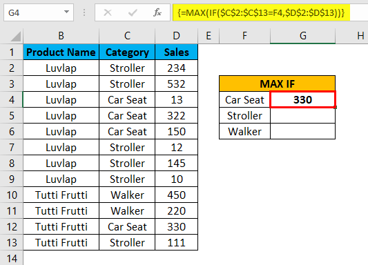
After the MAXIF function is completed by closing all the brackets now, hold SHIFT+CTRL and then press enter as SHIFT+CTRL+ENTER so that we will get the output in array formula where we will get open and closing parenthesis at the opening and end of the statement, which is shown in the below screenshot.
Here as we can see in the above screenshot MAX IF function check for the category name in the D column as well as in the F column, and if it matches, it will return the largest value; here in this example, we got the output as 330 which is a largest sales value in the category.
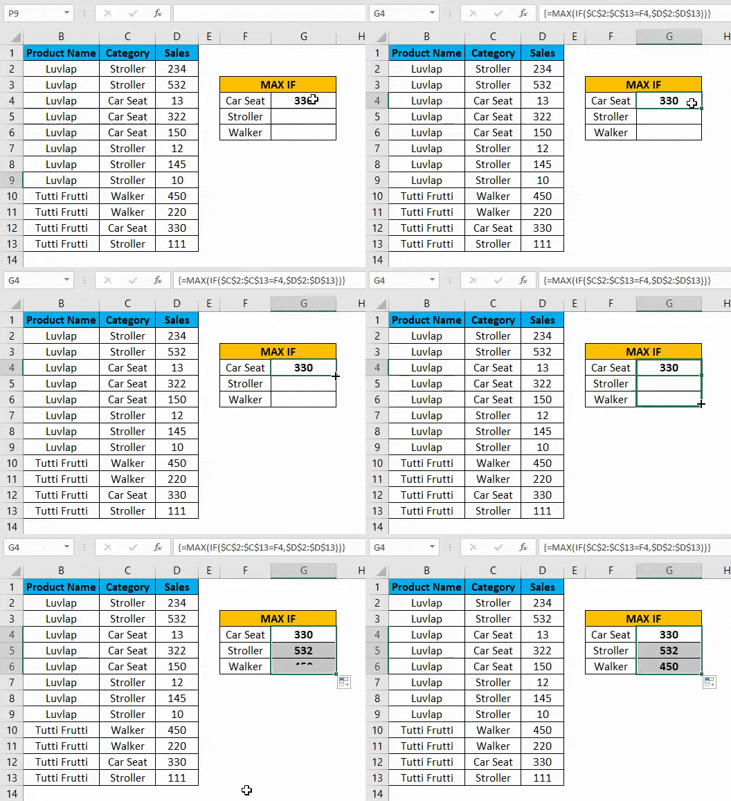
Now drag down the MAX IF formulas for all the cell so that we will get the output result which is shown below.
Example #3 – Using MAX IF Function in Excel with an array formula
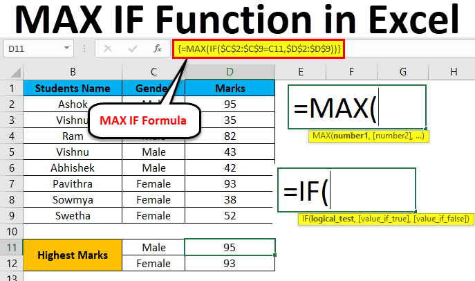
In this example, we will use the same Excel MAX IF function to find out the highest marks from a set of students.
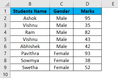
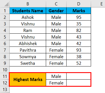
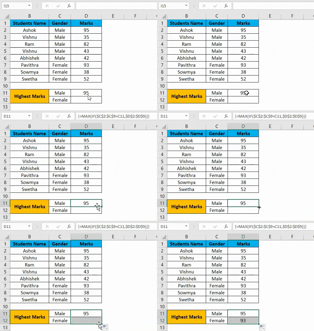
Consider the below example, which shows student name along with their Gender and Marks, which is shown below.
Here in this example, we are going to find out Gender wise who has scored the highest marks by following the below steps.
Step 1 – First, create a new table with Male and Female as a separate column to display the result, which is shown below.
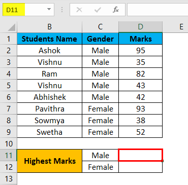
Step 2 – Now, we will apply the Excel MAX IF function as follows. Select cell D11.
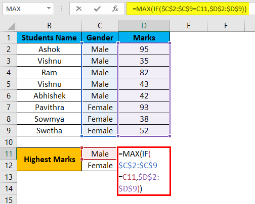
Step 3 – Insert the MAX IF function by selecting the Gender column from C2 to C9.
Now we have to give the condition as IF(C2:C9=C11,D2:D9), which means that the IF condition will check for the gender from the C2 column whether it matches with C11 and If the gender matches MAX IF function returns the highest value.
Step 4 – Now lock the cells by pressing F4 so that the selected cells will be locked, which is shown in the below screenshot.
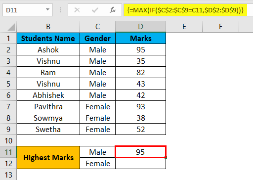
Step 5 – Once we complete the MAXIF function, Hit SHIFT+CRL+ENTER to make it an array formula to see the opening and closing parenthesis in the MAX IF function, which is shown below.
We can see that we got the highest mark as 95 for the gender MALE in the above screenshot.
Step 6 – Drag down the formula for all the below cells so that we will get the output as shown below.
In the above result using the Excel MAX IF function, we have found the highest marks gender-wise where MALE has scored 95 as the highest mark, and for FEMALE, we got 93 as the Highest mark.
Things to Remember
- In Microsoft Excel, there is no such MAX IF function as SUMIF and COUNTIF.
- We can use the MAX and IF function by combining them in the formulation.
- MAX IF function will throw an error #VALUE! If we did not apply the SHIFT+ENTER +KEY, make sure that you are using MAX IF function as an array formula.
Recommended Articles
This has been a guide to MAX IF in Excel. Here we discuss how to use MAX IF Function in Excel along with practical examples and downloadable excel templates. You can also go through our other suggested articles –
- MAX Excel Function
- SUMIF in Excel
- Excel SUM MAX MIN AVERAGE
- MAX Formula in Excel
In Excel, we can’t simply use the default MAX function with a condition (unless you are using Microsoft Office 365).
But the thing is if want to get maximum value from a range using a specific condition you need a MAX IF formula.
So what’s the point?
You can combine MAX and IF to create a formula that can help you to get the max value from a range using specific criteria.
In short: MAXIF is an array formula that you can use to find the max value from a range using criteria. But here’s the kicker: In this post, I’m gonna share with you different ways to use the MAXIF formula.
Apply MAX IF Formula
Let’s take an example of the below data where you have month-wise, week-wise, and date-wise sales quantity.

Now from this data, you need to get the max sales quantity for a particular month. For example, “Jan” and for this, the formula will be:
=MAX(IF(A2:A367="Jan",D2:D367))And you need to enter it as an array formula by using ctrl + shift + enter.
{=MAX(IF(A2:A367="Jan",D2:D367))}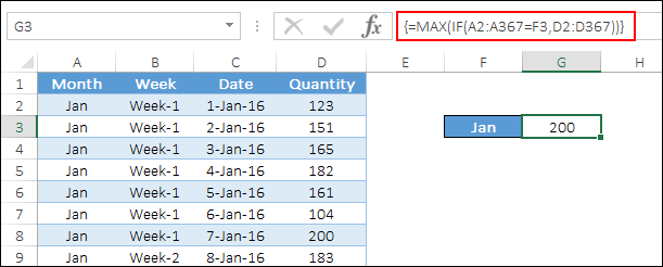
When you enter it, it will return 200 which is the highest sales value in the month of Jan on 07-Jan-2016.
How does this work
To understand the working of max if you need to split it into three parts.

Please take note that you have entered it as an array formula.
First of all, you have created a logical test in the IF function to match the entire month column with the criteria. And, it has returned an array where match values are TRUE and all others are FALSE.

Second, in the IF function, you have specified the sales quantity column for the TRUE values and that’s why it has returned sales quantity only for the TRUE.

Third, the MAX function will simply return the highest number from this array which is the highest sales quantity for the month of Jan. Just like this formula hack here I’ve listed some of the others which you must read and learn.
- SUMIFOR in Excel
- RANKIF in Excel
I am sure at this point you are thinking that how we can use more than one condition in max if. And that’s a smart thought.
In the real world of data, there is a huge possibility that we need to use multiple criteria to get the highest value. Let’s continue with the previous example.
Let’s say, instead of the highest sales value from the month of Jan, you need to get the highest sales for week 2 of Jan.
So, here you have two different conditions, the month is Jan and the week is the 2nd. And, the formula will be:
=MAX(IF(A2:A367=F5,IF(B2:B367=G5,D2:D367),))And, when you enter it as an array:
{=MAX(IF(A2:A367=F5,IF(B2:B367=G5,D2:D367),))}
How does this work
Here we have used nested IF to test more than one logic. One is for the month and the second is for the week.
So it returns an array where you have sales quantity only where the month is Jan and the week is the 2nd.

And in the end, max returns the max value from that array.
MAX IF without an Array
Arrays are powerful but not everyone wants to use them. And, you have an option not to use an array in max if.
So for this, you can use the SUMPRODUCT function because it can help you to use an array without applying the actual array formula. And the formula will be:
=SUMPRODUCT(MAX((A2:A367="Jan")*D2:D367))So when you insert this formula you don’t need to use ctrl + shift + enter.
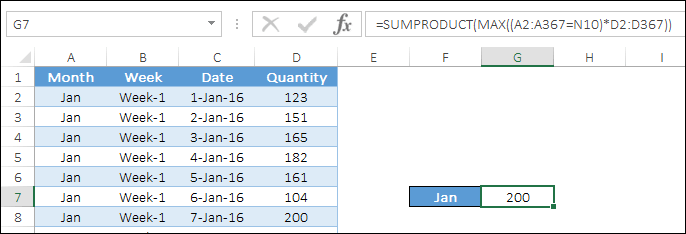
How does this work
Again we need to split this formula into three different parts to understand it. In the first part, you have compared the month column with the criteria and it has returned an array with TRUE where criteria matched, else FALSE.

After that, you have multiplied that array with the sales quantity column which returns an array where you have sales quantity instead of TRUE. In the end, the MAX function has returned the highest value from that array which is your highest sales quantity.
This entire formula, sumproduct has the major role to allow you to use an array without entering an actual array formula.
Conclusion
Getting the max value based on criteria is what we often need to do. And using this technique of max if the formula you can do it with no effort.
All the methods which you have learned above have different applications according to the situation. I hope this formula tip will help you to get better at Excel. But now, tell me one thing.
Which one do you really like, an array or without an array?
Please share your views with me in the comment section. I’d love to hear from you, and please, don’t forget to share this post with your friends, I am sure they will appreciate it.

