
To find the maximum date in Excel with a condition, you will need to use the MAXIFS function. MAXIFS works the same way as the MAX function, but you can use a criteria to determine which cells are included in the calculation.
For example, suppose you have a range of dates in column A and a corresponding value in column B, and you want to find the maximum of column B where the dates in column A are in the same month. In this case, you could write the following formula:
=MAXIFS(B:B,A:A,”>=FirstDayOfMonth”,A:A,”
Replace FirstDayOfMonth and LastDayOfMonth with the corresponding dates for the month you are referring to. This formula will then return the highest corresponding value for that month in column B.
You can use this same approach to find other maximum values with conditions, such as the highest value in a range where the corresponding text in a certain column starts with a certain letter. You just need to adjust the criteria accordingly.
Hopefully this has explained how to use MAXIFS to find the maximum date with a condition!
How do you use Max function in Excel with multiple conditions?
The Max function in Excel can be used with multiple conditions in order to return the maximum of all selected values. To do this, you need to start by creating a formula with the Max function and setting two conditions: one condition for the values you want to analyze, and one condition for the maximum value you want to return.
For example, to find the maximum of two values (1,2), you would use the following formula: =MAX(IF(A1:B2=1,1,2)). This formula will return either 1 or 2 as the maximum value, depending on which value is larger.
You can also use the Max function with more than two conditions. To do this, you need to use the IF statement nested within the Max function in order to set multiple conditions. For example, to find the maximum of three values (1,2,3), you would use the following formula: =MAX(IF(A1:B3=1,1,IF(A1:B3=2,2,3))).
This formula will return either 1, 2, or 3 as the maximum value, depending on which value is the largest.
The Max function with multiple conditions can be used to quickly find the maximum value among a range of values. It is a invaluable tool for data analysis in Excel.
How do I combine an if and max in Excel?
In Microsoft Excel, it is possible to combine the use of an “IF” and “MAX” formula. This can be useful when you need to find the maximum value that meets certain criteria. To do this, you will first need to enter your data into the worksheet.
Make sure that the data is organized in its own column.
Next, click the cell where you want the maximum value to be displayed. In this cell, you will enter the following formula: =MAX(IF(logical_test,value_if_true,value_if_false)). This formula has three parts: logical_test, value_if_true, and value_if_false.
For logical_test, you will enter a comparison statement such as A1>5. This statement will determine which values from the data should be used to help find the maximum value.
For value_if_true, you will enter the cell range for the column of data that you want to evaluate for the maximum value.
For value_if_false, you will enter 0 as this part of the formula should only return a value of zero for cells that don’t meet the criteria set by the logical_test.
Once you have entered the formula, press Enter and the maximum value that meets your criteria will appear.
What is Max function in Excel with example?
The Max function in Excel is used to find the maximum value in a range of cells or numbers. For example, if you have a range of numbers in cells A2 through A10 and you wish to know the highest number, you would use the Max function.
In this instance, the syntax of the Max function would be =MAX(A2:A10). When the Max function is used Excel will scan the range of cells and return the highest value from the range. The function can also be used on multiple ranges of cells.
For example, to find the maximum value from multiple ranges of cells such as A2:A10 and B2:B10 you would use the syntax: =MAX(A2:A10,B2:B10). Again, Excel will scan both ranges of cells to return the highest value.
Can we use Max on date?
Yes, Max can be used on date. Max is a command-line program that can search and analyze data in text files. It is most commonly used to parse large amounts of data quickly and efficiently and can be used on a variety of data including dates.
Max is capable of recognizing and sorting dates in a variety of formats including ISO8601 and Unix Epoch, and it can also manipulate dates by using different functions to calculate the difference between dates, convert timestamps, or subtract dates.
For example, the max command “max -s ‘date’” can be used to search text files for any dates in ISO8601 format and output them to the terminal. Additionally, Max can perform arithmetic functions on date data, such as calculating the number of days between two dates or adding days to a date.
Max also provides helpful functions like searching for the latest date in a series of timestamps and sorting dates in ascending or descending order. By using Max on date data, users can quickly parse and analyze large amounts of data and make more informed decisions.
How do I pull a date range in Excel?
To pull a date range in Excel, follow these steps:
1. Start by entering your date range into the first two rows of your Excel worksheet. Place the starting date of the range in the first cell, and the ending date of the range in the second cell.
2. Select both cells by clicking and dragging your mouse.
3. Go to the ‘Home’ tab, then select ‘Fill’ followed by ‘Series’.
4. The ‘Series’ dialogue box will then open. Make sure ‘Columns’ is selected and that the ‘Type’ option is set to ‘Date’.
5. Choose the ‘Date Unit’ from the drop-down list (e.g. months).
6. Click the ‘OK’ button and the dates within your selected range will automatically appear in the cells between your start and end dates.
What is the formula of maximum?
The formula for the maximum of a set of numbers is the largest value that exists in the set. To calculate the maximum of a set of numbers, you will first need to arrange the numbers in descending order.
Once they are in descending order, you will then select the first number in the list as it is the largest of the set and this is the maximum value of the set.
What is the max value for TIMESTAMP?
The maximum value for a TIMESTAMP data type is ‘9999-12-31 23:59:59’, which resolves to the year 10,000. This value is the maximum value that can be represented using the TIMESTAMP data type. The actual maximum range of the TIMESTAMP depends on the system used, as some implementations of it may have a limit of 9999-12-31 23:59:59 or even earlier year values such as 2038-01-19 03:14:07.
This means that the maximum value is dependent on the system used.
Is there a TIMESTAMP function in Excel?
Yes, there is a TIMESTAMP function in Excel. This function is used to convert a date value or expression into a timestamp value. It takes two arguments: the date value or expression and the specific time value or expression.
The TIMESTAMP function returns a unique number which can be used to represent a specific moment in time. This can be useful in a variety of scenarios such as creating a unique identifier for a transaction log or capturing the time when a specific event happens, such as when a user’s data is changed.
The TIMESTAMP function can be found in the Date & Time category in the Functions library of Excel.
How do you calculate TIMESTAMP time?
Time stamp is a sequence of characters or encoded information which marks the point in time when something has occurred. It is typically used to synchronize data between two different systems or record when a data item was last changed.
To calculate time stamp time, you will need to convert a moment in time (such as a date, time and/or seconds) into a specific numerical representation. This is typically done by breaking the moment down into its components (such as minutes, seconds, days, etc.
) and then encoding it into a format that is easy to compare and interpret. For instance, the Unix Epoch Timestamp is a common time stamp format which represents the number of seconds that have passed since 00:00:00 UTC on January 1st, 1970.
To calculate this timestamp, you would need to subtract the Unix Epoch Timestamp from the current time represented in a universal format (such as UTC or GMT). Additionally, you can also calculate time stamps for specific moments in time (such as the start of a particular day, the beginning or end of a month, etc.
) by subtracting the desired point in time from the Unix Epoch Timestamp.
How do I get the latest date in VLOOKUP?
Using VLOOKUP to get the latest date is a bit more complicated than other uses of the formula because you must use two criteria—the first being to identify the correct row of data and the second being to identify the latest date in the row.
To do this, you must first format your data table to arrange the dates in chronological order. You can then use a combination of the INDEX, MATCH, and MAX functions to pull the latest date from your data table.
The INDEX function is used to pull the value from a cell in the data range; MATCH will identify the row of the latest date; and MAX will find the greatest value, which in our case is the latest date.
The combination works like this: INDEX(data table,MATCH(MAX(date column within data table),date column within data table,0)).
Assuming the dates are in column A and the data range is B1:D5, the formula would be:
INDEX(B1:D5,MATCH(MAX(A1:A5),A1:A5,0))
This formula willpull the latest date from the data table. It’s important to remember that this formula requires that your data table is properly arranged with the latest date at the top. Additionally, the latest date can only be pulled when the formula is entered into a cell in a different column.
Can you use VLOOKUP to retrieve dates?
Yes, you can use VLOOKUP to retrieve dates. VLOOKUP is a spreadsheet function that can be used to search for a specific value in a range of columns and return a related value from an adjacent column.
For example, if you have a list of dates stored in the first column of a spreadsheet and need to find a specific date and return the value located next to it, VLOOKUP can be used to do this. To do this, simply enter the date you are looking for in the first parameter of VLOOKUP and the range of columns that contain the dates as the second parameter.
The third parameter should be set to “TRUE” so that VLOOKUP will look for an exact match of the date given. The last parameter should be set to the column number of the adjacent cell that you want to return.
The VLOOKUP function can then be used to retrieve dates from the spreadsheet.
What does F4 in VLOOKUP do?
F4 in VLOOKUP is a shortcut that references the current cell when used in a formula. It’s used to ensure that the formula will refer to the same cell when the formula is copied to other cells. The reference points to the active cell, rather than an absolute cell reference.
This makes it easy to copy formulas without having to manually change the cell references each time. F4 can also be used in other functions, such as SUM, AVERAGE, or COUNT to reference multiple cells with a single formula.
How do you pull data from one Excel sheet to another based on date?
To pull data from one Excel sheet to another based on date, you can use a combination of several functions. First, you can use INDEX and MATCH functions to pull values from the source sheet. The MATCH function will be used to identify the row number of the date column on the source sheet, while the INDEX function will match that found row number with the corresponding value in the desired column.
Once you have the value you want, you can use the VLOOKUP function to copy it to the destination sheet. VLOOKUP will look up the date in the destination sheet and match it with the corresponding value on the source sheet.
You would need to ensure that the range in which VLOOKUP examines the source data is properly configured.
Overall, pulling data from one Excel sheet to another based on date is possible through the proper use of functions. It is important to understand the syntax of the functions involved, such as INDEX, MATCH, and VLOOKUP, in order to obtain the desired results.
Содержание
- Формула Excel MAX IF, чтобы найти наибольшее значение с условиями
- Формула Excel МАКС ЕСЛИ
- Как работает эта формула
- Формула MAX IF с несколькими критериями
- Как работают эти формулы
- МАКС. ЕСЛИ без массива
- Как работает эта формула
- Формула Excel MAX IF с логикой ИЛИ
- Как работают эти формулы
- MAXIFS — простой способ найти максимальное значение с условиями
- Max IF While Filtering dates?
- 1 Answer 1
- Max IF in Excel
- What is MAX IF Formula in Excel?
- How to use Max If Formula in Excel?
- The Cautions While Using MAX IF Formula
- Applications of Excel Max IF Formula
- Frequently Asked Questions
- Key Takeaways
- Recommended Articles
Формула Excel MAX IF, чтобы найти наибольшее значение с условиями
В статье показано несколько различных способов получить максимальное значение в Excel на основе одного или нескольких указанных вами условий.
В нашем предыдущем руководстве мы рассмотрели распространенное использование функции MAX, которая предназначена для возврата наибольшего числа в наборе данных. Однако в некоторых ситуациях вам может потребоваться углубиться в свои данные, чтобы найти максимальное значение на основе определенных критериев. Это можно сделать с помощью нескольких различных формул, и в этой статье объясняются все возможные способы.
Формула Excel МАКС ЕСЛИ
До недавнего времени в Microsoft Excel не было встроенной функции МАКС. ЕСЛИ для получения максимального значения в зависимости от условий. С введением MAXIFS в Excel 2019 мы можем легко выполнять условное максимальное значение.
В Excel 2016 и более ранних версиях вам все равно придется создавать собственную формулу массива, комбинируя функцию MAX с оператором IF:
<=МАКС(ЕСЛИ(критерии_диапазонзнак равнокритерии, максимальный_диапазон))>
Чтобы увидеть, как эта общая формула MAX IF работает с реальными данными, рассмотрим следующий пример. Предположим, у вас есть таблица с результатами прыжков в длину нескольких учеников. В таблицу включены данные по трем раундам, и вы ищете лучший результат конкретного спортсмена, скажем Якова. С именами учащихся в A2:A10 и расстояниями в C2:C10 формула принимает следующий вид:
Помните, что формулу массива всегда нужно вводить, одновременно нажимая клавиши Ctrl + Shift + Enter. В результате он автоматически обрамляется фигурными скобками, как показано на скриншоте ниже (набор фигурных скобок вручную не работает!).
В реальных рабочих листах критерий удобнее вводить в какую-то ячейку, чтобы можно было легко изменить условие, не меняя формулу. Итак, набираем нужное имя в F1 и получаем следующий результат:
=МАКС(ЕСЛИ(A2:A10=F1, C2:C10))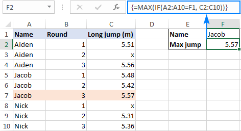
Как работает эта формула
В логическом тесте функции ЕСЛИ мы сравниваем список имен (A2:A10) с целевым именем (F1). Результатом этой операции является массив значений ИСТИНА и ЛОЖЬ, где значения ИСТИНА представляют имена, совпадающие с целевым именем (Джейкоб):
Для значение_ если_истина аргумент, мы предоставляем результаты длинного перехода (C2:C10), поэтому, если логический тест оценивается как TRUE, возвращается соответствующее число из столбца C. значение_ если_ложь аргумент опущен, то есть будет иметь значение FALSE, если условие не выполняется:
Этот массив передается функции MAX, которая возвращает максимальное число, игнорируя значения FALSE.
Кончик. Чтобы просмотреть внутренние массивы, описанные выше, выберите соответствующую часть формулы на листе и нажмите клавишу F9. Чтобы выйти из режима оценки формулы, нажмите клавишу Esc.
Формула MAX IF с несколькими критериями
В ситуации, когда вам нужно найти максимальное значение на основе более чем одного условия, вы можете:
Используйте вложенные операторы IF, чтобы включить дополнительные критерии:
<=МАКС(ЕСЛИ(критерии_диапазон1знак равнокритерии1ЕСЛИ(критерии_диапазон2знак равнокритерии2, максимальный_диапазон)))>
Или обработайте несколько критериев, используя операцию умножения:
<=МАКС(ЕСЛИ((критерии_диапазон1знак равнокритерии1) * (критерии_диапазон2знак равнокритерии2), максимальный_диапазон))>
Допустим, у вас есть результаты юношей и девушек в одной таблице и вы хотите найти самый длинный прыжок среди девушек в 3 туре. Для этого вводим первый критерий (женский) в G1, второй критерий (3) в G2 и используйте следующие формулы для определения максимального значения:
=МАКС(ЕСЛИ(B2:B16=G1, ЕСЛИ(C2:C16=G2, D2:D16)))
Поскольку обе формулы являются формулами массива, не забудьте нажать Ctrl + Shift + Enter, чтобы заполнить их правильно.
Как показано на снимке экрана ниже, формулы дают одинаковый результат, поэтому какую из них использовать, зависит от ваших личных предпочтений. Для меня формулу с булевой логикой легче читать и строить — она позволяет добавлять сколько угодно условий без вложения дополнительных функций ЕСЛИ.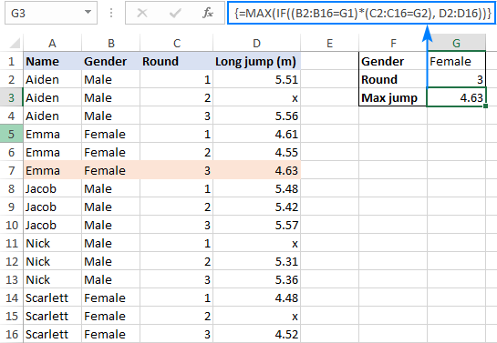
Как работают эти формулы
Первая формула использует две вложенные функции ЕСЛИ для оценки двух критериев. В логической проверке первого оператора IF мы сравниваем значения в столбце «Пол» (B2:B16) с критерием в G1 («Женский»). Результатом является массив значений TRUE и FALSE, где TRUE представляет данные, соответствующие критерию:
Аналогичным образом вторая функция ЕСЛИ проверяет значения в столбце округления (C2:C16) на соответствие критерию в G2.
Для значение_если_истина аргумент во втором операторе IF, мы предоставляем результаты прыжка в длину (D2:D16), и таким образом мы получаем элементы, которые имеют TRUE в первых двух массивах в соответствующих позициях (т. е. элементы, где пол «женский» и круглые равно 3):
Этот последний массив передается функции MAX, и она возвращает наибольшее число.
Вторая формула оценивает одни и те же условия в рамках одного логического теста, а операция умножения работает как оператор И:
Когда значения TRUE и FALSE используются в любой арифметической операции, они преобразуются в 1 и 0 соответственно. А поскольку умножение на 0 всегда дает ноль, результирующий массив имеет 1 только тогда, когда все условия ИСТИННЫ. Этот массив оценивается в логической проверке функции ЕСЛИ, которая возвращает расстояния, соответствующие элементам 1 (ИСТИНА).
МАКС. ЕСЛИ без массива
Многие пользователи Excel, в том числе и я, предвзято относятся к формулам массивов и стараются по возможности избавиться от них. К счастью, в Microsoft Excel есть несколько функций, которые изначально обрабатывают массивы, и мы можем использовать одну из таких функций, а именно СУММПРОИЗВ, как своего рода «оболочку» вокруг MAX.
Общая формула MAX IF без массива выглядит следующим образом:
=СУММПРОИЗВ(МАКС((критерии_диапазон1знак равнокритерии1) * (критерии_диапазон2знак равнокритерии2) * максимальный_диапазон))
Естественно, при необходимости вы можете добавить больше пар диапазон/критерий.
Чтобы увидеть формулу в действии, мы будем использовать данные из предыдущего примера. Цель состоит в том, чтобы получить максимальный прыжок спортсменки в раунде 3:
=СУММПРОИЗВ(МАКС(((B2:B16=G1) * (C2:C16=G2) * (D2:D16))))
Эта формула заменяется обычным нажатием клавиши Enter и возвращает тот же результат, что и формула массива MAX IF:
Присмотревшись к приведенному выше снимку экрана, вы можете заметить, что недопустимые переходы, отмеченные знаком «x» в предыдущих примерах, теперь имеют 0 значений в строках 3, 11 и 15, и в следующем разделе объясняется, почему.
Как работает эта формула
Как и в случае с формулой МАКС. ЕСЛИ, мы оцениваем два критерия, сравнивая каждое значение в столбцах «Пол» (B2:B16) и «Округление» (C2:C16) с критериями в ячейках G1 и G2. Результатом являются два массива значений TRUE и FALSE. Умножение элементов массивов в одинаковых позициях преобразует ИСТИНА и ЛОЖЬ в 1 и 0 соответственно, где 1 представляет элементы, соответствующие обоим критериям. Третий умноженный массив содержит результаты прыжков в длину (D2:D16). И поскольку умножение на 0 дает ноль, выживают только элементы, имеющие 1 (ИСТИНА) в соответствующих позициях:
В случае максимальный_диапазон содержит любое текстовое значение, операция умножения возвращает ошибку #ЗНАЧ, из-за которой вся формула не работает.
Функция MAX берет его отсюда и возвращает наибольшее число, удовлетворяющее заданным условиям. Результирующий массив, состоящий из одного элемента <4.63>, поступает в функцию СУММПРОИЗВ и выводит максимальное число в ячейке.
Примечание. Из-за своей специфической логики формула работает со следующими оговорками:
- Диапазон, в котором вы ищете наибольшее значение, должен содержать только числа. Если есть какие-либо текстовые значения, #VALUE! возвращается ошибка.
- Формула не может оценить условие «не равно нулю» в отрицательном наборе данных. Чтобы найти максимальное значение без учета нулей, используйте либо формулу МАКС. ЕСЛИ, либо функцию МАКС.
Формула Excel MAX IF с логикой ИЛИ
Чтобы найти максимальное значение при выполнении любого из указанных условий, используйте уже знакомую формулу массива МАКС ЕСЛИ с булевой логикой, но сложите условия, а не перемножайте их.
<=МАКС(ЕСЛИ((критерии_диапазон1знак равнокритерии1) + (критерии_диапазон2знак равнокритерии2), максимальный_диапазон))>
Кроме того, вы можете использовать следующую формулу без массива:
=СУММПРОИЗВ(МАКС(((критерии_диапазон1знак равнокритерии1) + (критерии_диапазон2знак равнокритерии2)) * максимальный_диапазон))
Для примера вычислим лучший результат в раундах 2 и 3. Обратите внимание, что в языке Excel задача формулируется иначе: вернуть максимальное значение, если раунд либо 2, либо 3.
С раундами, перечисленными в B2:B10, результатами в C2:C10 и критериями в F1 и H1, формула выглядит следующим образом:
=МАКС(ЕСЛИ((B2:B10=F1) + (B2:B10=H1), C2:C10))
Введите формулу, нажав комбинацию клавиш Ctrl + Shift + Enter, и вы получите такой результат:
Максимальное значение с теми же условиями также можно найти с помощью этой формулы без массива:
=СУММПРОИЗВ(МАКС(((B2:B10=F1) + (B2:B10=H1)) * C2:C10))
Однако в этом случае нам нужно заменить все значения «x» в столбце C нулями, потому что СУММПРОИЗВ МАКС работает только с числовыми данными:
Как работают эти формулы
Формула массива работает точно так же, как МАКС. ЕСЛИ с логикой И за исключением того, что вы соединяете критерии, используя операцию сложения вместо умножения. В формулах массива сложение работает как оператор ИЛИ:
Сложение двух массивов ИСТИНА и ЛОЖЬ (которые получаются в результате проверки значений в B2:B10 по критериям в F1 и H1) дает массив из 1 и 0, где 1 представляет элементы, для которых любое условие является ИСТИННЫМ, а 0 представляет элементы. для которого оба условия ЛОЖНЫ. В результате функция ЕСЛИ «сохраняет» все элементы в C2:C10 (значение_если_истина), для которого любое условие ИСТИННО (1); остальные элементы заменяются на FALSE, потому что значение_если_ложь аргумент не указан.
Формула без массива работает аналогичным образом. Разница в том, что вместо логического теста IF вы умножаете элементы массива 1 и 0 на элементы массива результатов прыжка в длину (C2:C10) в соответствующих позициях. Это аннулирует элементы, которые не соответствуют ни одному условию (имеют 0 в первом массиве), и сохраняет элементы, которые соответствуют одному из условий (имеют 1 в первом массиве).
MAXIFS — простой способ найти максимальное значение с условиями
Пользователи Excel 2019, 2021 и Excel 365 избавлены от необходимости приручать массивы для создания собственной формулы MAX IF. Эти версии Excel предоставляют долгожданную функцию MAXIFS, которая упрощает поиск наибольшего значения в условиях детской игры.
В первом аргументе MAXIFS вы вводите диапазон, в котором должно быть найдено максимальное значение (в нашем случае D2:D16), а в последующих аргументах вы можете ввести до 126 пар диапазон/критерий. Например:
=МАКСЕСЛИ(D2:D16, B2:B16, G1, C2:C16, G2)
Как показано на снимке экрана ниже, у этой простой формулы нет проблем с обработкой диапазона, содержащего как числовые, так и текстовые значения: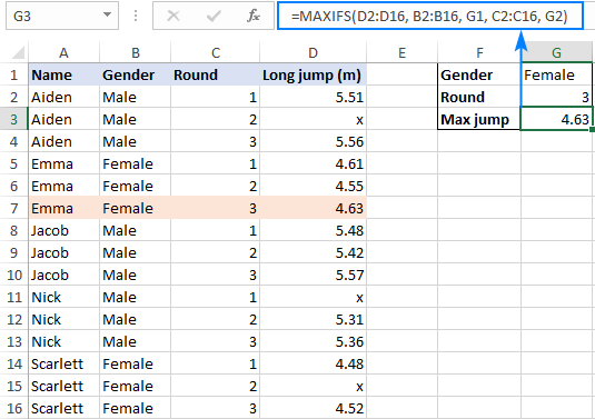
Подробную информацию об этой функции см. в разделе Функция MAXIFS в Excel с примерами формул.
Вот как вы можете найти максимальное значение с условиями в Excel. Я благодарю вас за чтение и надеюсь увидеть вас в нашем блоге на следующей неделе!
Источник
Max IF While Filtering dates?
How can I find the max date that is less than today in a range that is mixed with both ACTUAL and PROJECTED Dates: 
as you see here I have a row of dates. Some dates are actual, others are projected. I want to open the spreadsheet and say «What is the latest PROJECTED date that is less than today?»
1 Answer 1
If you want to do it in a single formula, you will need to use an Array formula. Array formulas calculate something multiple times, once for each cell in a range, and provide you with an array of responses. To solve part 1 of what you’re asking, the array formula would look like this (Assuming your columns end at H, and are on row 2 only):
When this is typed into the formula bar, confirm with CTRL + SHIFT + ENTER, instead of just ENTER. It will look like this afterwards (do not type the <> yourself):
This looks at each cell from A1:H1. Where it says «PROJECTED», it then gives the value in A2:H2 for that column [otherwise it gives «»]. To find which date is the highest, we wrap it in the MAX function.
But we’re not done, because you have other criteria. Normally you could use the AND function for this, but AND functions take array results and collapse them into a single value. So we need to use the natural TRUE / FALSE function of the IF statement instead, like so:
This checks where in row 1 = «PROJECTED», while at the same time that column in row 2 is less than the value of today’s date. It then provides you with that date. It takes the highest date shown. Remember to confirm with CTRL + SHIFT + ENTER, instead of just ENTER.
Источник
Max IF in Excel


What is MAX IF Formula in Excel?
The MAX IF formula is a combination of two excel functions (MAX and IF Function) that identifies the maximum value from all the outcome that matches the logical test. MAX IF is used as an array formula where the logical test can run multiple times in a data set.
The method to use MAX IF function together is as follows:
=MAX(IF(logical test,value_ if _true,value_ if_ false))
Being an array formula, it should always be used by pressing “Ctrl+Shift+Enter” while running the formula.
Table of contents
You are free to use this image on your website, templates, etc., Please provide us with an attribution link How to Provide Attribution? Article Link to be Hyperlinked
For eg:
Source: Max IF in Excel (wallstreetmojo.com)
How to use Max If Formula in Excel?
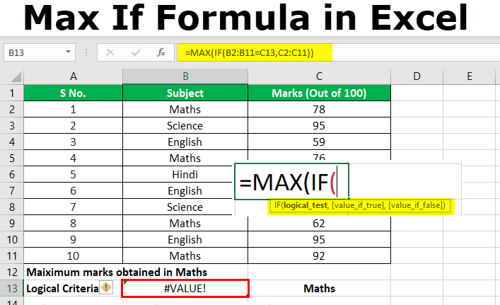
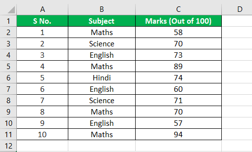
Let us consider the previous example with new numbers in column C. The following image shows the marks scored by students in various subjects. The subjects in the list are written in an unorganized manner.
Let us apply the MAX IF function to ascertain the maximum marks scored by a student in Mathematics.
We apply the following formula.
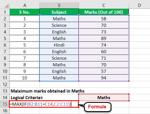
Here, the logical test is “B2:B11=C14.” The value in “B2:B11” is compared with “C14,” which is “Maths”.
The MAX IF formula returns “true” or “false” depending on the logical test. In this example, the array returns all scores of “Maths” obtained by students.
From the range “C2:C11,” the function provides values matching with “Maths.” The maximum array value matching the logical test is 94.
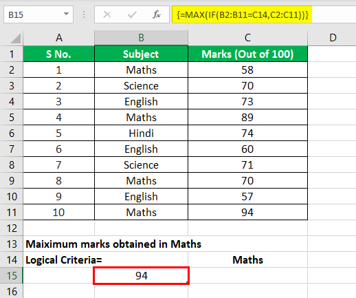
The MAX IF function is entered using “Ctrl+Shift+Enter” to get the maximum value from the given data set.
The Cautions While Using MAX IF Formula
The following points should be kept in mind while using this function:
- The variables of the logical testLogical TestA logical test in Excel results in an analytical output, either true or false. The equals to operator, “=,” is the most commonly used logical test.read more must be clearly defined; otherwise, the formula may not pass the logical test.
- The selection of cells should be in accordance with the requirement because an incorrect selection may give erroneous results.
Applications of Excel Max IF Formula
The Excel MAX IF function is used in situations where one needs to find a criteria-based maximum value from a large data set. The applications of the MAX IF function are mentioned as follows:
- It is used to find the maximum marks scored by a student in a specific subject. The data set consists of the marks obtained in multiple subjects by all students of a certain class. In such a situation, the data set is large and complex, as shown in the following image:
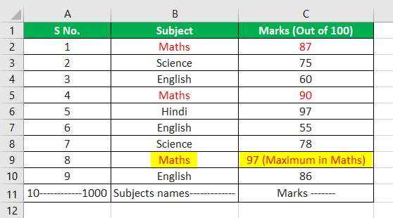
Even if the list extends to serial number 1000, the MAX IF function helps determine the maximum marks obtained by a student.
- It is used by sales professionals of MNCs to identify the city with maximum sales of specific products. An organization operating at such a large scale works with huge data sets.
- It is used by the meteorological team to find the year in which a particular month recorded the highest temperature. The temperature of different cities over several years is compared and analyzed to study variations of weather.
Frequently Asked Questions
The MAX IF function includes additional criteria with nested IF statements. The formula is stated as follows:
Alternatively, the multiplication operation can be used to handle multiple criteria. The formula is stated as follows:
The MAX IF formula can be used without an array with the help of the SUMPRODUCT function. The formula is stated as follows:
“=SUMPRODUCT(MAX((criteria_range1=criteria1)*(criteria_range2=criteria2)*max_range))”
If required, the user can add more pairs of criteria.
Note: This formula can be entered using the “Enter” key. It returns the same result as the MAX IF array formula.
The MAXIFS function determines the maximum value from a range of values. It is a criteria-based function where the criteria can be dates, numbers, text, and so on.
This function is available to users of Excel 2019 and Excel 365. The syntax of the function is stated as follows: “=MAXIFS(max_range,range1,criteria1,[range2],[criteria2],…)”
The “max_range” is the range of values from which the maximum value is to be determined. The “range1” is the first range to be evaluated. The “criteria1” is the criteria used on the first range.
Note: In the MAXIFS function, the user can enter 126 range/criteria pairs. Every range whose values are to be evaluated against a criterion must be of the same size as the “max_range.”
Key Takeaways
- The MAX function is an array formula that finds the maximum value in a given range.
- The IF function is a conditional function that displays results based on certain criteria.
- The MAX IF function identifies the maximum value from all the array values that match the logical test.
- The formula of Excel MAX If function is “=MAX(IF(logical test,value_ if _true,value_if_ false)).”
- The MAX IF formula is used to find the maximum marks obtained by a student, the maximum sales of a product, the maximum temperature of a month, and so on.
Recommended Articles
This has been a guide to MAX IF in Excel. Here we discuss how to use it to find maximum values along with practical examples and a downloadable Excel template. You may learn more about Excel from the following articles –
Источник
Author: Oscar Cronquist Article last updated on January 13, 2023

This article demonstrates how to return the latest date based on a condition using formulas or a Pivot Table. The condition is specified in cell F2 and the result is in cell F4.
For example, the condition is met in cells B5, B7, and B9. The corresponding dates in column C on the same row are 8/1/2022, 9/6/2022, and 7/29/2022.
The formula returns 9/6/2022 in cell F4 which is the last date of these dates.
Table of contents
- Lookup a value and find the most recent date
- Lookup a value and find the most recent date (Pivot Table)
- Lookup all values and find the most recent dates
- Lookup and find the most recent date using multiple conditions
- Lookup and find the most recent date on multiple sheets
- Lookup and find the most recent date, return another value on the same row
1. Lookup a value and find the most recent date
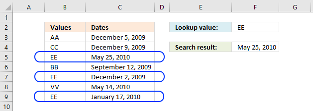
The picture above shows you values in column B (B3:B9) and dates in column C (C3:C9). The formula in cell F4 lets you search for value and return the latest date in an adjacent or corresponding column for that value.
1.0.1 Regular formula
Update, 2017-08-15! Added a regular formula.
The following formula is a regular formula, it is somewhat more complicated to understand, however, regular formulas are not prone to errors like array formulas. For example, inexperienced Excel users may easily break array formulas.
Formula in cell F4:
=MAX(INDEX((C3=A8:A14)*B8:B14,))
1.0.2 Array formula
The following formula is an array formula, section 1.2 explains how to enter an array formula.
Array formula in F4:
=MAX(IF(C3=A8:A14, B8:B14))
Section 1.3 explains how the formula above works in great detail.
How to create an array formula
1.0.3 Excel 2019 — regular formula
Formula in cell F4 (Excel 2019):
=MAXIFS(C3:C9, B3:B9,F2)
The MAXIFS function was introduced in Excel 2019, it is entered as a regular formula. You need Excel 2019 or a later Excel version to use this function.
1.0.4 Excel 365 formula
Update, 2021-09-09! Added an Excel 365 formula.
Formula in cell F4 (Excel 365):
=MAX(FILTER(C3:C9,B3:B9=F2))
The FILTER function is a new great function introduced in Excel 365.
Back to top
1.1 Watch a video where I explain the formulas
Recommended article:
Recommended articles
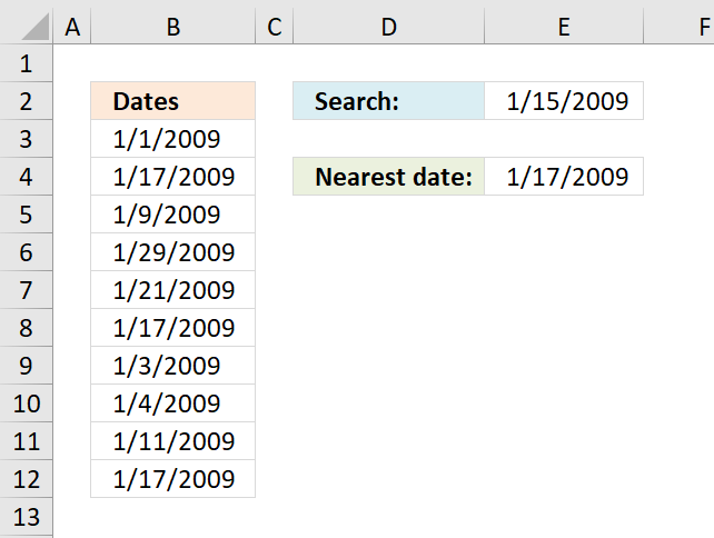
Lookup the nearest date
The image above demonstrates an array formula in cell E4 that searches for the closest date in column A to the […]
1.2 How to create an array formula
The formula in 1.0.2 is an array formula and here are the steps to enter an array formula:
- Double press with left mouse button on cell C5.
- Copy / Paste above array formula.
- Press and hold Ctrl + Shift simultaneously.
- Press Enter.
- Release all keys.
The formula changes and now begins and ends with a curly bracket, don’t enter these characters yourself. They appear automatically.
Recommended article:
Recommended articles

Back to top
1.3 Explaining array formula in cell C5
You can follow along if you select cell C5 and go to tab «Formulas» on the ribbon and then press with left mouse button on «Evaluate Formula» button. Press with left mouse button on «Evaluate» button, shown on the dialog box, to move to next step.
MAX(IF(C3=A8:A14, B8:B14))
Step 1 — Find values equal to lookup value
The equal sign is a logical operator that lets you compare value to value, in this case, a comparison value to values is performed. The output is an array of boolean values.
C3=A8:A14
becomes
«EE»={«AA»; «CC»; «EE»; «BB»; «EE»; «VV»; «EE»}
and returns
{FALSE; FALSE; TRUE; FALSE; TRUE; FALSE; TRUE}
Boolean values are either True or False, their numerical equivalents are True — 1 , False — 0 (zero).
Step 2 — Convert boolean values to corresponding dates
The IF function returns one value if the logical test is TRUE and another value if the logical test is FALSE.
IF(logical_test, [value_if_true], [value_if_false])
IF(C3=A8:A14, B8:B14)
becomes
IF({FALSE; FALSE; TRUE; FALSE; TRUE; FALSE; TRUE}, B8:B14)
becomes
IF({FALSE; FALSE; TRUE; FALSE; TRUE; FALSE; TRUE} , {40152; 40156; 40323; 40068; 40149; 40312; 40195})
and returns
{FALSE; FALSE; 40323; FALSE; 40149; FALSE; 40195}
Step 3 — Return the largest value
The MAX function allows you to calculate the largest number in a cell range. It ignores text, boolean and empty values, however, not error values.
MAX(number1, [number2], …)
MAX(IF(C3=A8:A14, B8:B14))
becomes
MAX({FALSE; FALSE; 40323; FALSE; 40149; FALSE; 40195})
and returns 40323 formatted as 2010-05-25.
1.4 Excel file
Back to top
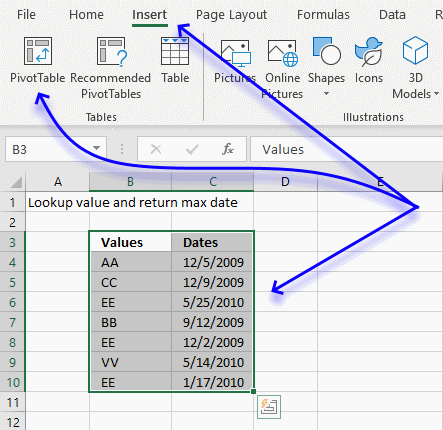
2. Lookup a value and find the most recent date (Pivot Table)
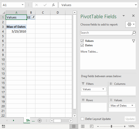
The formulas demonstrated in this article may be too slow or taking too much memory if you work with huge amounts of data. The Pivot Table is an excellent option in such cases, it is remarkably fast even with lots of data.
2.1 How to set up Pivot Table
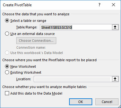
- Select the cell range containing the data.

- Go to tab «Insert» on the ribbon.
- Press with mouse on «Pivot Table» button.
- A dialog box appears.

I usually place the Pivot Table on a new worksheet so it doesn’t hide parts of the data set while filtering etc. - Press with left mouse button on OK button.
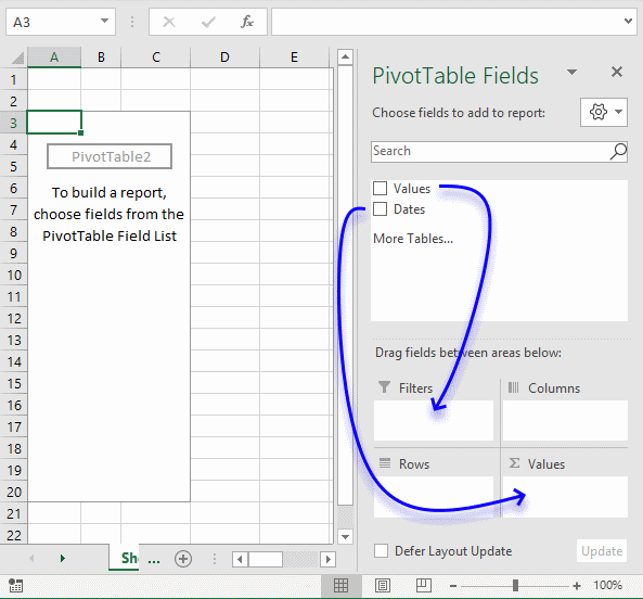
- Press with mouse on Values and drag to Filters field, see blue arrow above.
- Press with mouse on Dates and drag to Values field.
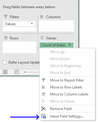
- Press with mouse on «Count of Dates».

- Press with mouse on «Value Field Settings…».

- Press with mouse on «Max» to select it.
- Press with mouse on «Number Format» button.

- Press with mouse on category «Date» and select a type.
- Press with left mouse button on OK button.
- Press with left mouse button on OK button.
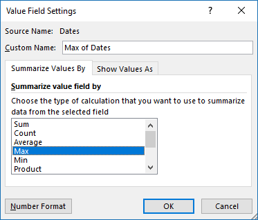
Press with mouse on cell B1 to filter the latest date based on the selected value, the image above shows value EE selected and the latest date based on that value is 5/25/2010.
Back to top
3. Lookup all values and find the most recent date
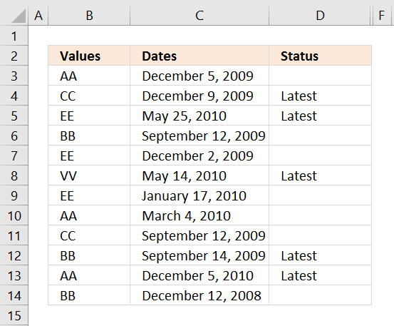
The following formula looks in column C for the most recent date based on the value in column B on the same row.
For example, cell B3 contains «AA». Cells B10 and B13 also contain «AA». The corresponding cells on the same row are C3, C10, and C13. They contain these dates «December 9, 2009», «March 4, 2010», and «December 5, 2010».
Cell D3 is not populated with the text «Latest», cell C3 is not the latest date. Cell C13 contains the last date based on the value «AA» in column B on the same row.
The following formula is a regular formula if you prefer that.
Formula in cell D3:
=IF(MAX(INDEX((B3=$B$3:$B$14)*$C$3:$C$14, ))=C3, «Latest», «»)
The next formula is an array formula, section 1.2 explains how to enter an array formula.
Array formula in cell D3:
=IF(MAX(IF(B3=$B$3:$B$14, $C$3:$C$14))=C3, «Latest», «»)
The last formula contains an Excel 2016 function, MAXIFS function.
Formula in cell D3:
=IF(MAXIFS($C$3:$C$14, $B$3:$B$14, B3)=C3, «Latest», «»)
3.1 Watch a video explaining the formula above
3.2 How to copy array formula
- Copy cell C2
- Select cell range C3:C8
- Paste
3.3 Explaining formula
This section explains the array formula.
=IF(MAX(IF(B3=$B$3:$B$14, $C$3:$C$14))=C3, «Latest», «»)
Step 1 — Identify cells that meet condition
The equal sign is a logical operator that compares value to value, it returns boolean values True or False.
B3=$B$3:$B$14
becomes
«AA»={«AA»; «CC»; «EE»; «BB»; «EE»; «VV»; «EE»; «BB»; «CC»; «VV»; «AA»; «CC»}
and returns
{TRUE; FALSE; FALSE; FALSE; FALSE; FALSE; FALSE; FALSE; FALSE; FALSE; TRUE; FALSE}.
Step 2 — Replace boolean value with corresponding dates
The IF function returns one value if the logical test is TRUE and another value if the logical test is FALSE.
IF(logical_test, [value_if_true], [value_if_false])
IF(B3=$B$3:$B$14, $C$3:$C$14)
becomes
IF({TRUE; FALSE; FALSE; FALSE; FALSE; FALSE; FALSE; FALSE; FALSE; FALSE; TRUE; FALSE}, $C$3:$C$14)
becomes
IF({TRUE; FALSE; FALSE; FALSE; FALSE; FALSE; FALSE; FALSE; FALSE; FALSE; TRUE; FALSE}, {44554; 44583; 44774; 44725; 44810; 44484; 44771; 44241; 45101; 44218; 44559; 44521})
and returns
{44554; FALSE; FALSE; FALSE; FALSE; FALSE; FALSE; FALSE; FALSE; FALSE; 44559; FALSE}
Step 3 — Extract latest date
The MAX function allows you to calculate the largest number in a cell range. It ignores text, boolean and empty values, however, not error values.
MAX(number1, [number2], …)
MAX(IF(B3=$B$3:$B$14, $C$3:$C$14))
becomes
MAX({44554; FALSE; FALSE; FALSE; FALSE; FALSE; FALSE; FALSE; FALSE; FALSE; 44559; FALSE})
and returns 44559.
Step 4 — Compare with corresponding date on the same row
MAX(IF(B3=$B$3:$B$14, $C$3:$C$14))=C3
becomes
44559=44554
and returns False.
Step 5 — Return «Latest» if True
IF(MAX(IF(B3=$B$3:$B$14, $C$3:$C$14))=C3, «Latest», «»)
becomes
IF(FALSE , «Latest», «»)
and returns «» nothing in cell D3.
3.4 Excel file
Back to top
4. Lookup and find the most recent date using multiple conditions

This example demonstrates a formula that uses two conditions to filter the latest date.
For example, the first condition is «Ram» and the second condition is «Pen». The formula calculates the latest date from column E if both conditions are true on the same row.
The first condition and the second condition are both found on rows 2 and 15, they are highlighted in the image above. The corresponding dates are 4/10/2017 and 11/1/2014, the latest date is 4/10/2017 which is returned in cell H3.
Formula in cell H3:
=MAX(INDEX((D3:D30=I2)*(E3:E30=I3)*F3:F30,))
Array formula in cell H3:
=MAX(IF((D3:D30=I2)*(E3:E30=I3),F3:F30,»»))
How to create an array formula
4.1 Explaining array formula
Step 1 — First condition
The equal sign is a logical operator that compares value to value, it returns boolean values True or False.
D3:D30=I2
becomes
{«Ram»; «Shyam»; «Ram»; «Rocky»; «John»; «Shyam»; «Rocky»; «Lalit»; «Sita»; «Rocky»; «Alex»; «Peter»; «Alex»; «Ram»; «Ram»; «Shyam»; «Ram»; «Rocky»; «John»; «Shyam»; «Rocky»; «Lalit»; «Sita»; «Rocky»; «Alex»; «Peter»; «Alex»; «Ram»}=»Ram»
and returns
{TRUE; FALSE; TRUE; FALSE; FALSE; FALSE; FALSE; FALSE; FALSE; FALSE; FALSE; FALSE; FALSE; TRUE; TRUE; FALSE; TRUE; FALSE; FALSE; FALSE; FALSE; FALSE; FALSE; FALSE; FALSE; FALSE; FALSE; TRUE}.
Step 2 — Second condition
E3:E30=I3
becomes
{«Pen»; «Pen»; 0; «Pen»; 0; 0; 0; «Pen»; «Pen»; 0; «Pen»; 0; 0; «Pen»; 0; 0; 0; «Pen»; «Pen»; 0; 0; 0; «Pen»; 0; 0; «Pen»; 0; 0}=»Pen»
and returns
{TRUE; TRUE; FALSE; TRUE; FALSE; FALSE; FALSE; TRUE; TRUE; FALSE; TRUE; FALSE; FALSE; TRUE; FALSE; FALSE; FALSE; TRUE; TRUE; FALSE; FALSE; FALSE; TRUE; FALSE; FALSE; TRUE; FALSE; FALSE}
Step 3 — Multiply arrays — AND logic
The asterisk lets you multiply arrays, this performs AND-logic meaning if both values are TRUE then return TRUE or their numerical equivalent 1. All other combinations return FALSE or 0 (zero).
The parenthesis lets you control the order of calculation, we want to compare values before we multiply the arrays.
(D3:D30=I2)*(E3:E30=I3)
becomes
({«Ram»; «Shyam»; «Ram»; «Rocky»; «John»; «Shyam»; «Rocky»; «Lalit»; «Sita»; «Rocky»; «Alex»; «Peter»; «Alex»; «Ram»; «Ram»; «Shyam»; «Ram»; «Rocky»; «John»; «Shyam»; «Rocky»; «Lalit»; «Sita»; «Rocky»; «Alex»; «Peter»; «Alex»; «Ram»}=»Ram»)*({«Pen»; «Pen»; 0; «Pen»; 0; 0; 0; «Pen»; «Pen»; 0; «Pen»; 0; 0; «Pen»; 0; 0; 0; «Pen»; «Pen»; 0; 0; 0; «Pen»; 0; 0; «Pen»; 0; 0}=»Pen»)
becomes
{TRUE; FALSE; TRUE; FALSE; FALSE; FALSE; FALSE; FALSE; FALSE; FALSE; FALSE; FALSE; FALSE; TRUE; TRUE; FALSE; TRUE; FALSE; FALSE; FALSE; FALSE; FALSE; FALSE; FALSE; FALSE; FALSE; FALSE; TRUE}*{TRUE; TRUE; FALSE; TRUE; FALSE; FALSE; FALSE; TRUE; TRUE; FALSE; TRUE; FALSE; FALSE; TRUE; FALSE; FALSE; FALSE; TRUE; TRUE; FALSE; FALSE; FALSE; TRUE; FALSE; FALSE; TRUE; FALSE; FALSE}
and returns
{1; 0; 0; 0; 0; 0; 0; 0; 0; 0; 0; 0; 0; 1; 0; 0; 0; 0; 0; 0; 0; 0; 0; 0; 0; 0; 0; 0}.
Step 4 — Replace boolean values with corresponding dates
The IF function returns one value if the logical test is TRUE and another value if the logical test is FALSE.
IF(logical_test, [value_if_true], [value_if_false])
IF((D3:D30=I2)*(E3:E30=I3),F3:F30,»»)
becomes
IF({1; 0; 0; 0; 0; 0; 0; 0; 0; 0; 0; 0; 0; 1; 0; 0; 0; 0; 0; 0; 0; 0; 0; 0; 0; 0; 0; 0}, F3:F30, «»)
becomes
IF({1; 0; 0; 0; 0; 0; 0; 0; 0; 0; 0; 0; 0; 1; 0; 0; 0; 0; 0; 0; 0; 0; 0; 0; 0; 0; 0; 0}, {42835; 41567; 41567; 41944; 41944; 42464; 42835; 41598; 41567; 42364; 42835; 41944; 42835; 41944; 42364; 42358; 41628; 41470; 42835; 42541; 41567; 41858; 42835; 41470; 41307; 42464; 42364; 42464}, «»)
and returns
{42835; «»; «»; «»; «»; «»; «»; «»; «»; «»; «»; «»; «»; 41944; «»; «»; «»; «»; «»; «»; «»; «»; «»; «»; «»; «»; «»; «»}.
Step 5 — Extract latest date
The MAX function allows you to calculate the largest number in a cell range. It ignores text, boolean and empty values, however, not error values.
MAX(number1, [number2], …)
MAX(IF((D3:D30=I2)*(E3:E30=I3),F3:F30,»»))
becomes
MAX({42835; «»; «»; «»; «»; «»; «»; «»; «»; «»; «»; «»; «»; 41944; «»; «»; «»; «»; «»; «»; «»; «»; «»; «»; «»; «»; «»; «»})
and returns 42835 (4/10/2017) which is the largest number in the array.
Back to top
4.2 Excel file
Back to top
5. Lookup and find the most recent date on multiple sheets
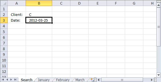
The picture above shows a workbook with 4 worksheets named «Search», January, February, and March. The formula in cell B3 looks for the latest date in all three worksheets using the condition in cell B2.
Unfortunately, it is not possible to use 3d references with IF functions. The formula contains three IF functions to make it possible to search all three worksheets.
Array formula in cell B3:
=MAX(IF(B2=January!$B$2:$B$10, January!$A$2:$A$10, «»), IF(B2=February!$B$2:$B$10, February!$A$2:$A$10, «»), IF(B2=March!$B$2:$B$10, March!$A$2:$A$10, «»))
Update! Excel 365 dynamic array formula:
=MAX(FILTER(VSTACK(January:March!A2:A10), VSTACK(January:March!B2:B10)=B2))
5.1 Explaining array formula
Step 1 — Logical test
The equal sign is a logical operator that lets you compare value to value. It is also possible to compare a value to multiple values in the same calculations, the result is an array of boolean values TRUE or FALSE.
B2=January!$B$2:$B$10
becomes
«C»={«A»; «B»; «C»; «A»; «B»; «C»; «A»; «B»; «C»}
and returns
{FALSE; FALSE; TRUE; FALSE; FALSE; TRUE; FALSE; FALSE; TRUE}.
Step 2 — Filter dates from the worksheet named January
The IF function returns one value if the logical test is TRUE and another value if the logical test is FALSE.
Function syntax: IF(logical_test, [value_if_true], [value_if_false])
IF(B2=January!$B$2:$B$10, January!$A$2:$A$10, «»)
becomes
IF({FALSE; FALSE; TRUE; FALSE; FALSE; TRUE; FALSE; FALSE; TRUE}, {40935; 40912; 40929; 40910; 40932; 40920; 40935; 40914; 40914}, «»)
and returns
{«»; «»; 40929; «»; «»; 40920; «»; «»; 40914}.
Step 3 — Logical test
B2=February!$B$2:$B$10
becomes
«C»={«A»; «B»; «C»; «A»; «B»; «C»; «A»; «B»; «C»}
and returns
{FALSE; FALSE; TRUE; FALSE; FALSE; TRUE; FALSE; FALSE; TRUE}
Step 4 — Filter dates from the worksheet named February
The IF function returns one value if the logical test is TRUE and another value if the logical test is FALSE.
Function syntax: IF(logical_test, [value_if_true], [value_if_false])
IF(B2=February!$B$2:$B$10, February!$A$2:$A$10, «»)
becomes
IF({FALSE; FALSE; TRUE; FALSE; FALSE; TRUE; FALSE; FALSE; TRUE}, {40963; 40944; 40962; 40967; 40957; 40950; 40958; 40941; 40966}, «»)
and returns
{«»; «»; 40962; «»; «»; 40950; «»; «»; 40966}.
Step 5 — Logical test
B2=March!$B$2:$B$10
becomes
«C»={«D»; «B»; «C»; «D»; «B»; «C»; «D»; «B»; «C»}
and returns
{FALSE; FALSE; TRUE; FALSE; FALSE; TRUE; FALSE; FALSE; TRUE}
Step 6 — Filter dates from worksheet named March
The IF function returns one value if the logical test is TRUE and another value if the logical test is FALSE.
Function syntax: IF(logical_test, [value_if_true], [value_if_false])
IF(B2=March!$B$2:$B$10, March!$A$2:$A$10, «»)
becomes
IF({FALSE; FALSE; TRUE; FALSE; FALSE; TRUE; FALSE; FALSE; TRUE}, {40978; 40988; 40993; 40973; 40983; 40981; 40993; 40978; 40970}, «»)
and returns
{«»; «»; 40993; «»; «»; 40981; «»; «»; 40970}.
Step 7 — Calculate largest number from three arrays
The MAX function calculate the largest number in a cell range.
Function syntax: MAX(number1, [number2], …)
MAX(IF(B2=January!$B$2:$B$10, January!$A$2:$A$10, «»), IF(B2=February!$B$2:$B$10, February!$A$2:$A$10, «»), IF(B2=March!$B$2:$B$10, March!$A$2:$A$10, «»))
becomes
MAX({«»; «»; 40929; «»; «»; 40920; «»; «»; 40914}, {«»; «»; 40962; «»; «»; 40950; «»; «»; 40966}, {«»; «»; 40993; «»; «»; 40981; «»; «»; 40970})
and returns
40993. (3/25/2012)
5.2 Lookup and find the most recent date on multiple sheets — Excel 365
Excel 365 dynamic array formula in cell B3:
=MAX(FILTER(VSTACK(January:March!A2:A10),VSTACK(January:March!B2:B10)=B2))
5.3 Explaining Excel 365 dynamic array formula
Step 1 — Create 3D reference
Here is how to create a 3D reference in cell B3:
- Select cell B3.
- Type the equal sign (=) to start creating the formula.
- Select cell range A2:A10 from the first worksheet (January).
- Press and hold CTRL key.
- Press with left mouse button on the sheet tab of the last worksheet (March) that you want to reference.
Note: To create a 3D reference, all the worksheets must be in the same workbook.
This is what the cell reference should look like in cell B3.
=January:March!A2:A10
Step 2 — Merge values from given cell ranges
The VSTACK function combines cell ranges or arrays. Joins data to the first blank cell at the bottom of a cell range or array (vertical stacking)
Function syntax: VSTACK(array1,[array2],…)
VSTACK(January:March!A2:A10)
becomes
VSTACK({40935; 40912; 40929; 40910; 40932; 40920; 40935; 40914; 40914}, {40963; 40944; 40962; 40967; 40957; 40950; 40958; 40941; 40966}, {40978; 40988; 40993; 40973; 40983; 40981; 40993; 40978; 40970})
and returns
{40935; 40912; 40929; 40910; 40932; 40920; 40935; 40914; 40914; 40963; 40944; 40962; 40967; 40957; 40950; 40958; 40941; 40966; 40978; 40988; 40993; 40973; 40983; 40981; 40993; 40978; 40970}
Step 3 — Create a logical array containing TRUE or FALSE based on the condition specified in cell B2
This part of the formula merges the values in cell ranges B2:B10 in worksheets from January to March.
The equal sign compares the values to the specified condition in cell B2, the result is a boolean array containing TRUE or FALSE.
VSTACK(January:March!B2:B10)=B2
becomes
{«A»; «B»; «C»; «A»; «B»; «C»; «A»; «B»; «C»; «A»; «B»; «C»; «A»; «B»; «C»; «A»; «B»; «C»; «D»; «B»; «C»; «D»; «B»; «C»; «D»; «B»; «C»}=»C»
and returns
{FALSE; FALSE; TRUE; FALSE; FALSE; TRUE; FALSE; FALSE; TRUE; FALSE; FALSE; TRUE; FALSE; FALSE; TRUE; FALSE; FALSE; TRUE; FALSE; FALSE; TRUE; FALSE; FALSE; TRUE; FALSE; FALSE; TRUE}.
The semicolon ; is a row delimiting character in Excel arrays.
Step 3 — Filter dates based on the condition specified in cell B2
The FILTER function extracts values/rows based on a condition or criteria.
Function syntax: FILTER(array, include, [if_empty])
FILTER(VSTACK(January:March!A2:A10),VSTACK(January:March!B2:B10)=B2)
becomes
FILTER({40935; 40912; 40929; 40910; 40932; 40920; 40935; 40914; 40914; 40963; 40944; 40962; 40967; 40957; 40950; 40958; 40941; 40966; 40978; 40988; 40993; 40973; 40983; 40981; 40993; 40978; 40970}, {FALSE; FALSE; TRUE; FALSE; FALSE; TRUE; FALSE; FALSE; TRUE; FALSE; FALSE; TRUE; FALSE; FALSE; TRUE; FALSE; FALSE; TRUE; FALSE; FALSE; TRUE; FALSE; FALSE; TRUE; FALSE; FALSE; TRUE})
and returns
{40929; 40920; 40914; 40962; 40950; 40966; 40993; 40981; 40970}.
Step 4 — Get the latest date
The MAX function calculate the largest number in a cell range.
Function syntax: MAX(number1, [number2], …)
MAX(FILTER(VSTACK(January:March!A2:A10),VSTACK(January:March!B2:B10)=B2))
becomes
MAX({40929; 40920; 40914; 40962; 40950; 40966; 40993; 40981; 40970})
and returns
40993. 40993 represents the date 3/25/2012 in Excel.
5.4 Get Excel file
Back to top
6. Lookup and find the most recent date, return the corresponding value on the same row
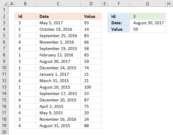
Enter a condition in cell G3, the formula extracts the latest date. Another formula in cell G3 gets the corresponding value on the same row from column D.
Array formula in cell G3:
=MAX((B3:B19=G2)*C3:C19)
If you prefer a regular formula in G3:
=MAX(INDEX((B3:B19=G2)*C3:C19,))
Update! New array formula in cell G4:
=INDEX(D3:D19,MATCH(1,(B3:B19=G2)*(C3:C19=G3),0))
Excel 365 formula in cell G4:
=FILTER(D3:D19,(B3:B19=G2)*(G3=C3:C19))
Old Formula in cell G4:
=INDEX($D$3:$D$19, SUMPRODUCT((B3:B19=G2)*(G3=C3:C19)*MATCH(ROW(B3:B19), ROW(B3:B19))))
6.1 Watch a video explaining the formulas above
6.2 Explaining formula in cell G4
Formulas in cell G3 are explained in section 1 above.
Step 1 — First condition
The equal sign is a logical operator that lets you compare value to value or in this case value to an array of values. The result is an array of boolean values TRUE and FALSE.
This logical expression compares the condition specified in cell G2 to the values in B3:B19.
B3:B19=G2
becomes
{3; 1; 2; 4; 4; 1; 3; 1; 3; 4; 1; 3; 4; 3; 4; 3; 4}=3
and returns
{TRUE; FALSE; FALSE; FALSE; FALSE; FALSE; TRUE; FALSE; TRUE; FALSE; FALSE; TRUE; FALSE; TRUE; FALSE; TRUE; FALSE}.
Step 2 — Second condition
C3:C19=G3
becomes
{42860; 42662; 42638; 42675; 42266; 42413; 42977; 42362; 42736; 42094; 42236; 42264; 42358; 42096; 42133; 42690; 42247}=42977
and returns
{FALSE; FALSE; FALSE; FALSE; FALSE; FALSE; TRUE; FALSE; FALSE; FALSE; FALSE; FALSE; FALSE; FALSE; FALSE; FALSE; FALSE}
Step 3 — Multiply arrays to perform AND logic
The asterisk character lets you multiply numbers in an Excel formula. The parentheses lets you control the order of operation.
(B3:B19=G2)*(C3:C19=G3)
becomes
({TRUE; FALSE; FALSE; FALSE; FALSE; FALSE; TRUE; FALSE; TRUE; FALSE; FALSE; TRUE; FALSE; TRUE; FALSE; TRUE; FALSE})*({FALSE; FALSE; FALSE; FALSE; FALSE; FALSE; TRUE; FALSE; FALSE; FALSE; FALSE; FALSE; FALSE; FALSE; FALSE; FALSE; FALSE})
and returns
{0; 0; 0; 0; 0; 0; 1; 0; 0; 0; 0; 0; 0; 0; 0; 0; 0}
Step 4 — Find the relative position
The MATCH function returns the relative position of an item in an array that matches a specified value in a specific order.
Function syntax: MATCH(lookup_value, lookup_array, [match_type])
MATCH(1,(B3:B19=G2)*(C3:C19=G3),0)
becomes
MATCH(1,{0; 0; 0; 0; 0; 0; 1; 0; 0; 0; 0; 0; 0; 0; 0; 0; 0},0)
and returns 7.
Number 1 is in position 7 in the array.
Step 5 — Get value based on the relative position
The INDEX function returns a value or reference from a cell range or array, you specify which value based on a row and column number.
Function syntax: INDEX(array, [row_num], [column_num])
INDEX(D3:D19,MATCH(1,(B3:B19=G2)*(C3:C19=G3),0))
becomes
INDEX(D3:D19,7)
and returns the value in cell D9 which is 59.
Back to top
Return to Excel Formulas List
Download Example Workbook
Download the example workbook
This tutorial will demonstrate how to calculate the max date in Excel and Google Sheets. It will also demonstrate how to lookup the max date in a list and return a corresponding value.
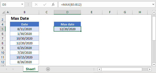
Calculate Max Date
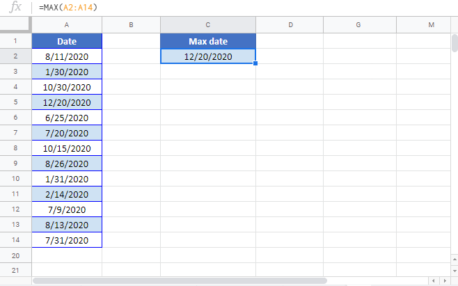
You can use the MAX Function to calculate the max date in a list:
=MAX(B3:B15)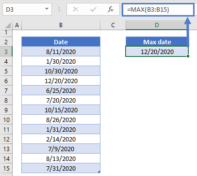
Max Date Lookup
After calculating the max date, you can perform a VLOOKUP (or XLOOKUP) to return a value corresponding to that date:
=VLOOKUP(E3,B3:C15,2,FALSE)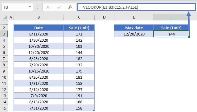
Max Date Sum
Alternatively, you can use the SUMIF Function to total all the values associated with that date from a list:
=SUMIF(B3:B15,E3,C3:C15)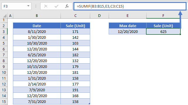
Google Sheets – Max Date
All of the above examples work exactly the same in Google Sheets as in Excel.
Column A is date
Column B is criteria
I want to find the MIN date for each criteria. I tried using Ctrl+Shift+Enter with
=MIN(MATCH(B2,B:B,0))
but thats not quite right because I need to refer to Column A somehow to get the date. I’m pretty confident this can be done with arrays, so any help would be great.
![]()
Ram
3,08410 gold badges40 silver badges56 bronze badges
asked May 24, 2012 at 23:46
![]()
1
Try this (array formula):
=MIN(IF(B2=B:B,A:A))
answered May 25, 2012 at 1:47
![]()
andy holadayandy holaday
2,2821 gold badge16 silver badges25 bronze badges
6
An even more compact array formula is:
=MINIF(B2=B:B,A:A)
NOTE 1: Complete using Ctrl+Shift+Enter to enter the formula as an array formula.
NOTE 2: The two-formula method (i.e., using =MIN(IF(B2=B:B,A:A))) is more flexible and works in more cases than the single-formula method shown here but I’ve included it as an answer as a possible option.
answered Aug 15, 2018 at 10:40
![]()
=SMALL(INDEX(($F$2:$F$14=F3)*$D$2:$D$14,),SUM(COUNTA(F:F)-COUNTIF(F:F,F3)))
If your criteria is repeated and want to find the min date for that you can use this without shift+ctrl + enter function.
- date is
Dcolumn - criteria is
Fcolumn
![]()
Samuel Hulla
6,3477 gold badges34 silver badges66 bronze badges
answered Sep 28, 2018 at 7:15
![]()