
Excel MAX IF Function (Table of Contents)
- MAX IF in Excel
- How to Use MAX IF Function in Excel?
MAX IF in Excel
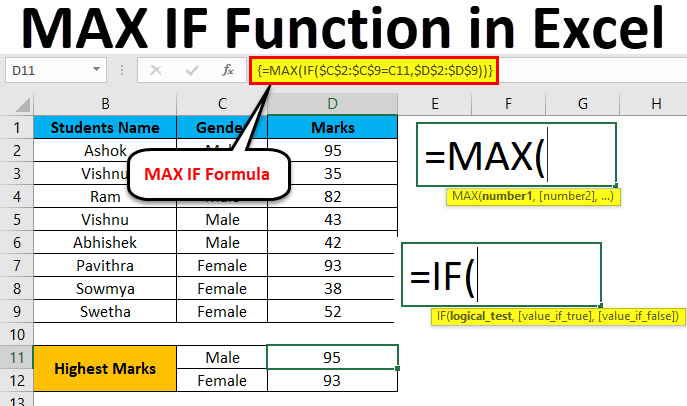
Max function and IF function in Excel are used to find the maximum value from the given range of datasets with the defined criteria. The MAX function returns the maximum value from the select number range, and the IF function helps find that number with chosen criteria. For this, we can first apply the IF function where, as per syntax, first choose Criteria Range and with the criteria we want, then select the value range. Once done, then cover the complete IF function in the MAX function’s syntax with curly brackets.
In Microsoft Excel, there is no such separate syntax for the MAXIF function, but we can combine the MAX and IF function in an array formula.
MAX Formula in Excel
Below is the MAX Formula in Excel:
Arguments of MAX Formula:
- number1: This number1 refers to a numeric value or range which contains a numeric value.
- number2 [optional]: This number2 refers to a numeric value or range which contains a numeric value.
IF Formula in Excel
Below is the IF Formula in Excel:
Arguments of IF Formula:
- Logical test: Which is a logical expression value to check the value is TRUE or FALSE.
- value _if_ true: Which is a value that returns if the logical test is true.
- value _if_ false: Which is a value that returns if the logical test is false.
How to Use MAX IF Function in Excel?
MAX and IF Functions in Excel is very simple and easy to use. Let’s understand the working of the MAX IF Function in Excel with some example.
You can download this MAX IF Function Excel Template here – MAX IF Function Excel Template
Example #1 – MAX Function in Excel
In this example, we will first learn how to use the MAX function with the below example.
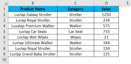
Consider the below example, which shows sales data of the product category wise.
Now we will use the MAX function to find out which has the largest sales value by following the below steps.
Step 1 – First, select the new cell, i.e. D11.
Step 2 – Apply the MAX function i.e. =MAX(D2:D9)
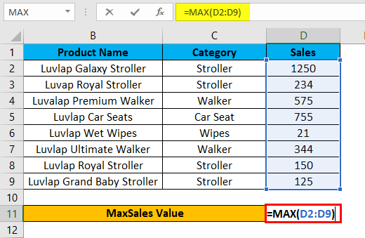
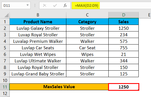
Step 3 – Press enter so that we will get the MAX value is 1250, which is shown in the below screenshot.
In the below result, the Max function will check for the largest number in the D column and return the maximum sales value as 1250.
Example #2 – Using MAX IF Function in Excel with an array formula
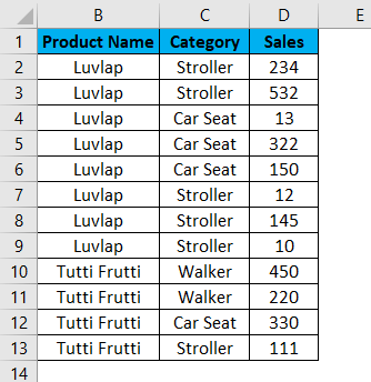
In this example, we will learn how to use MAX IF function in Excel. Assume that we need to check the largest sales value category wise. Using only the max function, we can check only the maximum value, but we cannot check the maximum value category wise if the sales data contain a huge category and sales value.
In such a case, we can combine MAX and If Function with an array formula so that it makes the task very easier to find out the largest sales value category wise in Excel.
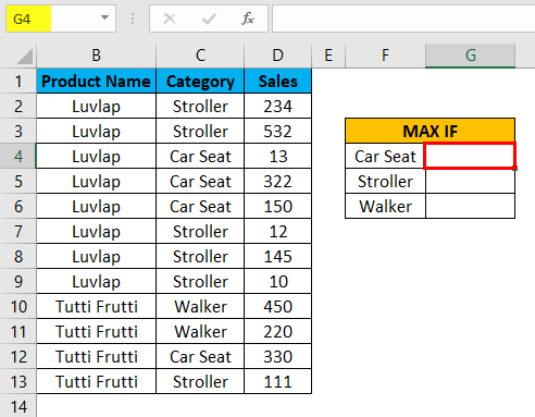
Consider the below example, which has Product Name, Category and Sales value which is shown below.
Now we will apply the Excel MAX IF function to find out the maximum sales value by following the below steps.
Step 1 – First, we will create a new table with a category name to display the result, as shown below.
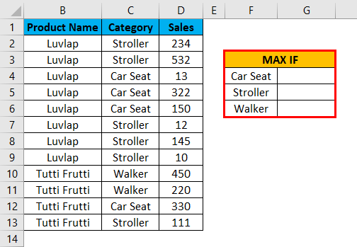
Step 2 – Select cell G4.
Step 3 – Apply the MAX IF formula i.e. =MAX(IF(C$2:C13=F4,D2:D13))
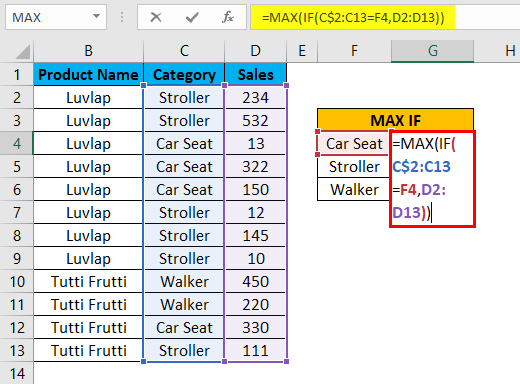
In the above formula, we have applied MAX and IF function and then we selected Column C2 to C13 where we have listed the category name as C2:C13 and then we have checked the condition by selecting the cell as F4 where the F4 column is nothing but Category Name.
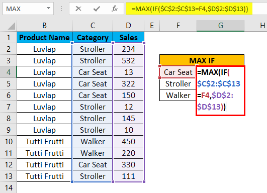
Now the if condition will check for the entire category name in C2 to C13 column whether it matches with the mentioned Category name in the F4 column; if the category name matches, it will return the largest sales value from the selected D column as D2 to D13 and lock the cells by pressing F4 where we will get the $ symbol to indicate that cells are locked, and we have given the Formula as =MAX(IF($C$2:$C$13=F4,$D$2:$D$13)).
After the MAXIF function is completed by closing all the brackets now, hold SHIFT+CTRL and then press enter as SHIFT+CTRL+ENTER so that we will get the output in array formula where we will get open and closing parenthesis at the opening and end of the statement, which is shown in the below screenshot.
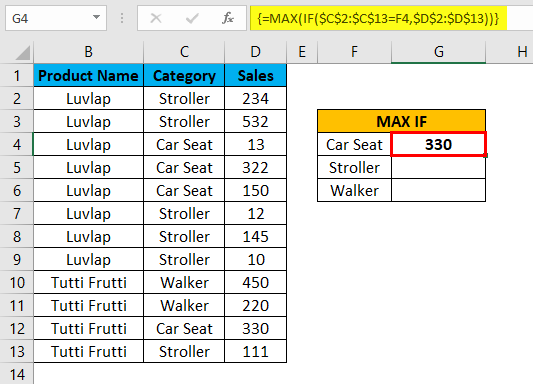
Here as we can see in the above screenshot MAX IF function check for the category name in the D column as well as in the F column, and if it matches, it will return the largest value; here in this example, we got the output as 330 which is a largest sales value in the category.
Now drag down the MAX IF formulas for all the cell so that we will get the output result which is shown below.
Example #3 – Using MAX IF Function in Excel with an array formula
In this example, we will use the same Excel MAX IF function to find out the highest marks from a set of students.
Consider the below example, which shows student name along with their Gender and Marks, which is shown below.
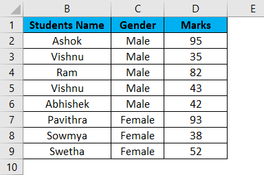
Here in this example, we are going to find out Gender wise who has scored the highest marks by following the below steps.
Step 1 – First, create a new table with Male and Female as a separate column to display the result, which is shown below.
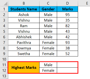
Step 2 – Now, we will apply the Excel MAX IF function as follows. Select cell D11.
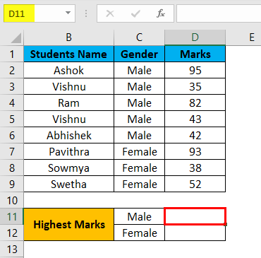
Step 3 – Insert the MAX IF function by selecting the Gender column from C2 to C9.
Now we have to give the condition as IF(C2:C9=C11,D2:D9), which means that the IF condition will check for the gender from the C2 column whether it matches with C11 and If the gender matches MAX IF function returns the highest value.
Step 4 – Now lock the cells by pressing F4 so that the selected cells will be locked, which is shown in the below screenshot.
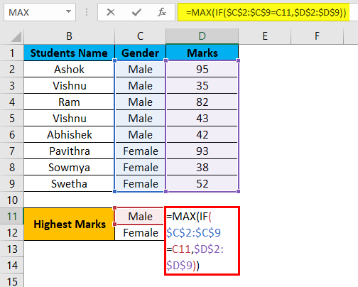
Step 5 – Once we complete the MAXIF function, Hit SHIFT+CRL+ENTER to make it an array formula to see the opening and closing parenthesis in the MAX IF function, which is shown below.
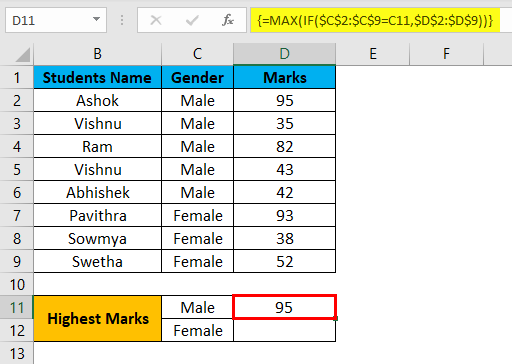
We can see that we got the highest mark as 95 for the gender MALE in the above screenshot.
Step 6 – Drag down the formula for all the below cells so that we will get the output as shown below.
In the above result using the Excel MAX IF function, we have found the highest marks gender-wise where MALE has scored 95 as the highest mark, and for FEMALE, we got 93 as the Highest mark.
Things to Remember
- In Microsoft Excel, there is no such MAX IF function as SUMIF and COUNTIF.
- We can use the MAX and IF function by combining them in the formulation.
- MAX IF function will throw an error #VALUE! If we did not apply the SHIFT+ENTER +KEY, make sure that you are using MAX IF function as an array formula.
Recommended Articles
This has been a guide to MAX IF in Excel. Here we discuss how to use MAX IF Function in Excel along with practical examples and downloadable excel templates. You can also go through our other suggested articles –
- MAX Excel Function
- SUMIF in Excel
- Excel SUM MAX MIN AVERAGE
- MAX Formula in Excel
What is MAX IF Formula in Excel?
The MAX IF formula is a combination of two excel functions (MAX and IF Function) that identifies the maximum value from all the outcome that matches the logical test. MAX IF is used as an array formula where the logical test can run multiple times in a data set.
The method to use MAX IF function together is as follows:
=MAX(IF(logical test,value_ if _true,value_ if_ false))
Being an array formula, it should always be used by pressing “Ctrl+Shift+Enter” while running the formula.
Table of contents
- What is MAX IF Formula in Excel?
- How to use Max If Formula in Excel?
- The Cautions While Using MAX IF Formula
- Applications of Excel Max IF Formula
- Frequently Asked Questions
- Recommended Articles
You are free to use this image on your website, templates, etc, Please provide us with an attribution linkArticle Link to be Hyperlinked
For eg:
Source: Max IF in Excel (wallstreetmojo.com)
How to use Max If Formula in Excel?
You can download this Max If Formula Excel Template here – Max If Formula Excel Template
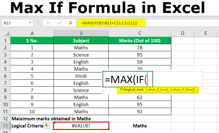
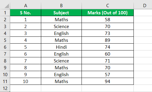
Let us consider the previous example with new numbers in column C. The following image shows the marks scored by students in various subjects. The subjects in the list are written in an unorganized manner.
Let us apply the MAX IF function to ascertain the maximum marks scored by a student in Mathematics.
We apply the following formula.
“=MAX(IF(B2:B11=C14,C2:C11))”
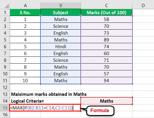
Here, the logical test is “B2:B11=C14.” The value in “B2:B11” is compared with “C14,” which is “Maths”.
The MAX IF formula returns “true” or “false” depending on the logical test. In this example, the array returns all scores of “Maths” obtained by students.
From the range “C2:C11,” the function provides values matching with “Maths.” The maximum array value matching the logical test is 94.
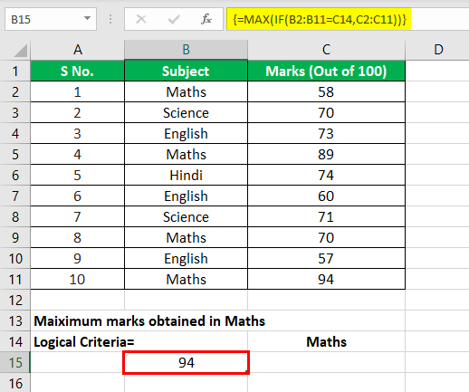
The MAX IF function is entered using “Ctrl+Shift+Enter” to get the maximum value from the given data set.
The Cautions While Using MAX IF Formula
The following points should be kept in mind while using this function:
- The variables of the logical testA logical test in Excel results in an analytical output, either true or false. The equals to operator, “=,” is the most commonly used logical test.read more must be clearly defined; otherwise, the formula may not pass the logical test.
- The selection of cells should be in accordance with the requirement because an incorrect selection may give erroneous results.
Applications of Excel Max IF Formula
The Excel MAX IF function is used in situations where one needs to find a criteria-based maximum value from a large data set. The applications of the MAX IF function are mentioned as follows:
- It is used to find the maximum marks scored by a student in a specific subject. The data set consists of the marks obtained in multiple subjects by all students of a certain class. In such a situation, the data set is large and complex, as shown in the following image:
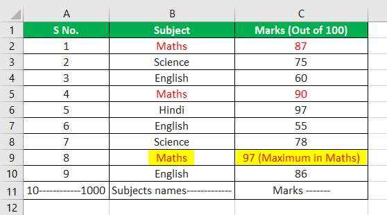
Even if the list extends to serial number 1000, the MAX IF function helps determine the maximum marks obtained by a student.
- It is used by sales professionals of MNCs to identify the city with maximum sales of specific products. An organization operating at such a large scale works with huge data sets.
- It is used by the meteorological team to find the year in which a particular month recorded the highest temperature. The temperature of different cities over several years is compared and analyzed to study variations of weather.
Frequently Asked Questions
#1 – How to use MAX IF formula with multiple criteria?
The MAX IF function includes additional criteria with nested IF statements. The formula is stated as follows:
“{=MAX(IF(criteria_range1=criteria1,IF(criteria_range2=criteria2,max_range)))}”
Alternatively, the multiplication operation can be used to handle multiple criteria. The formula is stated as follows:
“{=MAX(IF((criteria_range1=criteria1)*(criteria_range2=criteria2), max_range))}”
#2 – How to use MAX IF formula without an array?
The MAX IF formula can be used without an array with the help of the SUMPRODUCT function. The formula is stated as follows:
“=SUMPRODUCT(MAX((criteria_range1=criteria1)*(criteria_range2=criteria2)*max_range))”
If required, the user can add more pairs of criteria.
Note: This formula can be entered using the “Enter” key. It returns the same result as the MAX IF array formula.
#3 – What is the MAXIFS function of Excel?
The MAXIFS function determines the maximum value from a range of values. It is a criteria-based function where the criteria can be dates, numbers, text, and so on.
This function is available to users of Excel 2019 and Excel 365. The syntax of the function is stated as follows: “=MAXIFS(max_range,range1,criteria1,[range2],[criteria2],…)”
The “max_range” is the range of values from which the maximum value is to be determined. The “range1” is the first range to be evaluated. The “criteria1” is the criteria used on the first range.
Note: In the MAXIFS function, the user can enter 126 range/criteria pairs. Every range whose values are to be evaluated against a criterion must be of the same size as the “max_range.”
- The MAX function is an array formula that finds the maximum value in a given range.
- The IF function is a conditional function that displays results based on certain criteria.
- The MAX IF function identifies the maximum value from all the array values that match the logical test.
- The formula of Excel MAX If function is “=MAX(IF(logical test,value_ if _true,value_if_ false)).”
- The MAX IF formula is used to find the maximum marks obtained by a student, the maximum sales of a product, the maximum temperature of a month, and so on.
Recommended Articles
This has been a guide to MAX IF in Excel. Here we discuss how to use it to find maximum values along with practical examples and a downloadable Excel template. You may learn more about Excel from the following articles –
- Examples of IF Formula in Excel
- How to Add Borders in Excel?
- VLOOKUP Function in VBA Excel
- SUMPRODUCT Function with Multiple Criteria
Содержание
- Max IF in Excel
- What is MAX IF Formula in Excel?
- How to use Max If Formula in Excel?
- The Cautions While Using MAX IF Formula
- Applications of Excel Max IF Formula
- Frequently Asked Questions
- Key Takeaways
- Recommended Articles
- Max if criteria match
- Related functions
- Summary
- Generic formula
- Explanation
- With MAXIFS
- Maximum if multiple criteria
- Related functions
- Summary
- Generic formula
- Explanation
- Excel Table
- MAXIFS function
- Maximum value if
- Related functions
- Summary
- Generic formula
- Explanation
- Excel Table
- MAXIFS function
- MAX + FILTER
- Summary table with BYROW
- MAX + IF
Max IF in Excel


What is MAX IF Formula in Excel?
The MAX IF formula is a combination of two excel functions (MAX and IF Function) that identifies the maximum value from all the outcome that matches the logical test. MAX IF is used as an array formula where the logical test can run multiple times in a data set.
The method to use MAX IF function together is as follows:
=MAX(IF(logical test,value_ if _true,value_ if_ false))
Being an array formula, it should always be used by pressing “Ctrl+Shift+Enter” while running the formula.
Table of contents
You are free to use this image on your website, templates, etc., Please provide us with an attribution link How to Provide Attribution? Article Link to be Hyperlinked
For eg:
Source: Max IF in Excel (wallstreetmojo.com)
How to use Max If Formula in Excel?
Let us consider the previous example with new numbers in column C. The following image shows the marks scored by students in various subjects. The subjects in the list are written in an unorganized manner.
Let us apply the MAX IF function to ascertain the maximum marks scored by a student in Mathematics.
We apply the following formula.
Here, the logical test is “B2:B11=C14.” The value in “B2:B11” is compared with “C14,” which is “Maths”.
The MAX IF formula returns “true” or “false” depending on the logical test. In this example, the array returns all scores of “Maths” obtained by students.
From the range “C2:C11,” the function provides values matching with “Maths.” The maximum array value matching the logical test is 94.
The MAX IF function is entered using “Ctrl+Shift+Enter” to get the maximum value from the given data set.
The Cautions While Using MAX IF Formula
The following points should be kept in mind while using this function:
- The variables of the logical testLogical TestA logical test in Excel results in an analytical output, either true or false. The equals to operator, “=,” is the most commonly used logical test.read more must be clearly defined; otherwise, the formula may not pass the logical test.
- The selection of cells should be in accordance with the requirement because an incorrect selection may give erroneous results.
Applications of Excel Max IF Formula
The Excel MAX IF function is used in situations where one needs to find a criteria-based maximum value from a large data set. The applications of the MAX IF function are mentioned as follows:
- It is used to find the maximum marks scored by a student in a specific subject. The data set consists of the marks obtained in multiple subjects by all students of a certain class. In such a situation, the data set is large and complex, as shown in the following image:
Even if the list extends to serial number 1000, the MAX IF function helps determine the maximum marks obtained by a student.
- It is used by sales professionals of MNCs to identify the city with maximum sales of specific products. An organization operating at such a large scale works with huge data sets.
- It is used by the meteorological team to find the year in which a particular month recorded the highest temperature. The temperature of different cities over several years is compared and analyzed to study variations of weather.
Frequently Asked Questions
The MAX IF function includes additional criteria with nested IF statements. The formula is stated as follows:
Alternatively, the multiplication operation can be used to handle multiple criteria. The formula is stated as follows:
The MAX IF formula can be used without an array with the help of the SUMPRODUCT function. The formula is stated as follows:
“=SUMPRODUCT(MAX((criteria_range1=criteria1)*(criteria_range2=criteria2)*max_range))”
If required, the user can add more pairs of criteria.
Note: This formula can be entered using the “Enter” key. It returns the same result as the MAX IF array formula.
The MAXIFS function determines the maximum value from a range of values. It is a criteria-based function where the criteria can be dates, numbers, text, and so on.
This function is available to users of Excel 2019 and Excel 365. The syntax of the function is stated as follows: “=MAXIFS(max_range,range1,criteria1,[range2],[criteria2],…)”
The “max_range” is the range of values from which the maximum value is to be determined. The “range1” is the first range to be evaluated. The “criteria1” is the criteria used on the first range.
Note: In the MAXIFS function, the user can enter 126 range/criteria pairs. Every range whose values are to be evaluated against a criterion must be of the same size as the “max_range.”
Key Takeaways
- The MAX function is an array formula that finds the maximum value in a given range.
- The IF function is a conditional function that displays results based on certain criteria.
- The MAX IF function identifies the maximum value from all the array values that match the logical test.
- The formula of Excel MAX If function is “=MAX(IF(logical test,value_ if _true,value_if_ false)).”
- The MAX IF formula is used to find the maximum marks obtained by a student, the maximum sales of a product, the maximum temperature of a month, and so on.
Recommended Articles
This has been a guide to MAX IF in Excel. Here we discuss how to use it to find maximum values along with practical examples and a downloadable Excel template. You may learn more about Excel from the following articles –
Источник
Max if criteria match

Summary
To find the maximum value in a range with specific criteria, you can use a basic array formula based on the IF function and MAX function. In the example shown, the formula in cell H8 is:
which returns the maximum temperature on the date in H7.
Note: this is an array formula and must be entered with Control + Shift + Enter
Generic formula
Explanation
The example shown contains almost 10,000 rows of data. The data represents temperature readings taken every 2 minutes over a period of days. For any given date (provided in cell H7), we want to get the maximum temperature on that date.
Inside the IF function, logical test is entered as B5:B9391=H7. Because we’re comparing the value in H7 against a range of cells (an array), the result will be an array of results, where each item in the array is either TRUE or FALSE. The TRUE values represent dates that match H7.
For the value if true, we provide the range E5:E9391, which fetches all the full set of temperatures in Fahrenheit. This returns an array of values the same size as the first array.
The IF function acts as a filter. Because we provide IF with an array for the logical test, IF returns an array of results. Where the date matches H7, the array contains a temperature value. In all other cases, the array contains FALSE. In other words, only temperatures associated with the date in H7 survive the trip through the IF function.
The array result from the IF function is delivered directly to the MAX function, which returns the maximum value in the array.
With MAXIFS
In Excel O365 and Excel 2019, the new MAXIFS function can find the maximum value with one or more criteria without the need for an array formula. With MAXIFS, the equivalent formula for the this example is:
Источник
Maximum if multiple criteria
Summary
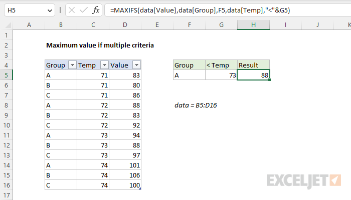
To get the maximum value in a set of data that meets multiple criteria, you can use a formula based on the MAXIFS function. In the example shown, the formula in H5 is:
With «A» in cell F5 and the number 73 in cell G5, the result is 88. This is the maximum value in group «A» below a temperature of 73.
Generic formula
Explanation
In this example, the goal is to get the maximum value for a given group below a specific temperature. In other words, we want the max value after applying multiple criteria. The easiest way to solve this problem is with the MAXIFS function. However, if you need more flexibility (i.e. you need to work with arrays and not ranges), you can use the MAX function with the FILTER function. In older versions of Excel without MAXIFS or FILTER, you can use a traditional array formula based on the MAX function and the IF function. Each approach is explained below.
Excel Table
For convenience, all data is in an Excel Table named data in the range B5:D16. Excel Tables are a convenient way to work with data in Excel because they (1) automatically expand to include new data and (2) offer structured references, which allow you to refer to data by name instead of by address. If you are new to Excel Tables, this article provides an overview.
MAXIFS function
One way to solve this problem is with the MAXIFS function, which can get the maximum value in a range based on one or more criteria. The generic syntax for MAXIFS with two conditions looks like this:
Note that each condition is defined by two arguments: range1 and criteria1 define the first condition, and range2 and criteria2 define the second condition. All conditions must be true in order for value to be considered. We start off with the max_range, which is the Value column in the table:
Next, we add criteria to test for the group value entered in cell F5:
If we enter the formula above as-is, we will get the maximum value in group «A». Next, we need to add a second condition to further restrict values below the temperature entered in cell G5:
Notice we need to concatenate the less than operator («
Источник
Maximum value if
Summary
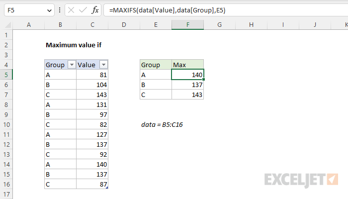
To get the max value if a condition is true, you can use the MAXIFS function. In the example shown, the formula in cell F5 is:
Where data is an Excel Table in the range B5:C16. As the formula is copied down, the result is the maximum value for each group listed in column E. There are several ways to approach this problem. See below for other formula options, including an all-in-one formula that creates a dynamic summary table.
Generic formula
Explanation
In this example, the goal is to get the maximum value for each group in the data as shown. The easiest way to solve this problem is with the MAXIFS function. However, there are actually several options. If you need more flexibility (i.e. you need to work with arrays and not ranges), you can use the MAX function with the FILTER function. To create a dynamic summary table with a single all-in-one formula, you can use the BYROW function. In older versions of Excel without the MAXIFS function, you can use an array formula based on the MAX function and the IF function. Each approach is explained below.
Excel Table
For convenience, all data is in an Excel Table named data in the range B5:C16. Excel Tables are a convenient way to work with data in Excel because they (1) automatically expand to include new data and (2) offer structured references, which allow you to refer to columns by name instead of by address. If you are new to Excel Tables, this article provides an overview.
MAXIFS function
The MAXIFS function can get the maximum value in a range based on one or more criteria. The generic syntax for MAXIFS with a single condition looks like this:
Note that the condition is defined with two arguments: range1 and criteria1. In this problem, the condition is that the group value in column B must equal the group value in column E. We start off with the max_range, which is the Value column:
Next, we add the criteria range, which is the Group column:
Finally, we add the criteria itself, the value in cell E5:
As the formula is copied down, the table references behave like absolute references and don’t change. The reference to E5 is relative and changes at each new row. The result is the maximum value for each group listed in column E.
The MAXIFS function is a straightforward solution that works well. However, it does have one significant limitation: the range arguments inside MAXIFS must be actual ranges, you can’t substitute arrays. If you need to use arrays, see the MAX + FILTER option, or the all-in-one summary table formula based on the BYROW function below.
MAX + FILTER
In the dynamic array version of Excel, another way to solve this problem is with the MAX function and the FILTER function like this:
Inside the MAX function, the FILTER function is configured to filter values by group:
Array is provided as the Value column in the table, and the include argument is a simple expression:
With «A» in cell E5, the expression above returns an array like this:
Because there are 12 values in Group, there are 12 TRUE and FALSE results. The TRUE values correspond to values in the table associated with group A. With the array above acting as a filter, the FILTER function returns an array that contains the four values in group A directly to the MAX function:
MAX then returns a final result of 140. The primary advantage of using the MAX function with the FILTER function is that you are not required to supply a range of values on the worksheet. You can instead provide an array of values created with another operation. This is very useful when the source data needs to be manipulated in some way before a max value is calculated.
Summary table with BYROW
In the latest version of Excel, which supports dynamic array formulas, you can create a single all-in-one formula that builds the entire summary table, including headers, like this:
The LET function is used to assign four intermediate variables: groups, values, ugroups, and results. Both groups and values are simple assignments to rows in the table:
This is done primarily to make the formula more portable. Defining these variables here keeps all of the worksheet references at the top of the formula where they can be easily changed.
In our summary table, we want a list of unique groups, so we define ugroups (unique groups) with the UNIQUE function like this:
From the 12 rows in the data, the UNIQUE function returns just 3 unique groups:
Note: you could run groups through the SORT function to ensure that groups are in the correct order. In this case the source data already shows groups in order, so it is not necessary.
At this point, we are ready to calculate the max values for in each group. We do this with the BYROW function which calculates the maximum values and assigns the result to the variable results:
BYROW runs through the ugroups values row by row. At each row, it applies this calculation:
The value r is the unique group in the «current» row in the summary table. Inside the MAX function, the FILTER function is configured to filter values by group like this:
In the first row (group A), the result from FILTER is an array like this:
This array is delivered directly to the MAX function, which returns the maximum number. When BYROW is finished, we have an array with 3 numbers (one for each group) like this:
This array is the value assigned to results. Finally the HSTACK and VSTACK functions are used to assemble a complete table:
At the top of the table, the array constant <«Group»,»Max»>creates a header row. The HSTACK function combines ugroups and results horizontally, and VSTACK combines the header row and the data to make the final table. The final result spills into multiple cells on the worksheet.
MAX + IF
In older versions of Excel that do not have the MAXIFS function, you can solve this problem with an array formula based on the MAX function and the IF function like this:
Note: this is an array formula and must be entered with control + shift + enter in Legacy Excel.
Working from the inside out, the IF function is evaluated first. The logical test is an expression that tests the entire Group column against the value in cell E5:
Because there are 12 values in data[Group], the result is an array with 12 TRUE / FALSE values like this:
The TRUE values correspond to rows where the group is «A». For all other groups, the value is FALSE. For value_if_true, we supply the Value column, and we omit value_if_false altogether:
The final result from IF is an array like this:
Looking at the values in this array, you can see that the IF function acts like a filter. Only numbers associated with group «A» make it through the filter, other values are replaced with FALSE. The IF function delivers this array directly to the MAX function:
The MAX function automatically ignores FALSE values and returns the maximum number in the array: 140.
Источник
When you were first learning how to use Excel, you quickly discovered the basic Excel functions, like SUM, COUNT, MIN, MAX, and AVERAGE. Now you’re ready for advanced calculations, like how to find MIN IF or MAX IF in Excel.
Beyond the Basics with MIN IF
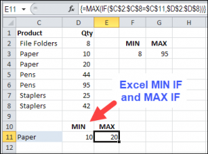
In this example, we want to see the MIN and MAX for a specific product. There is a SUMIF function and a COUNTIF function, but no MINIF or MAXIF.
- [Update]: In Excel 2019, and Excel for Office 365, you can use the new MINIFS and MAXIFS functions. There is more information on the MIN and MAX page on my Contextures site.
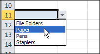
So, we’ll have to create our own MINIF formula, using MIN and IF. I’ve selected a product in cell C11, and the formula will be built in cell D11.
To make it easy to select a product, I created a drop down list of product names, by using data validation.
NOTE: You can also calculate MIN IF and MAX IF with Multiple Criteria
MIN IF Formula
The formula starts with the MIN and IF functions, and their opening brackets:
=MIN(IF(
Next, we want to find the rows where the product name matches the product in C11:
- Select C2:C8, where the product names are listed
- Type an = sign
- Click on cell C11
=MIN(IF(C2:C8=C11

Next, select D2:D8, where the quantities are listed. If the product name matches, we want to check the product quantity
=MIN(IF(C2:C8=C11,D2:D8

To finish the formula:
- Type two closing brackets
- Then press Ctrl+Shift+Enter to array-enter the formula.
=MIN(IF(C2:C8=C11,D2:D8))

NOTE: If you plan to copy this formula down a column, use absolute references to the product and quantity ranges:
=MIN(IF($C$2:$C$8=C11,$D$2:$D$8))
Array Entered Formula
If you select cell D11, and look at the formula in the Formula Bar, there are curly brackets at the start and end of the formula. Those were automatically added, because the formula was array-entered (Ctrl + Shift + Enter).
If you don’t see those curly brackets, you pressed Enter, instead of Ctrl + Shift + Enter.
To fix the formula:
- Click in the formula bar (it doesn’t matter where you click within the formula)
- Press Ctrl + Shift + Enter.

Create a MAXIF Formula
To find the maximum quantity for a specific product, use MAX instead of MIN.
=MAX(IF(C2:C8=C11,D2:D8))
or use absolute references for the product and quantity ranges:
=MAX(IF($C$2:$C$8=C11,$D$2:$D$8))
And remember to press Ctrl+Shift+Enter

Multiple Criteria for MIN IF or MAX IF
These formulas have only one criterion — the product name. If you’re ready for the next challenge, you can also calculate MIN IF and MAX IF with Multiple Criteria
- [Update]: In Excel 2019, and Excel 365, you can use the new MINIFS and MAXIFS functions. For more information, go to the MIN and MAX page on my Contextures site.
Watch the MIN IF or MAX IF Video
To see the steps for creating MIN IF and MAX IF formulas, watch this short Excel video tutorial. The sample file for this video can be downloaded from my Contextures website, on the MIN and MAX page.
Your browser can’t show this frame. Here is a link to the page
________________________
________________
In Excel, we can’t simply use the default MAX function with a condition (unless you are using Microsoft Office 365).
But the thing is if want to get maximum value from a range using a specific condition you need a MAX IF formula.
So what’s the point?
You can combine MAX and IF to create a formula that can help you to get the max value from a range using specific criteria.
In short: MAXIF is an array formula that you can use to find the max value from a range using criteria. But here’s the kicker: In this post, I’m gonna share with you different ways to use the MAXIF formula.
Apply MAX IF Formula
Let’s take an example of the below data where you have month-wise, week-wise, and date-wise sales quantity.

Now from this data, you need to get the max sales quantity for a particular month. For example, “Jan” and for this, the formula will be:
=MAX(IF(A2:A367="Jan",D2:D367))And you need to enter it as an array formula by using ctrl + shift + enter.
{=MAX(IF(A2:A367="Jan",D2:D367))}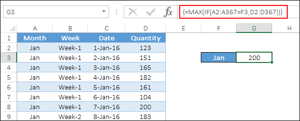
When you enter it, it will return 200 which is the highest sales value in the month of Jan on 07-Jan-2016.
How does this work
To understand the working of max if you need to split it into three parts.

Please take note that you have entered it as an array formula.
First of all, you have created a logical test in the IF function to match the entire month column with the criteria. And, it has returned an array where match values are TRUE and all others are FALSE.

Second, in the IF function, you have specified the sales quantity column for the TRUE values and that’s why it has returned sales quantity only for the TRUE.

Third, the MAX function will simply return the highest number from this array which is the highest sales quantity for the month of Jan. Just like this formula hack here I’ve listed some of the others which you must read and learn.
- SUMIFOR in Excel
- RANKIF in Excel
I am sure at this point you are thinking that how we can use more than one condition in max if. And that’s a smart thought.
In the real world of data, there is a huge possibility that we need to use multiple criteria to get the highest value. Let’s continue with the previous example.
Let’s say, instead of the highest sales value from the month of Jan, you need to get the highest sales for week 2 of Jan.
So, here you have two different conditions, the month is Jan and the week is the 2nd. And, the formula will be:
=MAX(IF(A2:A367=F5,IF(B2:B367=G5,D2:D367),))And, when you enter it as an array:
{=MAX(IF(A2:A367=F5,IF(B2:B367=G5,D2:D367),))}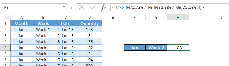
How does this work
Here we have used nested IF to test more than one logic. One is for the month and the second is for the week.
So it returns an array where you have sales quantity only where the month is Jan and the week is the 2nd.

And in the end, max returns the max value from that array.
MAX IF without an Array
Arrays are powerful but not everyone wants to use them. And, you have an option not to use an array in max if.
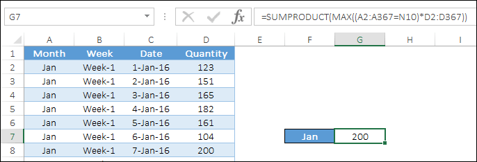
So for this, you can use the SUMPRODUCT function because it can help you to use an array without applying the actual array formula. And the formula will be:
=SUMPRODUCT(MAX((A2:A367="Jan")*D2:D367))So when you insert this formula you don’t need to use ctrl + shift + enter.
How does this work
Again we need to split this formula into three different parts to understand it. In the first part, you have compared the month column with the criteria and it has returned an array with TRUE where criteria matched, else FALSE.

After that, you have multiplied that array with the sales quantity column which returns an array where you have sales quantity instead of TRUE. In the end, the MAX function has returned the highest value from that array which is your highest sales quantity.
This entire formula, sumproduct has the major role to allow you to use an array without entering an actual array formula.
Conclusion
Getting the max value based on criteria is what we often need to do. And using this technique of max if the formula you can do it with no effort.
All the methods which you have learned above have different applications according to the situation. I hope this formula tip will help you to get better at Excel. But now, tell me one thing.
Which one do you really like, an array or without an array?
Please share your views with me in the comment section. I’d love to hear from you, and please, don’t forget to share this post with your friends, I am sure they will appreciate it.