
You can work with a matrix in the Excel just like with a range. That is, a set of adjacent cells occupying a rectangular area.
The matrix address is the upper left and right lower cell of the range indicated by the colon.
Array formulas
Building a matrix of Excel tools in most cases requires the use of appropriate arrays. Their main difference is that the result is not one value but a data set (a range of numbers).
The procedure for applying the data set formula:
- Select the range where the result of the formula action should appear.
- Enter the formula (starting with the sign «=»).
- Press the kea combination Ctrl + Shift + Enter.
The data set formula in curly brackets is displayed in the formula bar.
Select the entire range and perform the appropriate actions to change or delete a data set formula. The same combination is used (Ctrl + Shift + Enter) to enter changes. Part of the data set cannot be changed.
Matrix operations in Excel
You can perform such operations with matrices in Excel as transposition, addition, multiplication by number/array; finding the inverse matrix and its determinant.
Transpose the matrices
Transposing the matrix is an act of changing the rows and columns in places.
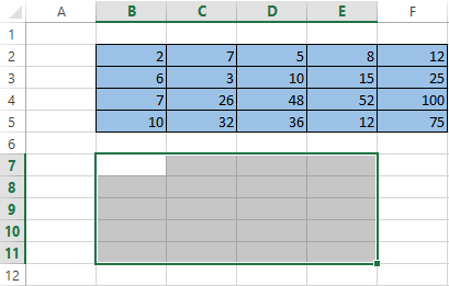
First, note the empty range where we transpose the matrix. There are 4 lines in the original table and the range for the transposition should have 4 columns. For 5 columns there are should be five lines in an empty area, etc.
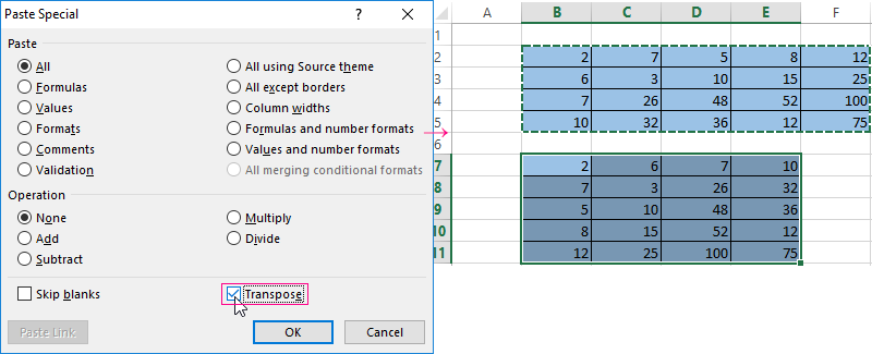
- Method #1. Select the original data array. Click «copy». Select an empty range. Expand the Paste button. Open the «Paste Special» menu (CTRL+ALT+V). Mark «Transpose» operation. Close the dialog by clicking OK.
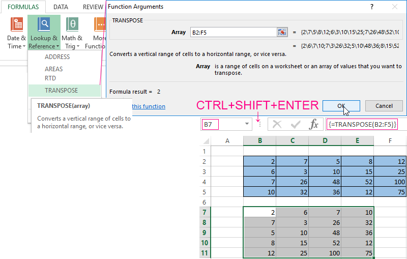
- Method #2. Select the range B7:E11 with active cell B7 in the upper left corner of the empty range. Select function: «FORMULAS»-«Lookup and Reference»-«TRANSPOSE». The argument is a range with the original array data. Click OK. Now the function produces an error. Select the entire range where you want to transpose the matrix. Press the F2 (go to the formula editing mode). Press the key combination Ctrl + Shift + Enter.
The advantage of the second method: the transposed matrix automatically changes while making changes to the original.
Addition of a matrices
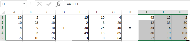
You can sum up matrices with the same number of elements. The number of rows and columns of the first range should be equal to the number of rows and columns of the second range.
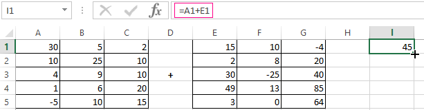
In the first cell of the resulting matrix you need to enter a formula of the next form: = the first element of the first array + the first element of the second: (=A1+E1). Press Enter and stretch the formula to the full range.
Matrices multiplication in Excel
The task is next:
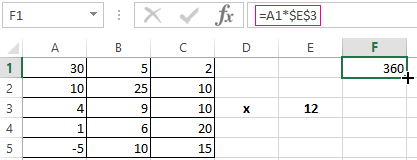
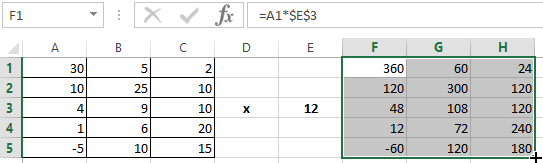
To multiply a matrix by a number you need to multiply each of its elements by this number. The formula in Excel: =A1*$E$3 ( a reference to a cell with a number must be absolute).
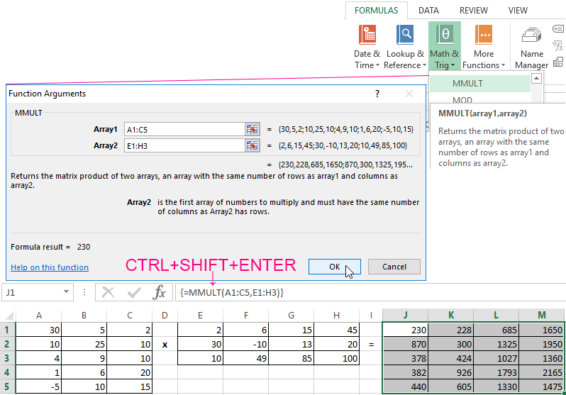
Let’s multiply the matrix with different ranges. It’s possible only to find the product of matrices if the number of columns of the first matrix is equal to the number of rows of the second one.
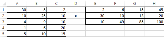
In the resulting matrix, the number of rows is equal to the number of rows of the first array, and the number of columns is equal to the number of columns of the second.
For convenience, we select the range where the multiplication results will be placed. We make the first cell of the resulting field active. Then select: «FORMULAS»-«Math and Trig»-«MMULT» We introduce the formula: = =MMULT(A1:C5,E1:H3). Enter as an array formula (CTRL+SHIFT+Enter).
The inverse matrices in Excel
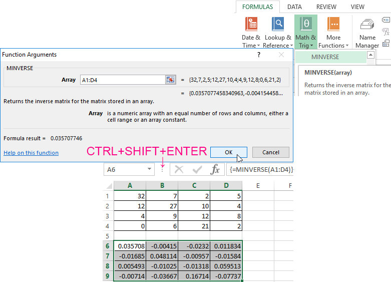
It makes sense to find it if we are dealing with a square matrix (the number of rows and columns is the same).
The dimension of the inverse matrix corresponds to the size of the original. We use: «FORMULAS»-«Math and Trig»-«MINVERSE» function in Excel.
Select the first cell of the empty range for the inverse matrix. We introduce the formula «= MINVERSE(A1:D4)» as a data set function. The only argument is the range with the original. We got the inverse array in Excel:
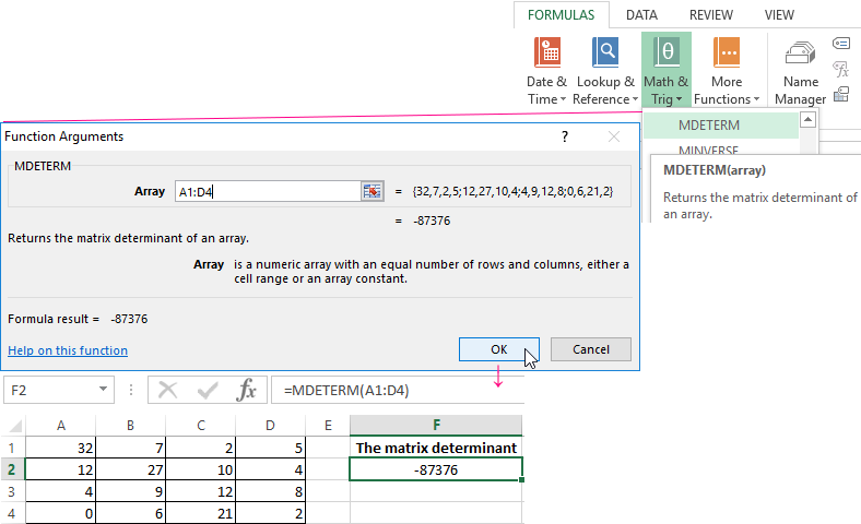
Finding the matrices determinant
This is one single number that is found for a square matrix. We use: «FORMULAS»-«Math and Trig»-«MDETERM» function.
We put the cursor in any cell of the open sheet. Enter the formula: =MOPRED(A1:D4).
Thus, we performed actions with the matrixes using the built-in Excel features.
Содержание
- Excel
- Contents:
- Introduction
- Named Ranges
- Matrix Operations in Excel
- Matrix Addition
- Matrix Subtraction
- Using Matrices with Scalars
- Matrix Multiplication
- Transposition
- Matrix Inversion
- Combining Matrix Operations
- Working with a matrix in Power View
- Functions for working with a matrix in Excel
- Array formulas
- Matrix operations in Excel
- Transpose the matrices
- Addition of a matrices
- Matrices multiplication in Excel
- The inverse matrices in Excel
- Finding the matrices determinant
Excel
Contents:
Introduction
Microsoft’s Excel spreadsheet program provides an alternative environment for many of the computations required for Macro-Investment Analysis. Its ubiquity and ease of use are among its more attractive features. However, spreadsheets are notoriously dangerous, since the underlying logic of a set of calculations is usually contained in formulas scattered around a sheet (or sheets). Worse yet, the formulas are usually hidden from sight, behind the numbers representing the results of their calculations. These disadvantages loom especially large when an environment is to be chosen primarily as a means of communication. For our purposes, languages such as MATLAB are superior to a spreadsheet environment — Excel or any other.
The situation is not, however, as bleak as it once was. Since the introduction of version 5.0, Excel has included a full programming language that allows for structured, documented, and readable sets of commands. Formally, it is a version of Microsoft’s Visual Basic for Applications, but we will use the simpler form: Visual Basic or to be even more succinct: VB.
In Excel, VB procedures are called Macros , but this is far too humble a term for perfectly respectable programs and we will resist its use except when absolutely necessary.
Will will not cover Visual Basic, since it is a complex programming language that requires an extensive treatise. Suffice it to say that it provides an alternative to MATLAB and other languages for preparing investment application programs.
Here we concentrate on a a discussion of matrix operations in the standard Excel spreadsheet environment. The treatment will be cursory, at best since Excel is far too complex to cover in any detail in this exposition. Our goal is only to suggest ways in which it can be used by the Analyst for matrix operations.
Named Ranges
Many Excel formulas require the specification of one or more ranges of cells as arguments. In many cases the easiest way to indicate such a range is to select it using keystrokes and/or a mouse as the formula is typed. For clarity, we adopt an alternative approach, using only named ranges in our formulas and statements. Since names remain with the formulas and statements, it is easy to change the physical range of cells to which a name applies whenever results are desired for a different range of inputs. Perhaps more important, the use of appropriate range names can greatly improve the readability of a set of formulas or statements.
The safest way to assign a name to a range of cells is to first select it, then choose Insert Name Define from the menu, followed by the desired name. Be certain to avoid names that look like cell locations or combinations of them (e.g. A22). In Excel, range names are not case sensitive. Thus Prices, prices and PRICES are considered the same name.
To select a named range, choose Edit Go to (or the equivalent key), followed by the range name. Alternatively, use the drop-down list of names located just above and to the left of the spreadsheet. When a named range is selected, the name will appear in the window for this list. (In fact, you can name ranges by selecting them, then typing the name in this box; however, this sometimes allows conflicts to creep in and should be avoided).
Once you have named a range, you may use it in any formula that allows for a range as an argument. As indicated earlier, we will always choose this alternative.
Matrix Operations in Excel
Unbeknownst to many users, Excel can do matrix operations very efficiently, either directly, or through the use of matrix functions. Microsoft prefers to use the term «Array» to «Matrix», so most references in their manuals and help system can be found under the former term.
Key to understanding the use of matrix operations in Excel is the concept of the Matrix (Array) formula. Such a formula uses matrix operations and returns a result that can be a matrix, a vector, or a scalar, depending on the computations involved. Whatever the result may be, an area on the spreadsheet of precisely the correct size must be selected before the formula is typed in (otherwise you will either lose some of the answer or get added and possibly confusing information).
After typing such a formula, you «enter» it with three keys pressed at once: CTRL, SHIFT and ENTER. This indicates that a matrix (array) result really is desired. It also designates the entire selected range as the desired location for the answer. To modify or delete the formula, select the entire region beforehand.
When matrix computations are performed in this way, the «result areas» will be updated immediately whenever any of the numbers in the «input areas» change (unless automatic recomputation has been turned off). This can be a great help when one wishes to evaluate the effects of changes in assumptions, initial conditions, etc.. This feature, coupled with the ability to see matrices, complete with identification of the rows and columns (i.e. in the form that we have termed tables), will often make the spreadsheet environment the preferred choice for computation, if not for communication.
In Excel, some matrix operations are performed automatically, using standard operators (as in MATLAB). Others require the use of matrix functions. We treat each below.
Matrix Addition
Assume that Holdings_1 and Holdings_2 are two ranges of the same size (say, <20*1>) containing the holdings of mutual funds in two accounts. To create a vector with the total holdings of both accounts, select an empty <20*1>range on the sheet, type in the formula:
then press CTRL-SHIFT-ENTER. As a matter of good practice, you might wish to name the resultant range (e.g. Tot_Holdings) for future reference.
Any two matrices of the same size can be added in this manner, with the result placed in a range of the same size.
Matrix Subtraction
Not surprisingly, a matrix can be subtracted from one of the same size in a manner analogous to that of addition. For example to find the holdings of account 2, you could use the formula:
Using Matrices with Scalars
To add a constant to every element of a matrix, simply include it in a formula, as in:
You can also subtract a constant from every element or multiply or divide every element by a constant. For example:
Matrix Multiplication
To multiply two matrices, use the MMULT function. Thus, if prices and holdings are compatible for multiplication, you could compute the value of a portfolio with the formula:
Transposition
If a matrix is not turned in the right direction, simply use the TRANSPOSE function. Thus if prices is a <20*1>vector and holdings is also, you could use the formula:
to produce the value of the portfolio.
As is often the case, there is another way to do the same thing in Excel. The (non-matrix) function SUMPRODUCT produces the sum of the products of the elements in two vectors of equal dimensions. Thus if prices and holdings are both <20*1>, you could compute the value of the portfolio with the formula:
Note that to enter this formula, only the ENTER key need be pressed.
The provision of alternative methods for accomplishing a given type of calculation endears Excel to many users, especially those who grew up with prior versions. But it tends to frustrate those who yearn, perhaps quixotically, for a simple, yet powerful computing environment.
Matrix Inversion
To produce the inverse of a matrix, use the MINVERSE function, as in:
Of course the matrix in the named range must be square and invertable.
Combining Matrix Operations
In Excel, as in MATLAB, you may combine matrix operations in a single formula. Remember, however, that everything must conform, that the output range should be the correct size for the final result, and that you must press CTRL-SHIFT-ENTER to enter the formula in the output range. As in more mundane formulas, it never hurts to include sufficient parentheses to remove any possible ambiguity concerning your desires.
Источник
Working with a matrix in Power View
Important: In Excel for Microsoft 365 and Excel 2021, Power View is removed on October 12, 2021. As an alternative, you can use the interactive visual experience provided by Power BI Desktop, which you can download for free. You can also easily Import Excel workbooks into Power BI Desktop.

A matrix is a type of visualization that is similar to a table in that it is made up of rows and columns. However, a matrix can be collapsed and expanded by rows and/or columns. If it contains a hierarchy, you can drill down/drill up. It can display totals and subtotals by columns and/or rows. And a matrix can display data without repeating values. For example, visualizing data about Olympic sports, disciplines, and events:
On the left, the table lists the sport and discipline for each and every event.
On the right, the matrix lists each sport and discipline only once.

To create a matrix, you start with a table and convert it to a matrix.
On the Design tab > Switch Visualizations > Table > Matrix.
By default a matrix has totals, and subtotals for the groups, but you can turn them off.
On the Design tab > Options > Totals.
To add column groups, drag a field to the Column Groups box.
Tip: If you don’t see the Column Groups box, make sure Matrix is selected on the Design tab.
Источник
Functions for working with a matrix in Excel
You can work with a matrix in the Excel just like with a range. That is, a set of adjacent cells occupying a rectangular area.
The matrix address is the upper left and right lower cell of the range indicated by the colon.
Array formulas
Building a matrix of Excel tools in most cases requires the use of appropriate arrays. Their main difference is that the result is not one value but a data set (a range of numbers).
The procedure for applying the data set formula:
- Select the range where the result of the formula action should appear.
- Enter the formula (starting with the sign «=»).
- Press the kea combination Ctrl + Shift + Enter.
The data set formula in curly brackets is displayed in the formula bar.
Select the entire range and perform the appropriate actions to change or delete a data set formula. The same combination is used (Ctrl + Shift + Enter) to enter changes. Part of the data set cannot be changed.
Matrix operations in Excel
You can perform such operations with matrices in Excel as transposition, addition, multiplication by number/array; finding the inverse matrix and its determinant.
Transpose the matrices
Transposing the matrix is an act of changing the rows and columns in places.
First, note the empty range where we transpose the matrix. There are 4 lines in the original table and the range for the transposition should have 4 columns. For 5 columns there are should be five lines in an empty area, etc.
- Method #1. Select the original data array. Click «copy». Select an empty range. Expand the Paste button. Open the «Paste Special» menu (CTRL+ALT+V). Mark «Transpose» operation. Close the dialog by clicking OK.

- Method #2. Select the range B7:E11 with active cell B7 in the upper left corner of the empty range. Select function: «FORMULAS»-«Lookup and Reference»-«TRANSPOSE». The argument is a range with the original array data. Click OK. Now the function produces an error. Select the entire range where you want to transpose the matrix. Press the F2 (go to the formula editing mode). Press the key combination Ctrl + Shift + Enter.
The advantage of the second method: the transposed matrix automatically changes while making changes to the original.
Addition of a matrices
You can sum up matrices with the same number of elements. The number of rows and columns of the first range should be equal to the number of rows and columns of the second range.
In the first cell of the resulting matrix you need to enter a formula of the next form: = the first element of the first array + the first element of the second: (=A1+E1). Press Enter and stretch the formula to the full range.
Matrices multiplication in Excel
The task is next:
To multiply a matrix by a number you need to multiply each of its elements by this number. The formula in Excel: =A1*$E$3 ( a reference to a cell with a number must be absolute).
Let’s multiply the matrix with different ranges. It’s possible only to find the product of matrices if the number of columns of the first matrix is equal to the number of rows of the second one.
In the resulting matrix, the number of rows is equal to the number of rows of the first array, and the number of columns is equal to the number of columns of the second.
For convenience, we select the range where the multiplication results will be placed. We make the first cell of the resulting field active. Then select: «FORMULAS»-«Math and Trig»-«MMULT» We introduce the formula: = =MMULT(A1:C5,E1:H3). Enter as an array formula (CTRL+SHIFT+Enter).
The inverse matrices in Excel
It makes sense to find it if we are dealing with a square matrix (the number of rows and columns is the same).
The dimension of the inverse matrix corresponds to the size of the original. We use: «FORMULAS»-«Math and Trig»-«MINVERSE» function in Excel.
Select the first cell of the empty range for the inverse matrix. We introduce the formula «= MINVERSE(A1:D4)» as a data set function. The only argument is the range with the original. We got the inverse array in Excel:
Finding the matrices determinant
This is one single number that is found for a square matrix. We use: «FORMULAS»-«Math and Trig»-«MDETERM» function.
We put the cursor in any cell of the open sheet. Enter the formula: =MOPRED(A1:D4).
Thus, we performed actions with the matrixes using the built-in Excel features.
Источник
Под матрицей подразумевается набор ячеек, расположенных непосредственно друг возле друга и которые образуют вместе прямоугольник. Не требуется особых навыков, чтобы выполнять различные действия с матрицей, достаточно тех же, какие используются во время работы с классическим диапазоном.
Каждая матрица имеет свой адрес, записывающийся аналогичным диапазону способом. Первая составная часть – первая ячейка диапазона (расположенная в верхнем левом углу), а второй – последняя ячейка, которая находится в нижнем правом углу.
Содержание
- Формулы массива
- Что можно делать с матрицами
- Транспонирование
- Сложение
- Умножение
- Обратная матрица
- Поиск определителя матрицы
- Несколько примеров
- Умножение и деление
- Метод 1
- Метод 2
- Сложение и вычитание
- Метод 1
- Метод 2
- Пример транспонирования матрицы
- Поиск обратной матрицы
- Выводы
Формулы массива
В подавляющем количестве задач при работе с массивами (а матрицы и являются таковыми) используются формулы соответствующего типа. Базовое их отличие от обычных заключается в том, что последние выводят всего одно значение. Для применения формулы массива необходимо осуществить несколько действий:
- Выделить набор ячеек, где будут выводиться значения.
- Непосредственно введение формулы.
- Нажатие последовательности клавиш Ctrl + Shift + Ввод.
После осуществления этих простых действий в поле ввода отображается формула массива. Ее можно отличить от обычной по фигурным скобкам.
Для редактирования, удаления формул массива, надо выделить требуемый диапазон и сделать то, что нужно. Чтобы редактировать матрицу, нужно использовать ту же комбинацию, что и для ее создания. При этом нет возможности редактировать отдельный элемент массива.
Что можно делать с матрицами
В целом, есть огромное количество действий, применение которых возможно для матриц. Давайте каждое из них рассмотрим более подробно.
Транспонирование
Многие люди не понимают значения этого термина. Представьте, что вам нужно поменять строки и колонки местами. Вот это действие и называется транспонированием.
Перед тем, как это осуществить, необходимо выделить отдельную область, которая имеет такое же количество строчек, сколько столбцов есть у исходной матрицы и такое же количество столбцов. Чтобы более наглядно понять, как это работает, посмотрите на этот скриншот.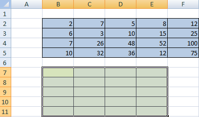
Далее есть несколько методов, как можно осуществить транспонирование.
Первый способ следующий. Для начала нужно выделить матрицу, после чего скопировать ее. Далее выделяется диапазон ячеек, куда должен быть вставлен транспонированный диапазон. Далее открывается окно «Специальная вставка».
Там есть множество операций, но нам нужно найти радиокнопку «Транспонировать». После совершения этого действия нужно подтвердить его нажатием клавиши ОК.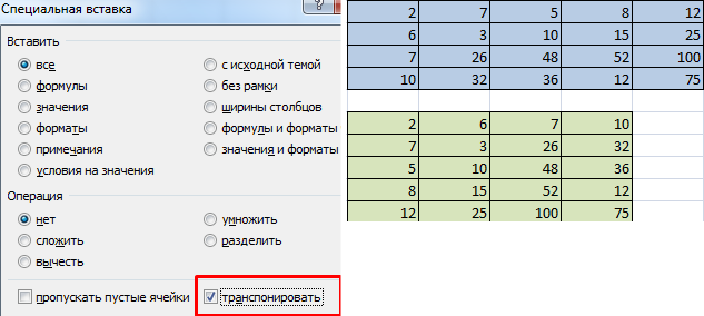
Есть еще один способ, с помощью которого можно транспонировать матрицу. Сперва надо выделить ячейку, расположенную в верхнем левом углу диапазона, отведенного под транспонированную матрицу. Далее открывается диалоговое окно с функциями, где есть функция ТРАНСП. Ниже в примере вы более подробно узнаете, как это сделать. В качестве параметра функции используется диапазон, соответствующий изначальной матрице.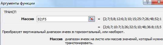
После нажатия кнопки ОК сначала будет показано, что вы допустили ошибку. Ничего в этом страшного нет. Все потому, что вставленная нами функция не определена, как формула массива. Поэтому нам нужно совершить такие действия:
- Выделить набор ячеек, отведенных под транспонированную матрицу.
- Нажать клавишу F2.
- Нажать на горячие клавиши Ctrl + Shift + Enter.
Главное достоинство метода заключается в способности транспонированной матрицы сразу корректировать содержащуюся в ней информацию, как только вносятся данные в изначальную. Поэтому рекомендуется использовать именно данный способ.
Сложение
Эта операция возможна лишь применительно к тем диапазонам, количество элементов которых такое же самое. Проще говоря, у каждой из матриц, с которыми пользователь собирается работать, должны быть одинаковые размеры. И приводим скриншот для наглядности.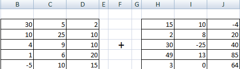
В матрице, которая должна получиться, нужно выделить первую ячейку и ввести такую формулу.
=Первый элемент первой матрицы + Первый элемент второй матрицы
Далее подтверждаем ввод формулы с помощью клавиши Enter и используем автозаполнение (квадратик в правом нижнем углу), чтобы скопировать все значения на новую матрицу.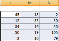
Умножение
Предположим, у нас есть такая таблица, которую следует умножить на 12.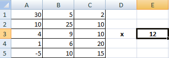
Догадливый читатель может легко понять, что метод очень похож на предыдущий. То есть, каждая из ячеек матрицы 1 должна умножаться на 12, чтобы в итоговой матрице каждая ячейка содержала значение, умноженное на этот коэффициент.
При этом важно указывать абсолютные ссылки на ячейки.
Итого, получится такая формула.
=A1*$E$3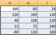
Дальше методика аналогична предыдущей. Нужно это значение растянуть на необходимое количество ячеек.
Предположим, что необходимо перемножить матрицы между собой. Но есть лишь одно условие, при котором это возможно. Надо, чтобы количество столбцов и строк у двух диапазонов было зеркально одинаковое. То есть, сколько столбцов, столько и строк.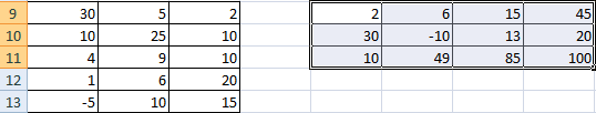
Чтобы было более удобно, нами выделен диапазон с результирующей матрицей. Надо переместить курсор на ячейку в верхнем левом углу и ввести такую формулу =МУМНОЖ(А9:С13;Е9:H11). Не стоит забыть нажать Ctrl + Shift + Enter.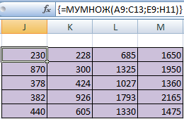
Обратная матрица
Если наш диапазон имеет квадратную форму (то есть, количество ячеек по горизонтали и вертикали одинаковое), то тогда получится найти обратную матрицу, если в этом есть такая необходимость. Ее величина будет аналогичной исходной. Для этого используется функция МОБР.
Для начала следует выделить первую ячейку матрицы, в какую будет вставляться обратная. Туда вводится формула =МОБР(A1:A4). В аргументе указывается диапазон, для какого нам надо создать обратную матрицу. Осталось только нажать Ctrl + Shift + Enter, и готово.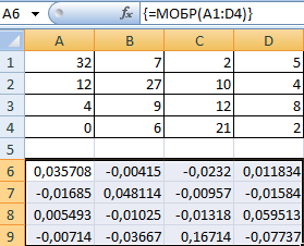
Поиск определителя матрицы
Под определителем подразумевается число, находящееся матрицы квадратной формы. Чтобы осуществить поиск определителя матрицы, существует функция – МОПРЕД.
Для начала ставится курсор в какой-угодно ячейке. Далее мы вводим =МОПРЕД(A1:D4)
Несколько примеров
Давайте для наглядности рассмотрим некоторые примеры операций, которые можно осуществлять с матрицами в Excel.
Умножение и деление
Метод 1
Предположим, у нас есть матрица A, имеющая три ячейки в высоту и четыре – в ширину. Также есть число k, которое записывается в другой ячейке. После выполнения операции умножения матрицы на число появится диапазон значений, имеющий аналогичные размеры, но каждая ее часть умножается на k.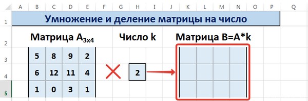
Диапазон B3:E5 – это исходная матрица, которая будет умножаться на число k, которое в свою очередь расположено в ячейке H4. Результирующая матрица будет находиться в диапазоне K3:N5. Исходная матрица будет называться A, а результирующая – B. Последняя образуется путем умножения матрицы А на число k.
Далее вводится =B3*$H$4 в ячейку K3, где В3 — элемент A11 матрицы А.
Не стоит забывать о том, ячейку H4, где указано число k необходимо вводить в формулу с помощью абсолютной ссылки. Иначе значение будет изменяться при копировании массива, и результирующая матрица потеряет работоспособность.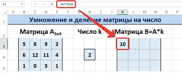
Далее маркер автозаполнения (тот самый квадратик в правом нижнем углу) используется для того, чтобы скопировать значение, полученное в ячейке K3, во все другие ячейки этого диапазона.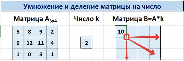
Вот у нас и получилось умножить матрицу A на определенное число и получить на выходе матрицу B.
Деление осуществляется аналогичным образом. Только вводить нужно формулу деления. В нашем случае это =B3/$H$4.
Метод 2
Итак, основное отличие этого метода в том, в качетве результата выдается массив данных, поэтому нужно применить формулу массива, чтобы заполнить весь набор ячеек.
Необходимо выделить результирующий диапазон, ввести знак равно (=), выделить набор ячеек, с соответствующими первой матрице размерами, нажать на звездочку. Далее выделяем ячейку с числом k. Ну и чтобы подтвердить свои действия, надо нажать на вышеуказанную комбинацию клавиш. Ура, весь диапазон заполняется.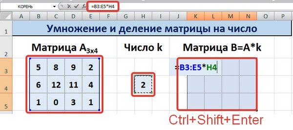
Деление осуществляется аналогичным образом, только знак * нужно заменить на /.
Сложение и вычитание
Давайте опишем несколько практических примеров использования методов сложения и вычитания на практике.
Метод 1
Не стоит забывать, что возможно сложение лишь тех матриц, размеры которых одинаковые. В результирующем диапазоне все ячейки заполняются значением, являющим собой сумму аналогичных ячеек исходных матриц.
Предположим, у нас есть две матрицы, имеющие размеры 3х4. Чтобы вычислить сумму, следет в ячейку N3 вставить такую формулу:
=B3+H3
Тут каждый элемент являет собой первую ячейку матриц, которые мы собрались складывать. Важно, чтобы ссылки были относительными, поскольку если использовать абсолютные, не будут отображаться правильные данные.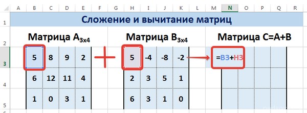
Далее, аналогично умножению, с помощью маркера автозаполнения распространяем формулу на все ячейки результирующей матрицы.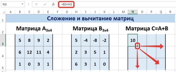
Вычитание осуществляется аналогично, за тем лишь исключением, что используется знак вычитания (-), а не сложения.
Метод 2
Аналогично методу сложения и вычитание двух матриц, этот способ подразумевает использование формулы массива. Следовательно, в качестве ее результата будет выдаваться сразу набор значений. Поэтому нельзя редактировать или удалять какие-то элементы.
Сперва надо выделить диапазон, отделенный под результирующую матрицу, а потом нажать на «=». Затем надо указать первый параметр формулы в виде диапазона матрицы А, нажать на знак + и записать второй параметр в виде диапазона, соответствующему матрице B. Подтверждаем свои действия нажатием комбинации Ctrl + Shift + Enter. Все, теперь вся результирующая матрица заполнена значениями.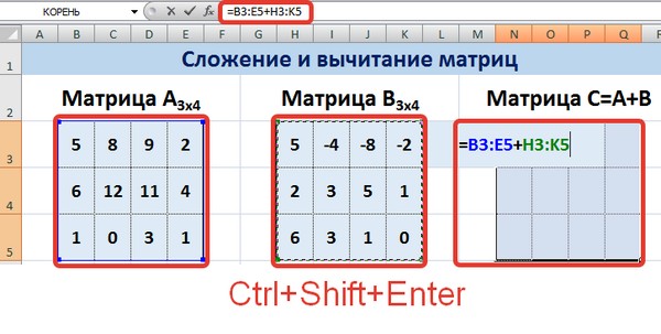
Пример транспонирования матрицы
Допустим, нам надо создать матрицу АТ из матрицы А, которая у нас есть изначально методом транспонирования. Последняя имеет, уже по традиции, размеры 3х4. Для этого будем использовать функцию =ТРАНСП().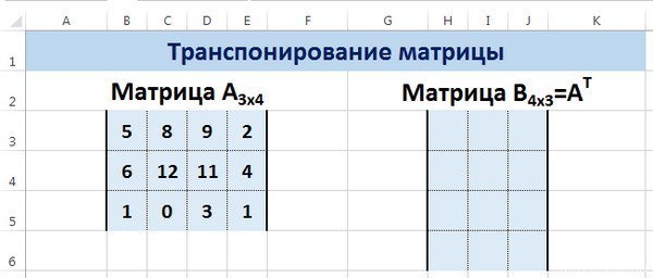
Выделяем диапазон для ячеек матрицы АТ.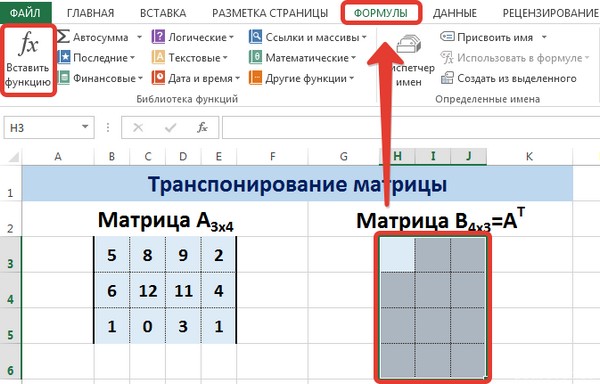
Для этого надо перейти на вкладку «Формулы», где выбрать опцию «Вставить функцию», там найти категорию «Ссылки и массивы» и найти функцию ТРАНСП. После этого свои действия подтверждаются кнопкой ОК.
Далее переходим в окно «Аргументы функции», где вводится диапазон B3:E5, который повторяет матрицу А. Далее надо нажать Shift + Ctrl, после чего кликнуть «ОК».
Важно. Нужно не лениться нажимать эти горячие клавиши, потому что в ином случае будет рассчитано только значение первой ячейки диапазона матрицы АТ.
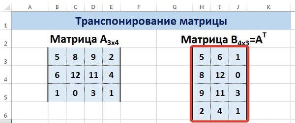
В результате, у нас получается такая транспонированная таблица, которая изменяет свои значения вслед за исходной.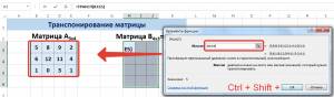
Поиск обратной матрицы
Предположим, у нас есть матрица А, которая имеет размеры 3х3 ячеек. Мы знаем, что для поиска обратной матрицы необходимо использовать функцию =МОБР().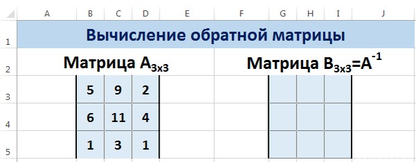
Теперь опишем, как это делать на практике. Сначала необходимо выделить диапазон G3:I5 (там будет располагаться обратная матрица). Необходимо найти на вкладке «Формулы» пункт «Вставить функцию».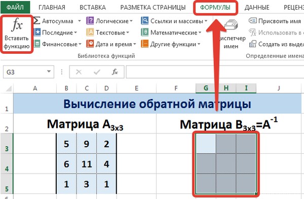
Откроется диалог «Вставка функции», где нужно выбрать категорию «Математические». И там в перечне будет функция МОБР. После того, как мы ее выберем, нужно нажать на клавишу ОК. Далее появляется диалоговое окно «Аргументы функции», в котором записываем диапазон B3:D5, который соответствует матрице А. Далее действия аналогичные транспонированию. Нужно нажать на комбинацию клавиш Shift + Ctrl и нажать ОК.
Выводы
Мы разобрали некоторые примеры, как можно работать с матрицами в Excel, а также описали теорию. Оказывается, что это не так страшно, как может показаться на первый взгляд, не так ли? Это только звучит непонятно, но на деле с матрицами среднестатистическому пользователю приходится иметь дело каждый день. Они могут использоваться почти для любой таблицы, где есть сравнительно небольшое количество данных. И теперь вы знаете, как можно себе упростить жизнь в работе с ними.
Оцените качество статьи. Нам важно ваше мнение:
What is Matrix Multiplication on Excel?
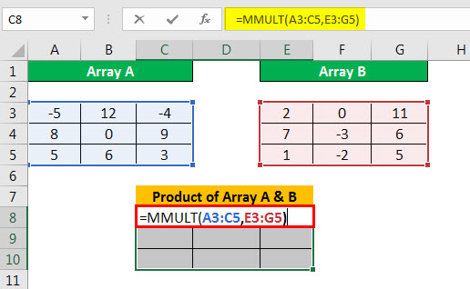
In Excel, we have an inbuilt function for matrix multiplication. It is an MMULT function. It takes two arrays as an argument and returns the product of two arrays, given that both the arrays should have the same number of rows and columns.
Explanation
Matrix multiplication is one of the useful features of excelThe top features of MS excel are — Shortcut keys, Summation of values, Data filtration, Paste special, Insert random numbers, Goal seek analysis tool, Insert serial numbers etc.
read more presented to do mathematical operations. It helps to gain the product of two matrices. The matrices that want to multiply have a certain number of rows and columns to present the data. The resulting matrix size is taken from the number of rows of the first array and the number of columns of the second array. However, there is a condition to matrix multiplication. The number of columns in the first matrix should equal the number of rows in the second matrix.
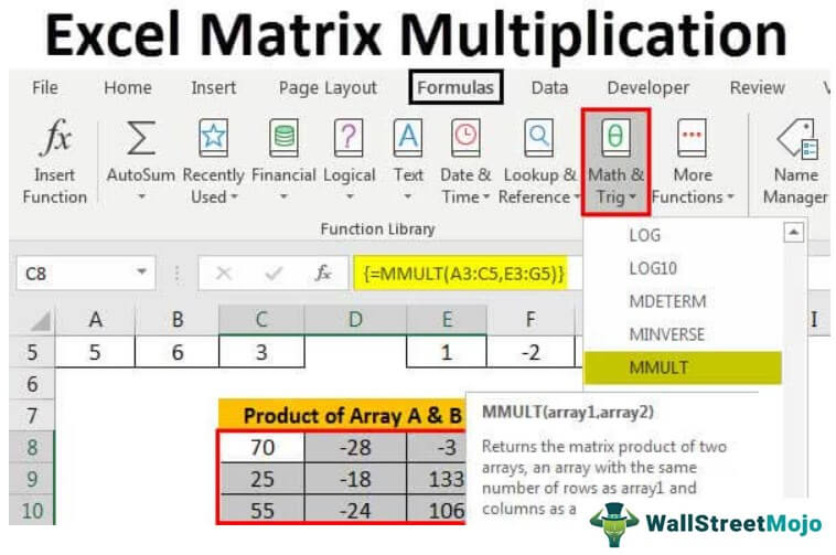
The predefined MMULT function presented in the Excel software is used to perform the matrix multiplication. Excel matrix multiplication reduces a lot of time incurred in manually calculating the product of matrices.
In general, we can do matrix multiplication in two ways. First, simple scalar multiplication is performed using the basic arithmetic operations. Second, advanced matrix multiplication is managed with the help of array function in excelArray formulas are extremely helpful and powerful formulas that are used in Excel to execute some of the most complex calculations. There are two types of array formulas: one that returns a single result and the other that returns multiple results.read more.
The Excel formula used for multiplicationMultiplication in excel is performed by entering the comparison operator “equal to” (=), followed by the first number, the “asterisk” (*), and the second number.read more is entered in two ways, including manually typing the MMULT function after the equal sign or selecting the Math and Trig function library presented under the “Formulas” tab. The mathematical function MMULT helps in returning the multiplication of two arrays. It is one of the predefined excel functionsExcel functions help the users to save time and maintain extensive worksheets. There are 100+ excel functions categorized as financial, logical, text, date and time, Lookup & Reference, Math, Statistical and Information functions.read more used in worksheets to perform calculations in a short time..
You are free to use this image on your website, templates, etc, Please provide us with an attribution linkArticle Link to be Hyperlinked
For eg:
Source: Excel Matrix Multiplication (wallstreetmojo.com)
Syntax
The required syntax that we should follow for the matrix multiplication is:
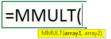
- Parameters: Array1 and array2 are the two required parameters to perform multiplication.
- Rule: Columns of array1 should be equal to rows of array2, and the size of the product must be equal to the number of rows in array1 and the number of columns in array2.
- Returns: The MMULT function generates the numbers in the product matrix. It is inserted as a formula or worksheet function in Excel calculations.
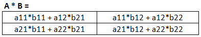
Let us consider the below image.
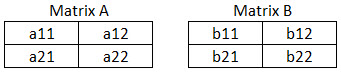
Then, the product of A*B is as follows:
How to do Matrix Multiplication in Excel? (with Examples)
Matrix multiplication in Excel has some real-time applications. There are two ways to do matrix multiplication. Below are some examples of Excel matrix multiplication.
You can download this Matrix Multiplication Excel Template here – Matrix Multiplication Excel Template
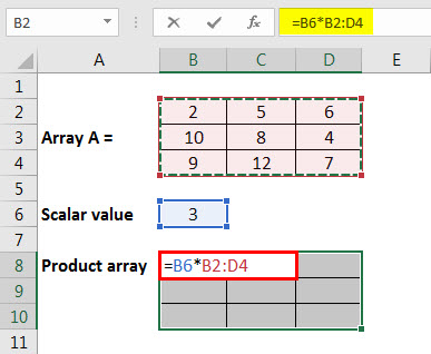
Example #1 – Multiplying a matrix with a scalar number.
Let us start.
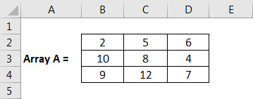
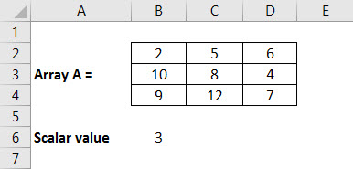
- Firstly, we must enter data into the array.

- Then, we must select a scalar value that we need to multiply with an array, i.e., 3.

- Estimate the rows and columns of the resultant array. Here, the resultant array will be of size 3 x 3.
- After that, we must select the range of cells equal to the size of the resultant array to place the result and enter the normal multiplication formula.

- On entering the formula, we must press Ctrl + Shift + Enter. Consequently, the result will be obtained, as shown below.


Example #2 – Matrix Multiplication of Two Individual Arrays
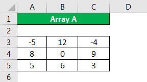
- Step 1: First, we should enter data into an array A size of 3×3.
- Step 2: Then, insert data into the second array called B size of 3×3.
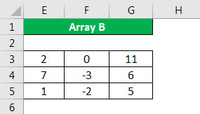
- Step 3: We need to ensure that columns of the first array are the same in size as rows of the second array.
- Step 4: Estimate the rows and columnsA cell is the intersection of rows and columns. Rows and columns make the software that is called excel. The area of excel worksheet is divided into rows and columns and at any point in time, if we want to refer a particular location of this area, we need to refer a cell.read more of the resultant array.
- Step 5: Select the range of cells equal to the size of the resultant array to place the result and enter the MMULT multiplication formula.
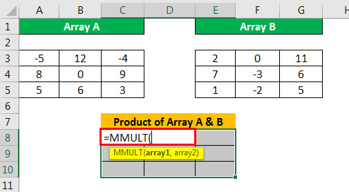
Next, we must insert the values to calculate the product of A and B.
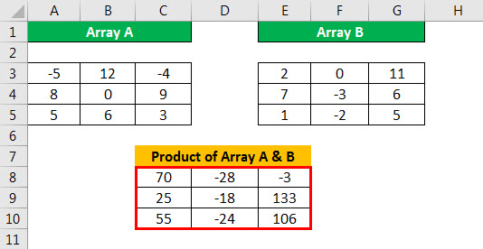
Once we enter the formula, press Ctrl + Shift + Enter to get the result. The results we can obtain by multiplying two arrays are as follows. The size of the resultant array is 3X3.
Example #3
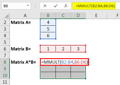
Matrix multiplication between arrays with a single row and single column. Let’s consider the elements of matrices as follows:

Matrix A is 1×3, and matrix B is 3×1. So the size of the product A*B [AB] matrix is 1×1. So, we must now insert the matrix multiplication formula in the cell.

Press the “Enter” key to get the result.

Example #4 – Matrix Multiplication Between Arrays with Single Column and a Single Row

Matrix A is 3×1, and matrix B is 1×3. The size of the product A*The B [AB] matrix is 3×3.
So, the answer will be:
Example #5 – Determining the square of a matrix using MMULT in ExcelMMULT is an in-built Math & Trigonometry function in Excel that performs matrix multiplication of 2 arrays where the columns of Array 1 are equivalent to the rows for Array 2. read more
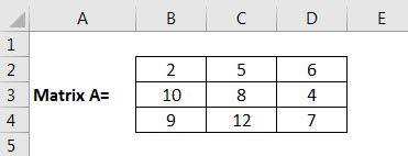
The square of matrix A is determined by multiplying A with A.
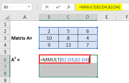
The resulting matrix is obtained as:
Things to Remember
- The number of columns presented in array1 and the number of rows present in array2 must be equal to perform matrix multiplication.
- It is hard to change the part of an array since the array is a group of elements.
- While performing an array multiplication, CTRL+SHIFT+ENTER should be used to produce all elements of the result matrix. Otherwise, it may create only a single element.
- The elements of an array should not be null, and we should not use text in matrices to avoid errors.
- The size of the product array is equal to rows of the first array and columns of the second array.
- The multiplication of A*B is not equal to the B*A in matrix multiplication.
- Multiplying a matrix with unit matrix results in the same matrix (i.e., [A]*[Unit matrix]=[A]).
Recommended Articles
This article has been a guide to Excel Matrix Multiplication. Using the scalar method and MMULT() function with examples and a downloadable Excel template, we discussed matrix multiplication in Excel. You can learn more about Excel from the following articles: –
- Excel Inverse Matrix
- Using VBA Arrays
- Using SUMPRODUCT with Multiple Criteria
- COUNTIF with Multiple Criteria
Important: In Excel for Microsoft 365 and Excel 2021, Power View is removed on October 12, 2021. As an alternative, you can use the interactive visual experience provided by Power BI Desktop, which you can download for free. You can also easily Import Excel workbooks into Power BI Desktop.
A matrix is a type of visualization that is similar to a table in that it is made up of rows and columns. However, a matrix can be collapsed and expanded by rows and/or columns. If it contains a hierarchy, you can drill down/drill up. It can display totals and subtotals by columns and/or rows. And a matrix can display data without repeating values. For example, visualizing data about Olympic sports, disciplines, and events:
On the left, the table lists the sport and discipline for each and every event.
On the right, the matrix lists each sport and discipline only once.
To create a matrix, you start with a table and convert it to a matrix.
-
On the Design tab > Switch Visualizations > Table > Matrix.
By default a matrix has totals, and subtotals for the groups, but you can turn them off.
-
On the Design tab > Options > Totals.
To add column groups, drag a field to the Column Groups box.
Tip: If you don’t see the Column Groups box, make sure Matrix is selected on the Design tab.
Top of Page
See Also
Add drill-down to a Power View chart or matrix
Charts and other visualizations in Power View
Power View: Explore, visualize, and present your data
Power View and Power Pivot videos
Tutorial: PivotTable data analysis using a Data Model in Excel 2013
Top of Page
Need more help?
Want more options?
Explore subscription benefits, browse training courses, learn how to secure your device, and more.
Communities help you ask and answer questions, give feedback, and hear from experts with rich knowledge.