
Excel for Microsoft 365 Excel for Microsoft 365 for Mac Excel for the web Excel 2021 Excel 2021 for Mac Excel 2019 Excel 2019 for Mac Excel 2016 Excel 2016 for Mac Excel 2013 Excel for Mac 2011 More…Less
This article describes the formula syntax and usage of the CEILING.MATH function in Microsoft Excel.
Description
Rounds a number up to the nearest integer or to the nearest multiple of significance.
Syntax
CEILING.MATH(number, [significance], [mode])
The CEILING.MATH function syntax has the following arguments.
-
Number Required. Number must be less than 9.99E+307 and greater than -2.229E-308.
-
Significance Optional. The multiple to which Number is to be rounded.
-
Mode Optional. For negative numbers, controls whether Number is rounded toward or away from zero.
Remarks
-
By default, significance is +1 for positive numbers and -1 for negative numbers.
-
By default, positive numbers with decimal portions are rounded up to the nearest integer. For example, 6.3 is rounded up to 7.
-
By default, negative numbers with decimal portions are rounded up (toward 0) to the nearest integer. For example, -6.7 is rounded up to -6.
-
By specifying the Significance and Mode arguments, you can change the direction of the rounding for negative numbers. For example, rounding -6.3 to a significance of 1 with a mode of 1 rounds away from 0, to -7. There are many combinations of Significance and Mode values that affect rounding of negative numbers in different ways.
-
The Mode argument does not affect positive numbers.
-
The significance argument rounds the number up to the nearest integer that is a multiple of the significance specified. The exception is where the number to be rounded is an integer. For example, for a significance of 3 the number is rounded up to the next integer that is a multiple of 3.
-
If Number divided by a Significance of 2 or greater results in a remainder, the result is rounded up.
Example
Copy the example data in the following table, and paste it in cell A1 of a new Excel worksheet. For formulas to show results, select them, press F2, and then press Enter. If you need to, you can adjust the column widths to see all the data.
|
Formula |
Description |
Result |
|
=CEILING.MATH(24.3,5) |
Rounds 24.3 up to the nearest integer that is a multiple of 5 (25). |
25 |
|
=CEILING.MATH(6.7) |
Rounds 6.7 up to the nearest integer (7). |
7 |
|
=CEILING.MATH(-8.1,2) |
Rounds -8.1 up (toward 0) to the nearest integer that is a multiple of 2 (-8). |
-8 |
|
=CEILING.MATH(-5.5,2,-1) |
Rounds -5.5 down (away from 0) to the nearest integer that is a multiple of 2 with a mode of -1, which reverses rounding direction (-6). |
-6 |
Top of Page
Need more help?
Purpose
Round a number up to nearest multiple
Usage notes
The Excel CEILING.MATH function rounds a number up to a given multiple, where multiple is provided as the significance argument. If the number is already an exact multiple, no rounding occurs and the original number is returned.
The CEILING.MATH function takes three arguments, number, significance, and mode. Number is the numeric value to round up, and is the only required argument. With no other input, CEILING.MATH will round number up to the next integer.
The significance argument is the multiple to which number should be rounded. In most cases, significance is provided as a numeric value, but CEILING.MATH can also understand time entered as text like «0:15». The default value of significance is 1.
The mode argument controls the direction negative values are rounded. By default, CEILING.MATH rounds negative values up toward zero. Setting mode to 1 or TRUE changes behavior so that negative values are rounded away from zero. The default value of mode is 0 or FALSE, so you can think of mode as a setting that means «round away from zero». Mode has no effect when number is positive.
Examples
By default, CEILING.MATH rounds to the nearest integer, using a significance of 1.
=CEILING.MATH(1.25) // returns 2
Provide a value for significance to round to a different multiple:
=CEILING.MATH(1.25,3) // returns 3
=CEILING.MATH(4.1,3) // returns 6
=CEILING.MATH(4.1,0.5) // returns 4.5
Rounding negative numbers
By default, positive numbers with decimal portions are rounded up to the nearest integer and negative numbers with decimal portions are rounded toward zero:
=CEILING.MATH(6.3) // returns 7
=CEILING.MATH(-6.3) // returns -6
Control for rounding negative numbers toward zero or away from zero is provided via the optional mode argument. Mode defaults to zero. When mode is zero, or omitted, CEILING.MATH rounds negative numbers toward zero. When mode is 1 or TRUE, CEILING.MATH rounds negative numbers away from zero. Mode has no effect on positive numbers.
=CEILING.MATH(-4.1) // returns -4
=CEILING.MATH(-4.1,1) // returns -4
=CEILING.MATH(-4.1,1,1) // returns -5
=CEILING.MATH(-4.1,1,TRUE) // returns -5
CEILING.MATH vs CEILING
The CEILING.MATH function together with the CEILING.PRECISE function replace the original CEILING function, which is now classified as a «compatibility function». The behavior is very similar, but CEILING.MATH provides explicit control over how negative numbers are rounded. CEILING.MATH differs from CEILING in these key ways:
- Rounds up to the next integer by default (i.e. significance defaults to 1)
- Provides explicit control for rounding negative numbers (toward zero, away from zero)
- Changing the sign of significance has no effect on the result; use mode instead.
Notes
- To round to the nearest multiple (up or down) see the MROUND function.
- CEILING.MATH works like CEILING, but provides control for rounding negative values.
- The mode argument has no effect on positive numbers.
- If number is an exact multiple of significance, no rounding occurs.
Содержание
- CEILING.MATH function
- Description
- Syntax
- Remarks
- Example
- Excel CEILING Function
- CEILING Function in Excel
- Syntax
- How to Use the CEILING Function in Excel?
- Example #1
- Example #2
- Example #3
- Example #4
- Things to Remember
- Recommended Articles
- CEILING Function
- What is the Excel CEILING Function?
- Formula
- How to use the CEILING Function in Excel
- Example 1 – Excel Ceiling
- Example 2 – Using CEILING with other functions
- Notes about the Excel CEILING Function
- Additional Resources
- How to Use the CEILING Excel Formula: Functions, Examples and Writing Steps
- What is the CEILING Formula in Excel?
- CEILING Function in Excel
- CEILING Result
- Excel Version from Which We Can Use CEILING
- The Way to Write It and Its Inputs
- Example of Its Usage and Result
- Writing Steps
- CEILING to Round Up Date
- CEILING to Round Up Time
- CEILING Alternative: CEILING.MATH
- Exercise
- Questions
- Additional Note
CEILING.MATH function
This article describes the formula syntax and usage of the CEILING.MATH function in Microsoft Excel.
Description
Rounds a number up to the nearest integer or to the nearest multiple of significance.
Syntax
CEILING.MATH(number, [significance], [mode])
The CEILING.MATH function syntax has the following arguments.
Number Required. Number must be less than 9.99E+307 and greater than -2.229E-308.
Significance Optional. The multiple to which Number is to be rounded.
Mode Optional. For negative numbers, controls whether Number is rounded toward or away from zero.
By default, significance is +1 for positive numbers and -1 for negative numbers.
By default, positive numbers with decimal portions are rounded up to the nearest integer. For example, 6.3 is rounded up to 7.
By default, negative numbers with decimal portions are rounded up (toward 0) to the nearest integer. For example, -6.7 is rounded up to -6.
By specifying the Significance and Mode arguments, you can change the direction of the rounding for negative numbers. For example, rounding -6.3 to a significance of 1 with a mode of 1 rounds away from 0, to -7. There are many combinations of Significance and Mode values that affect rounding of negative numbers in different ways.
The Mode argument does not affect positive numbers.
The significance argument rounds the number up to the nearest integer that is a multiple of the significance specified. The exception is where the number to be rounded is an integer. For example, for a significance of 3 the number is rounded up to the next integer that is a multiple of 3.
If Number divided by a Significance of 2 or greater results in a remainder, the result is rounded up.
Example
Copy the example data in the following table, and paste it in cell A1 of a new Excel worksheet. For formulas to show results, select them, press F2, and then press Enter. If you need to, you can adjust the column widths to see all the data.
Rounds 24.3 up to the nearest integer that is a multiple of 5 (25).
Rounds 6.7 up to the nearest integer (7).
Rounds -8.1 up (toward 0) to the nearest integer that is a multiple of 2 (-8).
Rounds -5.5 down (away from 0) to the nearest integer that is a multiple of 2 with a mode of -1, which reverses rounding direction (-6).
Источник
Excel CEILING Function


CEILING Function in Excel
The Excel CEILING function is very similar to the floor function in Excel. Still, the result is just the opposite of the floor function. The floor function gives us the result of the less significance and CEILING formula provides us with the result of higher significance.
So, for example, if we have the number 10 and significance as 3 then 12 will be the result.
Table of contents
Syntax
Compulsory Parameter:
- number: It is the value that you want to round off.
- significance: It is the multiple that we want to round up.
How to Use the CEILING Function in Excel?
Example #1
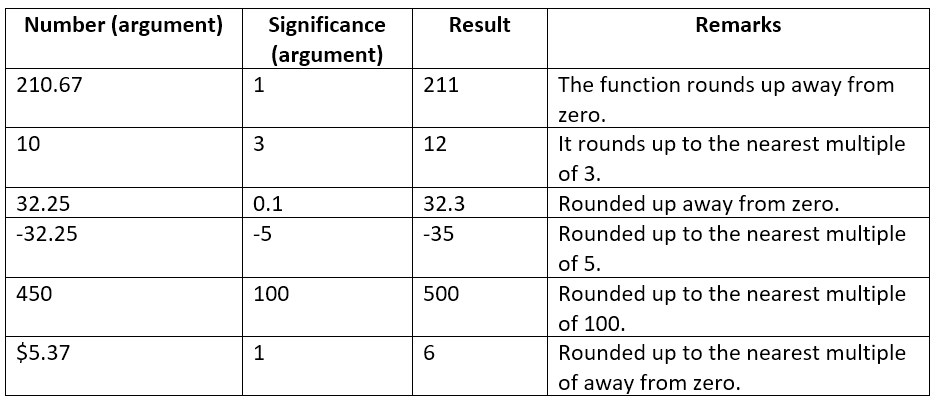
Let us take a set of positive integers as number arguments and positive numbers as significance, then apply the CEILING Excel function below. It will show the output in the result.

Example #2
In this example, we take a set of negative integers as number arguments and positive numbers as significance, then apply the CEILING Excel formula as shown in the table below. The output will be shown in the result as follows:

Example #3
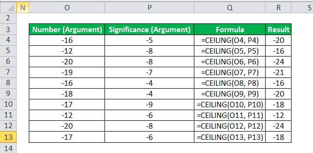
In this example, we take a set of negative integers as number arguments and negative numbers as significance, then apply the CEILING Excel formula to it.
Example #4
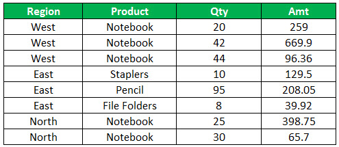
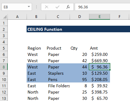
We can use the excel CEILING formula to highlight the rows in the group of given data, as shown in the below table. We will use the CEILING in Excel with ROW and ISEVEN functions.
Suppose we are given the data below:
Things to Remember
- #NUM! error:
- It may occur in MS Excel 2007 or earlier versions. For example, if we provide the significance argument with a different arithmetic sign from the given number argument, get #NUM! Error.
- It occurs if you are using MS Excel 2010/2013, then CEILING functions through #NUM! Error if the given number is positive and the supplied significance is negative.
- #DIV/0! Error occurs when the significance parameter is zero.
- #VALUE! Error occurs when any of the parameters is non-numeric.
- Excel CEILING function is the same as MROUND, but it always rounds up away from zero.
Recommended Articles
This article has been a guide to the CEILING function in Excel. Here we discuss the CEILING formula in Excel and how to use the CEILING function and Excel example, and downloadable Excel templates. You may also look at these useful functions in Excel: –
Источник
CEILING Function
Returns a number rounded up to a supplied number that is away from zero to the nearest multiple of a given number
What is the Excel CEILING Function?
The Excel CEILING function[1] is categorized under Math and Trigonometry functions. The function will return a number that is rounded up to a supplied number that is away from zero to the nearest multiple of a given number. MS Excel 2016 handles both positive and negative arguments.
The function is very useful in financial analysis as it helps in setting the price after currency conversion, discounts, etc. When preparing financial models, CEILING helps us round up the numbers as per the requirement. For example, if we provide =CEILING(10,5), the function will round off to the nearest 5 dollars.
Formula
=CEILING(number, significance)
The function uses the following arguments:
- Number (required argument) – This is the value that we wish to round off.
- Significance (required argument) – This is the multiple that we wish to round up to. It would use the same arithmetic sign (positive or negative) as per the provided number argument.
How to use the CEILING Function in Excel
To understand the uses of the CEILING function, let’s consider a few examples:
Example 1 – Excel Ceiling
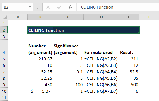
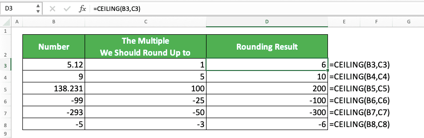
Let’s see the results from using the function when we provide the following data:
The formula used and results in Excel are shown in the screenshot below:
Example 2 – Using CEILING with other functions
We can use CEILING to highlight rows in a group of data. We will use a combination of ROW, CEILING, and ISEVEN functions. Suppose we are given the data below:
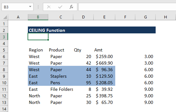
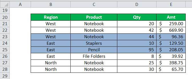
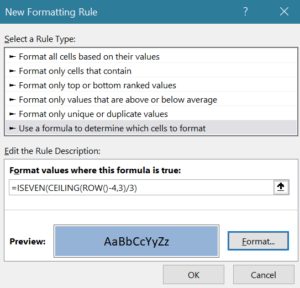
If we wish to highlight rows in groups of 3, we can use the formula =ISEVEN(CEILING(ROW()-4,3)/3) in conditional formatting.
We will get the result below:
In applying the function, remember to select the data before clicking on conditional formatting.
First, we “normalized” the row numbers to begin with 1, using the ROW function and an offset. Here 3 is n (the number of rows to group) and 4 is an offset to normalize the first row to 1 as the first row of data is in row 6. The CEILING function rounds incoming values up to a given multiple of n. Essentially, the CEILING function counts by a given multiple of n.
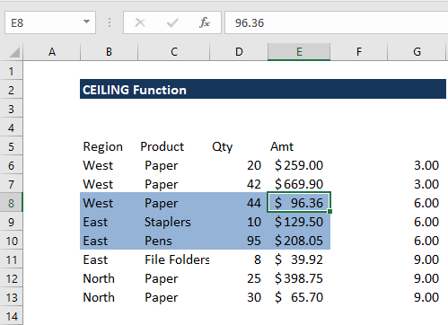
The count shown above in column G is then divided by n, that is in this case =3. Lastly, the ISEVEN function is used to force a TRUE result for all even row groups, which triggers the conditional formatting.
Notes about the Excel CEILING Function
- #NUM! error – Occurs when:
- If we are using MS Excel 2007 or earlier versions, provide the significance argument with a different arithmetic sign from the given number argument.
- If we are using MS Excel 2010 or 2013, if the given number is positive and the supplied significance is negative.
- #DIV/0! error – Occurs when the significance argument provided is 0.
- #VALUE! error – Occurs when any of the arguments is non-numeric.
- CEILING is like MROUND but it always rounds up away from zero.
Additional Resources
Thanks for reading CFI’s guide to important Excel functions! By taking the time to learn and master these functions, you’ll significantly speed up your financial analysis. To learn more, check out these additional CFI resources:
Источник
How to Use the CEILING Excel Formula: Functions, Examples and Writing Steps


In this tutorial, you will learn how to use the CEILING excel formula completely.
When working with numbers in excel, we sometimes need to round up a number to a certain multiple. If we use CEILING to do the rounding process, then we can get the result easily!
Want to master the method to use this CEILING formula in excel? Read this tutorial until its last part!
Disclaimer: This post may contain affiliate links from which we earn commission from qualifying purchases/actions at no additional cost for you. Learn more
Want to work faster and easier in Excel? Install and use Excel add-ins! Read this article to know the best Excel add-ins to use according to us!
What is the CEILING Formula in Excel?
CEILING Function in Excel
CEILING Result
Excel Version from Which We Can Use CEILING
The Way to Write It and Its Inputs
Here is the general writing form of a CEILING formula in excel.
And here is the explanation of the inputs we need to give in its formula writing.
- number_to_round = the number we want to round up to a certain multiple
- multiple = the multiple which we round up our number to
Example of Its Usage and Result
Here is the usage and result example of the CEILING formula in excel.
As you can see there, CEILING will always round up the number we input into it to the multiple we want. When we input negative numbers, CEILING will round our number away from zero.
Writing Steps
After discussing the writing form, inputs, and implementation example of CEILING, now let’s discuss its writing steps. As the inputs of this formula are quite simple, you should be able to understand the writing steps easily!
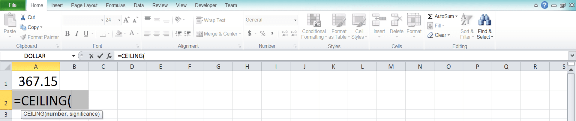
- Type an equal sign ( = ) in the cell where you want to put your CEILING result
Type CEILING (can be with large and small letters) and an open bracket sign after =
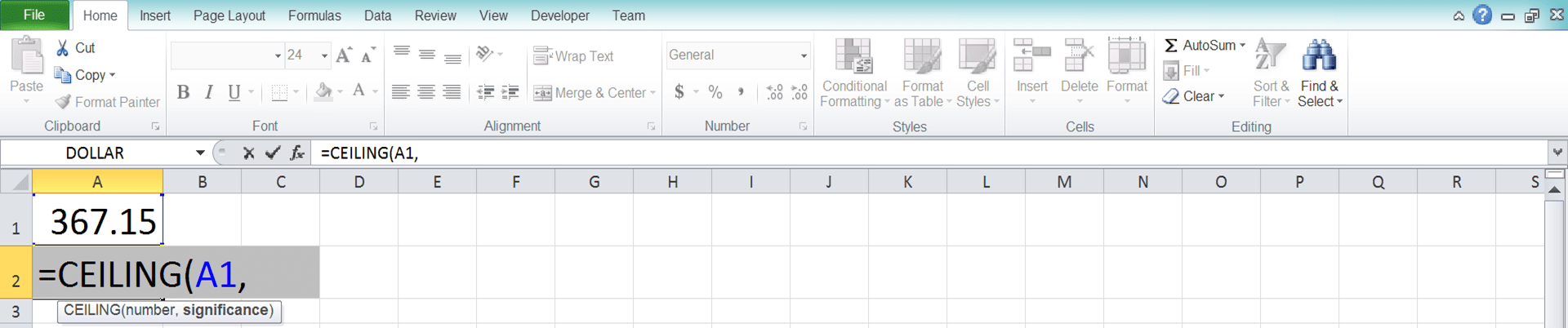
Input the number you want to round up to a certain multiple. Then, type a comma sign ( , )
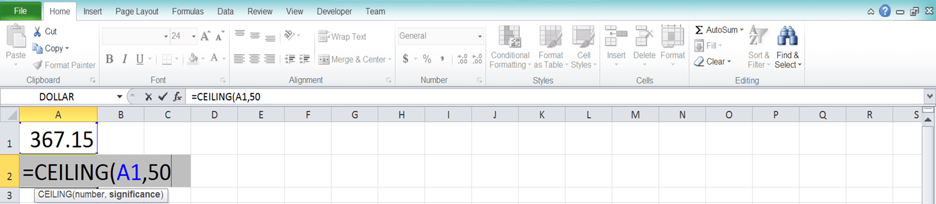
Input the multiple you want to round up your number to
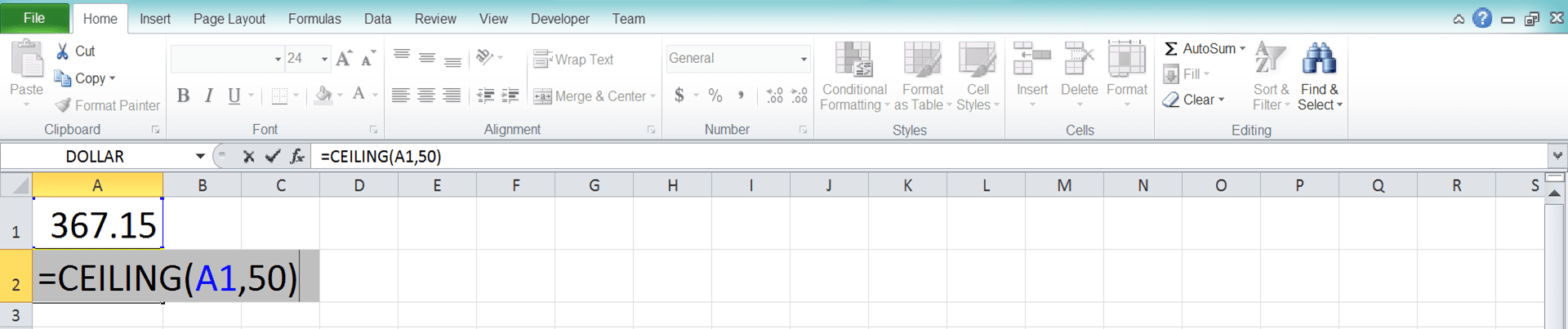
Type a close bracket sign
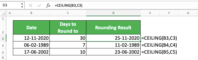
CEILING to Round Up Date
As the date is also a number data, we can use CEILING to round it up to a certain days multiple. Just input the date we want to round up and the days multiple we want to round our date to.
Here is the CEILING general writing form in excel to round up a date.
And here is its implementation example.
If you get a number from CEILING when you round up your date, just change its data type to date.
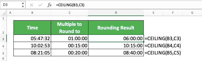
CEILING to Round Up Time
As time is a number data too, we can also round up time data using CEILING. Just input the time data you want to round up and the time multiple you want to round it to.
The time multiple you input to CEILING to round up time can be in hours, minutes, or seconds. Input it in the form of time data too so you can get your result correctly.
Here is the CEILING general writing form in excel to round up time.
And here is its implementation example.
Similar to date, if you get a number from CEILING instead of time, you should change the data type to time.
CEILING Alternative: CEILING.MATH
Since excel 2013, you can use CEILING.MATH as an alternative to CEILING.
If we look at the basic function, CEILING.MATH is the same as CEILING. They both help you to round up your number to a certain multiple.
There are two things, however, that become crucial differences when it comes to CEILING and CEILING.MATH.
- CEILING doesn’t have a default multiple input. That means you have to input a multiple to CEILING for the formula to run.
CEILING.MATH, meanwhile, has a default multiple input of 1. If you don’t give any multiple input to CEILING.MATH, it will round up your number to the multiple of 1
You can control your negative number rounding process with CEILING.MATH while you can’t do that with CEILING. If you use CEILING, you will round your negative number away from zero.
If you use CEILING.MATH, however, you can input whether you want to round it closer to or away from zero
Here is the general writing form of CEILING.MATH in excel.
You have one required input and two optional inputs in CEILING.MATH. For the required input, you must input the number you want to round as the first input of your CEILING.MATH.
For the negative number rounding mode, the default is you round your negative number closer to zero. If you input any non-zero value for it, you will round your negative number away from zero. If you input zero or don’t input anything, you will round it closer to zero.
For a better understanding of the formula, here is the implementation example of CEILING.MATH in excel.
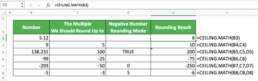
As you can see in the example, CEILING and CEILING.MATH round up positive numbers the same way. When we don’t input a multiple to CEILING.MATH, it will round our number up to the multiple of 1.
When we round a negative number, however, the default nature of CEILING.MATH is to round it closer to zero (the opposite of CEILING). We can input a non-zero value as its negative number rounding mode to round our negative number away from zero (TRUE is the same as 1 in excel, hence the rounding result for the third number in the example).
When you need the differences that CEILING.MATH gives, use it in your formula writing!
Exercise
After you have learned how to use the CEILING in excel, you can sharpen your understanding by doing the exercise below!
Download the exercise file from the following link and answer the questions. Download the answer key file to compare your answers with if you have done the exercise.
Link to the exercise file:
Download here
Questions
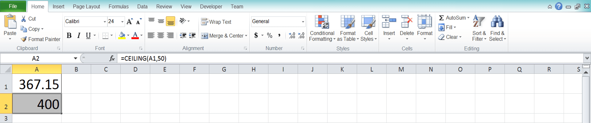
- What is the production quantity for the benchmark of the company’s factory if the standard batch is 10?
- What is the production quantity for the benchmark of the company’s factory if the standard batch is 50?
- What is the production quantity for the benchmark of the company’s factory if the standard batch is 1000?
Link to the answer key file:
Download here
Additional Note
If you round up a positive number to a negative multiple using CEILING, you will get a #NUM error.
Related tutorials you should learn from:
Источник
Функция ОКРВВЕРХ.МАТ округляет число с избытком до ближайшего целого или до ближайшего кратного указанному значению точности.
Описание функции ОКРВВЕРХ.МАТ
Округляет число с избытком до ближайшего целого или до ближайшего кратного указанному значению точности.
Синтаксис
=ОКРВВЕРХ(число; [точность]; [режим])Аргументы
числоточностьрежим
Обязательный. Должен быть меньше 9,99E+307 и больше -2,229E-308.
Необязательный. Кратное, до которого требуется округлить число.
Необязательный. Определяет, в какую сторону относительно нуля округляются отрицательные числа.
Замечания
- По умолчанию точность равна +1 для положительных чисел и -1 для отрицательных.
- По умолчанию положительные числа с дробной частью округляются до ближайшего целого числа. Например, 6,3 округляется до 7.
- По умолчанию отрицательные числа с дробной частью округляются (в сторону 0) до ближайшего целого числа. Например, -6,7 округляется до -6.
- Указывая аргументы «точность» и «режим», можно изменить направление округления отрицательных чисел. Например, округление -6,3 с точностью 1 и режимом 1 округляет в отрицательную сторону до -7. Существует много сочетаний значений точности и режима, которые по-разному влияют на округление отрицательных чисел.
- Аргумент «режим» не влияет на положительные числа.
- Аргумент «точность» округляет число с избытком до ближайшего целого числа, кратного указанной точности, кроме случаев, когда округляемое число ― целое. Например, с точностью 3 число округляется в сторону увеличения до следующего целого числа, кратного 3.
- Если при делении числа на точность 2 или больше возникает остаток, результат округляется в сторону увеличения.
Пример
Excel CEILING.MATH функция

Описание
Наблюдения и советы этой статьи мы подготовили на основании опыта команды CEILING.MATH функция округляет заданное число до ближайшего кратного значимости или до ближайшего целого числа.
Синтаксис и аргументы
Синтаксис формулы
=CEILING.MATH(number, [significance],[mode])
аргументы
- Number: Необходимые. Числовое значение, которое нужно округлить в большую сторону.
- Significance: Необязательный. Множитель, до которого нужно округлить число.
- Mode: Необязательный. При использовании функции CEILING.MATH решите округлять отрицательные числа в сторону или от нуля, по умолчанию — 0.
Возвращаемое значение
Наблюдения и советы этой статьи мы подготовили на основании опыта команды CEILING.MATH функция округляет число до ближайшего кратного.
Ноты:
1. Если значение опущено или значение по умолчанию, значение равно 1 для положительного числа и -1 для отрицательного числа. Например, 2 округляется до 2, -2 округляется до -2.
2. Если значение не указано или значение по умолчанию, положительные десятичные числа будут округлены до ближайшего целого числа. Например, округлите 1.23 до 2.
3. Если значение и режим опущены или заданы по умолчанию, отрицательные десятичные числа будут округлены до ближайшего целого числа, которое приближается к нулю. Например, округлите -1.23 до -1.
4. И число, и значимость отрицательны, результат округляется от нуля в меньшую сторону.
5. Если Mode не равен нулю, отрицательное число будет округлено до ближайшего кратного значимости, отличного от нуля, например, =CEILING.MATH(-12,5,1), от -12 до -15.
6. Если число является точным кратным значимости, изменений не происходит.
Использование и примеры
Вот несколько примеров, которые помогут вам понять, как использовать CEILING.MATH функция в Excel.
Положительное целое число
| Число | Значение | режим | Результат | Формула | Заметки |
| 8 | 8 | =CEILING.MATH(8) | Округлите 8 до ближайшего кратного 1 (по умолчанию) | ||
| 8 | 11 | 11 | =CEILING.MATH(8,11) | Округлите 8 до ближайшего числа, кратного 11 |
Положительное десятичное число
| Число | Значение | режим | Результат | Формула | Заметки |
| 1.23 | 2 | =CEILING.MATH(1.23) | Округлите 1.23 до ближайшего кратного 1 (по умолчанию) | ||
| 1.23 | 3 | 3 | =CEILING.MATH(1.23,3) | Округлите 1.23 до ближайшего числа, кратного 3 |
Положительное целое число
| Число | Значение | режим | Результат | Формула | Заметки |
| -10 | -10 | =CEILING.MATH(-10) | Округлить -10 до ближайшего кратного 1 (по умолчанию) и до нуля (по умолчанию) | ||
| -10 | 3 | -9 | =CEILING.MATH(-10,3) | Округлите -10 до ближайшего кратного 3, до нуля (по умолчанию). | |
| -10 | 3 | 1 | -12 | =CEILING.MATH(-10,3,1) | Округлить -10 до ближайшего кратного 3, от нуля |
Отрицательное десятичное число
| Число | Значение | режим | Результат | Формула | Заметки |
| -22.1 | -21 | =CEILING.MATH(-21.11) | Округлить -21.11 до ближайшего кратного 1 (по умолчанию) и до нуля (по умолчанию) | ||
| -22.1 | 10 | -20 | =CEILING.MATH(-21.11,10) | Округлите -21.11 до ближайшего кратного 10, до нуля (по умолчанию). | |
| -22.1 | 10 | 1 | -30 | =CEILING.MATH(-21.11,10,1) | Округлить -21.11 до ближайшего кратного 10, от нуля |
Скачать образец файла
 Нажмите, чтобы скачать CEILING.MATH файл образца функции
Относительные функции:
-
Excel CEILING Function
Наблюдения и советы этой статьи мы подготовили на основании опыта команды CEILING функция возвращает число, округленное до ближайшего кратного значимости. Например, = CEILING (10.12,0.2) возвращает 10.2, округляя 10.12 до ближайшего кратного 0.2. -
Excel CEILING.PRECISE Функция
Наблюдения и советы этой статьи мы подготовили на основании опыта команды CEILING.PRECISE Функция возвращает число, округленное до ближайшего кратного или ближайшего целого числа, игнорируя знак числа, округляет все числа в большую сторону.
Относительные статьи:
-
Округление числа до ближайшего числа 5,10, 50 или 100 в Excel
В этой статье представлены некоторые простые формулы для округления чисел до ближайшего определенного числа, а также представлены формулы для округления чисел до следующего или последнего ближайшего числа.
Лучшие инструменты для работы в офисе
Kutools for Excel — Помогает вам выделиться из толпы
Хотите быстро и качественно выполнять свою повседневную работу? Kutools for Excel предлагает 300 мощных расширенных функций (объединение книг, суммирование по цвету, разделение содержимого ячеек, преобразование даты и т. д.) и экономит для вас 80 % времени.
- Разработан для 1500 рабочих сценариев, помогает решить 80% проблем с Excel.
- Уменьшите количество нажатий на клавиатуру и мышь каждый день, избавьтесь от усталости глаз и рук.
- Станьте экспертом по Excel за 3 минуты. Больше не нужно запоминать какие-либо болезненные формулы и коды VBA.
- 30-дневная неограниченная бесплатная пробная версия. 60-дневная гарантия возврата денег. Бесплатное обновление и поддержка 2 года.
")
Вкладка Office — включение чтения и редактирования с вкладками в Microsoft Office (включая Excel)
- Одна секунда для переключения между десятками открытых документов!
- Уменьшите количество щелчков мышью на сотни каждый день, попрощайтесь с рукой мыши.
- Повышает вашу продуктивность на 50% при просмотре и редактировании нескольких документов.
- Добавляет эффективные вкладки в Office (включая Excel), точно так же, как Chrome, Firefox и новый Internet Explorer.
")
Комментарии (0)
Оценок пока нет. Оцените первым!
Home > Microsoft Excel > How to Use the CEILING Function in Excel? A Step-by-Step Guide
(Note: This guide on how to use the CEILING function in Excel is suitable for all Excel versions including Office 365)
Functions are an integral part of operations in Excel. Using functions, you can accomplish various tasks with ease. Excel contains a variety of functions that can be tailored based on the user’s needs and get the desired output.
In some cases, you might want to find the rounded-up value of a particular data which is usually greater than the number. To get the resultant value, you can use the CEILING function in Excel.
In this article, I will tell you how to use the CEILING function in Excel.
You’ll Learn:
- What Is the CEILING Function in Excel?
- Syntax
- How to Use the CEILING Function in Excel?
- How Does the CEILING Function Work?
- Other Use Cases
- Points to Remember

Related Reads:
How to Use FLOOR Function in Excel? 2 Easy Ways
How to Calculate IRR in Excel? 3 Important Functions
How to Use Excel MATCH Function? 3 Use Cases
What Is the CEILING Function in Excel?
The Excel CEILING function is a part of the Math & Trigonometry set of functions and it can be found under the name CEILING.MATH.
The CEILING function is similar to the roundup function. This function returns a rounded number greater than the nearest multiple of the given significant digit.
Syntax
=CEILING(number, significant_value)
Where
number argument refers to the value to be rounded. It is a mandatory field and it can either take up a constant number value or a cell value which refers to the constant value.
significant_value is also a mandatory field. This field denotes the multiples to which the numerical values should be rounded.
How to Use the CEILING Function in Excel?
You can use the CEILING function in Excel in two ways. It can be done by manually entering the formula into the cell or by choosing it from the Formulas tab.
By Entering the Formula
The first method is a pretty common way of using formulas. In this method, you can directly enter the formula into the cell and pass the arguments.
- To use the CEILING function in Excel, first, select a destination cell.
- In the destination cell, enter the formula =CEILING. Once you start typing the formula, the formula suggestions start showing up. Press the Tab key to select the formula.
- Choose CEILING.MATH function either by double-clicking on it or by pressing the Tab key.

- Now, let’s pass on the arguments.
- You can pass the arguments as a constant value or a variable that points out the value in a cell. In this case, let us pass the number argument as A4 and the significance argument as B4. the cells A4 and B4 contain the values 13 and 2 respectively.
- Now, press Enter.

This gives the ceiling value of the values based on the significant digits.
By Selecting From the Formulas List
Another way to use the CEILING function is by selecting it from the Formulas menu. This method greatly helps you find the correct formula when you’re unsure of the particular formula.
- To use this method, first, choose a destination cell.
- Then, navigate to the Formulas main menu ribbon, and under the Function Library, click on the dropdown from Math & Trig.
- Scroll down and select CEILING.MATH function.

- This opens the Functions Arguments dialog box.
- In the Function Arguments dialog box, you can either pass the arguments by entering the constant values directly or by selecting the cell that contains the value.

- Once you have populated the arguments, press OK.
- This gives you the resultant value in the destination cell.
Suggested Reads:
How to Use CONVERT Function in Excel? A Step-by-Step Guide
How to Use the Excel TREND Function? A Step-by-Step Guide
How to Use SUMPRODUCT Function in Excel? 5 Easy Examples
How Does the CEILING Function Work?
Above, we saw how to use the CEILING function either by entering the formula or by choosing it from the list of formulas. But, how does the function work and how does it give the resultant value?
Let us see how.
The CEILING function works by rounding up the numerical value to the corresponding significant digits.
Let us consider the above example, where the number value is 13 and its significance is 2.
The multiples of 2 are 2, 4, 6, 8,10, 12, 14, 16, and so on. Here, the value 13 lies between 14 and 16 (which are multiples of 2). Since the CEILING function always rounds up the value, it chooses the largest value 14, and returns the value.
Other Use Cases

- Let’s take the number argument as the decimal value 6.7 and the significance as 2. Upon applying the CEILING function, the value 6.7 is rounded up to the value 8, as 8 is the next greatest value which is a multiple of 2.
- If both the number argument and significance are negative, then the CEILING function in Excel returns the number away from zero. Consider the number value -2.6 and the significance is -3, the CEILING function returns the value -3. This is because -2.6 lies between -3 and 0, with -3 being the nearest multiple.
- In the case where the number argument is a negative value and significance is a positive value, the CEILING function returns the nearby greater value close to 0. Consider the example, where the number is -3.4 and the significance is 2, then the CEILING function returns the value -2.
- The CEILING function returns an error when the number value is positive and the significance is negative. For example, if the number value is 4.5 and the significance is -2, the CEILING function returns #NUM! Error.
- When the number value is 2.38 and the significance is 0.1, the ceiling value becomes 2.4 as it is the nearest greater multiple 0f 0.1.
- Likewise, consider the number value 2.3845 with a significant value of 0.01. The CEILING function returns the value 2.39.
Points to Remember
- The CEILING function always returns a #VALUE! error if the number or the significance argument is a non-numerical value.
- When the argument is positive and the significant value is negative, the CEILING function returns a #NUM! Error.
- The CEILING function does not round the value when the number value is an exact multiple of the digit.
- The CEILING value is rounded up towards zero if the number argument is positive.
- The greater the significance, the greater will be the difference between the resultant ceiling values and the number value.
Also Read:
How to Use the ROUND Function in Excel?
Battle of the Excel Lookup Functions: VLOOKUP vs INDEX/MATCH vs XLOOKUP
How to Use the Excel IFS Function? – 2 Easy Examples
Frequently Asked Questions
What is the formula to calculate the ceiling value in Excel?
To use the CEILING function, choose a destination cell and enter the formula =CEILING(number,significance). Here, the number value represents the number value to be rounded and significance represents the multiples to which the numerical values should be rounded.
How to find the CEILING function in the Formulas tab?
The Excel CEILING function can be found under the Math and Trigonometry category in the Formulas main menu ribbon under the name =CEILING.MATH.
Final Thoughts
Rounding up a number to the multiples of the significant digits using the CEILING function can be used in a variety of places. In this article, we saw how to use the CEILING function in Excel. We also saw 2 different ways to use the function along with its use cases.
Please visit our free resources center for more high-quality guides on Excel and other Microsoft Suite applications.
Ready to dive deep into Excel? Click here for advanced Excel courses with in-depth training modules.
Simon Sez IT has been teaching Excel and other business software for over ten years. For a low, monthly fee you can get access to 150+ IT training courses.

Simon Calder

Chris “Simon” Calder was working as a Project Manager in IT for one of Los Angeles’ most prestigious cultural institutions, LACMA.He taught himself to use Microsoft Project from a giant textbook and hated every moment of it. Online learning was in its infancy then, but he spotted an opportunity and made an online MS Project course — the rest, as they say, is history!