
This article explains in simple terms how to use INDEX and MATCH together to perform lookups. It takes a step-by-step approach, first explaining INDEX, then MATCH, then showing you how to combine the two functions together to create a dynamic two-way lookup. There are more advanced examples further down the page.
INDEX function | MATCH function | INDEX and MATCH | 2-way lookup | Left lookup | Case-sensitive | Closest match | Multiple criteria | More examples
The INDEX Function
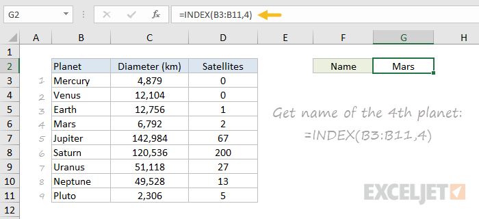
The INDEX function in Excel is fantastically flexible and powerful, and you’ll find it in a huge number of Excel formulas, especially advanced formulas. But what does INDEX actually do? In a nutshell, INDEX retrieves the value at a given location in a range. For example, let’s say you have a table of planets in our solar system (see below), and you want to get the name of the 4th planet, Mars, with a formula. You can use INDEX like this:
=INDEX(B3:B11,4)

INDEX returns the value in the 4th row of the range.
Video: How to look things up with INDEX
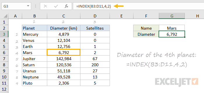
What if you want to get the diameter of Mars with INDEX? In that case, we can supply both a row number and a column number, and provide a larger range. The INDEX formula below uses the full range of data in B3:D11, with a row number of 4 and column number of 2:
=INDEX(B3:D11,4,2)

INDEX retrieves the value at row 4, column 2.
To summarize, INDEX gets a value at a given location in a range of cells based on numeric position. When the range is one-dimensional, you only need to supply a row number. When the range is two-dimensional, you’ll need to supply both the row and column number.
At this point, you may be thinking «So what? How often do you actually know the position of something in a spreadsheet?»
Exactly right. We need a way to locate the position of things we’re looking for.
Enter the MATCH function.
The MATCH function
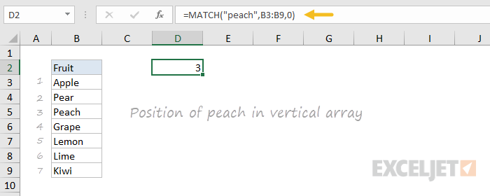
The MATCH function is designed for one purpose: find the position of an item in a range. For example, we can use MATCH to get the position of the word «peach» in this list of fruits like this:
=MATCH("peach",B3:B9,0)

MATCH returns 3, since «Peach» is the 3rd item. MATCH is not case-sensitive.
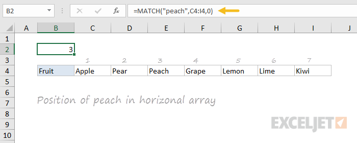
MATCH doesn’t care if a range is horizontal or vertical, as you can see below:
=MATCH("peach",C4:I4,0)

Same result with a horizontal range, MATCH returns 3.
Video: How to use MATCH for exact matches
Important: The last argument in the MATCH function is match_type. Match_type is important and controls whether matching is exact or approximate. In many cases you will want to use zero (0) to force exact match behavior. Match_type defaults to 1, which means approximate match, so it’s important to provide a value. See the MATCH page for more details.
INDEX and MATCH together
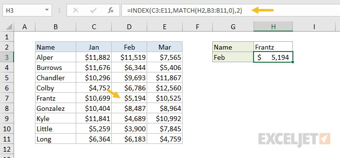
Now that we’ve covered the basics of INDEX and MATCH, how do we combine the two functions in a single formula? Consider the data below, a table showing a list of salespeople and monthly sales numbers for three months: January, February, and March.

Let’s say we want to write a formula that returns the sales number for February for a given salesperson. From the discussion above, we know we can give INDEX a row and column number to retrieve a value. For example, to return the February sales number for Frantz, we provide the range C3:E11 with a row 5 and column 2:
=INDEX(C3:E11,5,2) // returns $5194
But we obviously don’t want to hardcode numbers. Instead, we want a dynamic lookup.
How will we do that? The MATCH function of course. MATCH will work perfectly for finding the positions we need. Working one step at a time, let’s leave the column hardcoded as 2 and make the row number dynamic. Here’s the revised formula, with the MATCH function nested inside INDEX in place of 5:
=INDEX(C3:E11,MATCH("Frantz",B3:B11,0),2)
Taking things one step further, we’ll use the value from H2 in MATCH:
=INDEX(C3:E11,MATCH(H2,B3:B11,0),2)

MATCH finds «Frantz» and returns 5 to INDEX for row.
To summarize:
- INDEX needs numeric positions.
- MATCH finds those positions.
- MATCH is nested inside INDEX.
Let’s now tackle the column number.
Two-way lookup with INDEX and MATCH
Above, we used the MATCH function to find the row number dynamically, but hardcoded the column number. How can we make the formula fully dynamic, so we can return sales for any given salesperson in any given month? The trick is to use MATCH twice – once to get a row position, and once to get a column position.
From the examples above, we know MATCH works fine with both horizontal and vertical arrays. That means we can easily find the position of a given month with MATCH. For example, this formula returns the position of March, which is 3:
=MATCH("Mar",C2:E2,0) // returns 3
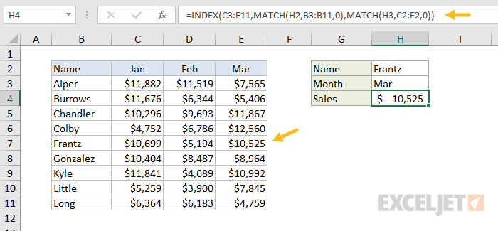
But of course we don’t want to hardcode any values, so let’s update the worksheet to allow the input of a month name, and use MATCH to find the column number we need. The screen below shows the result:

A fully dynamic, two-way lookup with INDEX and MATCH.
=INDEX(C3:E11,MATCH(H2,B3:B11,0),MATCH(H3,C2:E2,0))
The first MATCH formula returns 5 to INDEX as the row number, the second MATCH formula returns 3 to INDEX as the column number. Once MATCH runs, the formula simplifies to:
=INDEX(C3:E11,5,3)
and INDEX correctly returns $10,525, the sales number for Frantz in March.
Note: you could use Data Validation to create dropdown menus to select salesperson and month.
Video: How to do a two-way lookup with INDEX and MATCH
Video: How to debug a formula with F9 (to see MATCH return values)
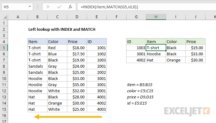
Left lookup
One of the key advantages of INDEX and MATCH over the VLOOKUP function is the ability to perform a «left lookup». Simply put, this just means a lookup where the ID column is to the right of the values you want to retrieve, as seen in the example below:

Read a detailed explanation here.
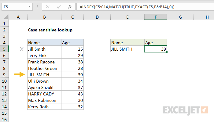
Case-sensitive lookup
By itself, the MATCH function is not case-sensitive. However, you use the EXACT function with INDEX and MATCH to perform a lookup that respects upper and lower case, as shown below:

Read a detailed explanation here.
Note: this is an array formula and must be entered with control + shift + enter, except in Excel 365.
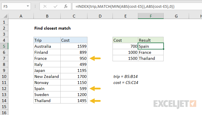
Closest match
Another example that shows off the flexibility of INDEX and MATCH is the problem of finding the closest match. In the example below, we use the MIN function together with the ABS function to create a lookup value and a lookup array inside the MATCH function. Essentially, we use MATCH to find the smallest difference. Then we use INDEX to retrieve the associated trip from column B.

Read a detailed explanation here.
Note: this is an array formula and must be entered with control + shift + enter, except in Excel 365.
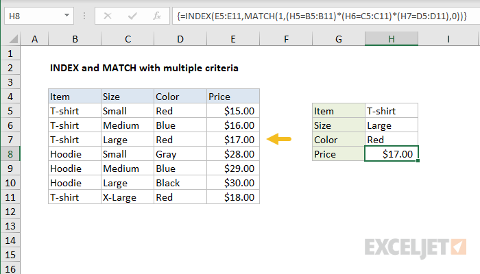
Multiple criteria lookup
One of the trickiest problems in Excel is a lookup based on multiple criteria. In other words, a lookup that matches on more than one column at the same time. In the example below, we are using INDEX and MATCH and boolean logic to match on 3 columns: Item, Color, and Size:

Read a detailed explanation here. You can use this same approach with XLOOKUP.
Note: this is an array formula and must be entered with control + shift + enter, except in Excel 365.
More examples of INDEX + MATCH
Here are some more basic examples of INDEX and MATCH in action, each with a detailed explanation:
- Basic INDEX and MATCH exact (features Toy Story)
- Basic INDEX and MATCH approximate (grades)
- Two-way lookup with INDEX and MATCH (approximate match)
Tip: Try using the new XLOOKUP and XMATCH functions, improved versions of the functions described in this article. These new functions work in any direction and return exact matches by default, making them easier and more convenient to use than their predecessors.
Suppose that you have a list of office location numbers, and you need to know which employees are in each office. The spreadsheet is huge, so you might think it is challenging task. It’s actually quite easy to do with a lookup function.
The VLOOKUP and HLOOKUP functions, together with INDEX and MATCH, are some of the most useful functions in Excel.
Note: The Lookup Wizard feature is no longer available in Excel.
Here’s an example of how to use VLOOKUP.
=VLOOKUP(B2,C2:E7,3,TRUE)
In this example, B2 is the first argument—an element of data that the function needs to work. For VLOOKUP, this first argument is the value that you want to find. This argument can be a cell reference, or a fixed value such as «smith» or 21,000. The second argument is the range of cells, C2-:E7, in which to search for the value you want to find. The third argument is the column in that range of cells that contains the value that you seek.
The fourth argument is optional. Enter either TRUE or FALSE. If you enter TRUE, or leave the argument blank, the function returns an approximate match of the value you specify in the first argument. If you enter FALSE, the function will match the value provide by the first argument. In other words, leaving the fourth argument blank—or entering TRUE—gives you more flexibility.
This example shows you how the function works. When you enter a value in cell B2 (the first argument), VLOOKUP searches the cells in the range C2:E7 (2nd argument) and returns the closest approximate match from the third column in the range, column E (3rd argument).
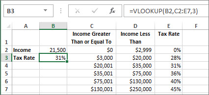
The fourth argument is empty, so the function returns an approximate match. If it didn’t, you’d have to enter one of the values in columns C or D to get a result at all.
When you’re comfortable with VLOOKUP, the HLOOKUP function is equally easy to use. You enter the same arguments, but it searches in rows instead of columns.
Using INDEX and MATCH instead of VLOOKUP
There are certain limitations with using VLOOKUP—the VLOOKUP function can only look up a value from left to right. This means that the column containing the value you look up should always be located to the left of the column containing the return value. Now if your spreadsheet isn’t built this way, then do not use VLOOKUP. Use the combination of INDEX and MATCH functions instead.
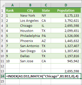
This example shows a small list where the value we want to search on, Chicago, isn’t in the leftmost column. So, we can’t use VLOOKUP. Instead, we’ll use the MATCH function to find Chicago in the range B1:B11. It’s found in row 4. Then, INDEX uses that value as the lookup argument, and finds the population for Chicago in the 4th column (column D). The formula used is shown in cell A14.
For more examples of using INDEX and MATCH instead of VLOOKUP, see the article https://www.mrexcel.com/excel-tips/excel-vlookup-index-match/ by Bill Jelen, Microsoft MVP.
Give it a try
If you want to experiment with lookup functions before you try them out with your own data, here’s some sample data.
VLOOKUP Example at work
Copy the following data into a blank spreadsheet.
Tip: Before you paste the data into Excel, set the column widths for columns A through C to 250 pixels, and click Wrap Text (Home tab, Alignment group).
|
Density |
Viscosity |
Temperature |
|
0.457 |
3.55 |
500 |
|
0.525 |
3.25 |
400 |
|
0.606 |
2.93 |
300 |
|
0.675 |
2.75 |
250 |
|
0.746 |
2.57 |
200 |
|
0.835 |
2.38 |
150 |
|
0.946 |
2.17 |
100 |
|
1.09 |
1.95 |
50 |
|
1.29 |
1.71 |
0 |
|
Formula |
Description |
Result |
|
=VLOOKUP(1,A2:C10,2) |
Using an approximate match, searches for the value 1 in column A, finds the largest value less than or equal to 1 in column A which is 0.946, and then returns the value from column B in the same row. |
2.17 |
|
=VLOOKUP(1,A2:C10,3,TRUE) |
Using an approximate match, searches for the value 1 in column A, finds the largest value less than or equal to 1 in column A, which is 0.946, and then returns the value from column C in the same row. |
100 |
|
=VLOOKUP(0.7,A2:C10,3,FALSE) |
Using an exact match, searches for the value 0.7 in column A. Because there is no exact match in column A, an error is returned. |
#N/A |
|
=VLOOKUP(0.1,A2:C10,2,TRUE) |
Using an approximate match, searches for the value 0.1 in column A. Because 0.1 is less than the smallest value in column A, an error is returned. |
#N/A |
|
=VLOOKUP(2,A2:C10,2,TRUE) |
Using an approximate match, searches for the value 2 in column A, finds the largest value less than or equal to 2 in column A, which is 1.29, and then returns the value from column B in the same row. |
1.71 |
HLOOKUP Example
Copy all the cells in this table and paste it into cell A1 on a blank worksheet in Excel.
Tip: Before you paste the data into Excel, set the column widths for columns A through C to 250 pixels, and click Wrap Text (Home tab, Alignment group).
|
Axles |
Bearings |
Bolts |
|
4 |
4 |
9 |
|
5 |
7 |
10 |
|
6 |
8 |
11 |
|
Formula |
Description |
Result |
|
=HLOOKUP(«Axles», A1:C4, 2, TRUE) |
Looks up «Axles» in row 1, and returns the value from row 2 that’s in the same column (column A). |
4 |
|
=HLOOKUP(«Bearings», A1:C4, 3, FALSE) |
Looks up «Bearings» in row 1, and returns the value from row 3 that’s in the same column (column B). |
7 |
|
=HLOOKUP(«B», A1:C4, 3, TRUE) |
Looks up «B» in row 1, and returns the value from row 3 that’s in the same column. Because an exact match for «B» is not found, the largest value in row 1 that is less than «B» is used: «Axles,» in column A. |
5 |
|
=HLOOKUP(«Bolts», A1:C4, 4) |
Looks up «Bolts» in row 1, and returns the value from row 4 that’s in the same column (column C). |
11 |
|
=HLOOKUP(3, {1,2,3;»a»,»b»,»c»;»d»,»e»,»f»}, 2, TRUE) |
Looks up the number 3 in the three-row array constant, and returns the value from row 2 in the same (in this case, third) column. There are three rows of values in the array constant, each row separated by a semicolon (;). Because «c» is found in row 2 and in the same column as 3, «c» is returned. |
c |
INDEX and MATCH Examples
This last example employs the INDEX and MATCH functions together to return the earliest invoice number and its corresponding date for each of five cities. Because the date is returned as a number, we use the TEXT function to format it as a date. The INDEX function actually uses the result of the MATCH function as its argument. The combination of the INDEX and MATCH functions are used twice in each formula – first, to return the invoice number, and then to return the date.
Copy all the cells in this table and paste it into cell A1 on a blank worksheet in Excel.
Tip: Before you paste the data into Excel, set the column widths for columns A through D to 250 pixels, and click Wrap Text (Home tab, Alignment group).
|
Invoice |
City |
Invoice Date |
Earliest invoice by city, with date |
|
3115 |
Atlanta |
4/7/12 |
=»Atlanta = «&INDEX($A$2:$C$33,MATCH(«Atlanta»,$B$2:$B$33,0),1)& «, Invoice date: » & TEXT(INDEX($A$2:$C$33,MATCH(«Atlanta»,$B$2:$B$33,0),3),»m/d/yy») |
|
3137 |
Atlanta |
4/9/12 |
=»Austin = «&INDEX($A$2:$C$33,MATCH(«Austin»,$B$2:$B$33,0),1)& «, Invoice date: » & TEXT(INDEX($A$2:$C$33,MATCH(«Austin»,$B$2:$B$33,0),3),»m/d/yy») |
|
3154 |
Atlanta |
4/11/12 |
=»Dallas = «&INDEX($A$2:$C$33,MATCH(«Dallas»,$B$2:$B$33,0),1)& «, Invoice date: » & TEXT(INDEX($A$2:$C$33,MATCH(«Dallas»,$B$2:$B$33,0),3),»m/d/yy») |
|
3191 |
Atlanta |
4/21/12 |
=»New Orleans = «&INDEX($A$2:$C$33,MATCH(«New Orleans»,$B$2:$B$33,0),1)& «, Invoice date: » & TEXT(INDEX($A$2:$C$33,MATCH(«New Orleans»,$B$2:$B$33,0),3),»m/d/yy») |
|
3293 |
Atlanta |
4/25/12 |
=»Tampa = «&INDEX($A$2:$C$33,MATCH(«Tampa»,$B$2:$B$33,0),1)& «, Invoice date: » & TEXT(INDEX($A$2:$C$33,MATCH(«Tampa»,$B$2:$B$33,0),3),»m/d/yy») |
|
3331 |
Atlanta |
4/27/12 |
|
|
3350 |
Atlanta |
4/28/12 |
|
|
3390 |
Atlanta |
5/1/12 |
|
|
3441 |
Atlanta |
5/2/12 |
|
|
3517 |
Atlanta |
5/8/12 |
|
|
3124 |
Austin |
4/9/12 |
|
|
3155 |
Austin |
4/11/12 |
|
|
3177 |
Austin |
4/19/12 |
|
|
3357 |
Austin |
4/28/12 |
|
|
3492 |
Austin |
5/6/12 |
|
|
3316 |
Dallas |
4/25/12 |
|
|
3346 |
Dallas |
4/28/12 |
|
|
3372 |
Dallas |
5/1/12 |
|
|
3414 |
Dallas |
5/1/12 |
|
|
3451 |
Dallas |
5/2/12 |
|
|
3467 |
Dallas |
5/2/12 |
|
|
3474 |
Dallas |
5/4/12 |
|
|
3490 |
Dallas |
5/5/12 |
|
|
3503 |
Dallas |
5/8/12 |
|
|
3151 |
New Orleans |
4/9/12 |
|
|
3438 |
New Orleans |
5/2/12 |
|
|
3471 |
New Orleans |
5/4/12 |
|
|
3160 |
Tampa |
4/18/12 |
|
|
3328 |
Tampa |
4/26/12 |
|
|
3368 |
Tampa |
4/29/12 |
|
|
3420 |
Tampa |
5/1/12 |
|
|
3501 |
Tampa |
5/6/12 |
Содержание
- Функции MS Excel ИНДЕКС (INDEX) и ПОИСКПОЗ (MATCH) – более гибкая альтернатива ВПР
- Look up values with VLOOKUP, INDEX, or MATCH
- Using INDEX and MATCH instead of VLOOKUP
- Give it a try
- VLOOKUP Example at work
- How to use INDEX and MATCH
- Summary
- The INDEX Function
- The MATCH function
- INDEX and MATCH together
- Two-way lookup with INDEX and MATCH
- Left lookup
- Case-sensitive lookup
- Closest match
- Multiple criteria lookup
- More examples of INDEX + MATCH
Функции MS Excel ИНДЕКС (INDEX) и ПОИСКПОЗ (MATCH) – более гибкая альтернатива ВПР
Многие пользователи знают и применяют формулу ВПР. Известно также, что ВПР имеет ряд особенностей и ограничений, которые несложно обойти. Однако есть нюанс, который значительно ограничивает возможности функции ВПР.
ВПР требует, чтобы в диапазоне с искомыми данными столбец критериев всегда был первым слева. Это обстоятельство, конечно, является ограничением ВПР. Как же быть, если искомые данные находятся левее столбца с критерием? Можно, конечно, расположить столбцы в нужном порядке, что в целом, является неплохим выходом из ситуации. Но бывает так, что сделать этого нельзя, или трудно. К примеру, вы работаете в чужом документе или регулярно получаете новый отчет. В общем, нужно решение, не зависящее от расположения столбцов. Такое решение существует.
Нужно воспользоваться комбинацией из двух функций: ИНДЕКС и ПОИСКПОЗ. Формула работает следующим образом. ИНДЕКС отсчитывает необходимое количество ячеек вниз в диапазоне искомых значений. Количество отсчитываемых ячеек определяется по столбцу критериев функцией ПОИСКПОЗ. Работу комбинации этих функций удобно рассмотреть с середины, где вначале находится номер ячейки с подходящим критерием, а затем этот номер подставляется в ИНДЕКС.

Таким образом, чтобы подтянуть значение цены, соответствующее первому коду (книге), нужно прописать такую формулу.

Следует обратить внимание на корректность ссылок, чтобы при копировании формулы ничего не «съехало». Протягиваем формулу вниз. Если в таблице, откуда подтягиваются данные, нет искомого критерия, то функция выдает ошибку #Н/Д.

Довольно стандартная ситуация, с которой успешно справляется функция ЕСЛИОШИБКА. Она перехватывает ошибки и вместо них выдает что-либо другое, например, нули.
Конструкция формулы будет следующая:

Вот, собственно, и все.
Таким образом, комбинация функций ИНДЕКС и ПОИСКПОЗ является полной заменой ВПР и обладает дополнительным преимуществом: умеет находить данные слева от столбца с критерием. Кроме того, сами столбцы можно двигать как угодно, лишь бы ссылка не съехала, чего нельзя проделать с ВПР, т.к. количество столбцов там указывается конкретным числом. Посему комбинация ИНДЕКС и ПОИСКПОЗ более универсальна, чем ВПР.
Ниже видеоурок по работе функций ИНДЕКС и ПОИСКПОЗ.
Источник
Look up values with VLOOKUP, INDEX, or MATCH
Tip: Try using the new XLOOKUP and XMATCH functions, improved versions of the functions described in this article. These new functions work in any direction and return exact matches by default, making them easier and more convenient to use than their predecessors.
Suppose that you have a list of office location numbers, and you need to know which employees are in each office. The spreadsheet is huge, so you might think it is challenging task. It’s actually quite easy to do with a lookup function.
The VLOOKUP and HLOOKUP functions, together with INDEX and MATCH, are some of the most useful functions in Excel.
Note: The Lookup Wizard feature is no longer available in Excel.
Here’s an example of how to use VLOOKUP.
In this example, B2 is the first argument—an element of data that the function needs to work. For VLOOKUP, this first argument is the value that you want to find. This argument can be a cell reference, or a fixed value such as «smith» or 21,000. The second argument is the range of cells, C2-:E7, in which to search for the value you want to find. The third argument is the column in that range of cells that contains the value that you seek.
The fourth argument is optional. Enter either TRUE or FALSE. If you enter TRUE, or leave the argument blank, the function returns an approximate match of the value you specify in the first argument. If you enter FALSE, the function will match the value provide by the first argument. In other words, leaving the fourth argument blank—or entering TRUE—gives you more flexibility.
This example shows you how the function works. When you enter a value in cell B2 (the first argument), VLOOKUP searches the cells in the range C2:E7 (2nd argument) and returns the closest approximate match from the third column in the range, column E (3rd argument).
The fourth argument is empty, so the function returns an approximate match. If it didn’t, you’d have to enter one of the values in columns C or D to get a result at all.
When you’re comfortable with VLOOKUP, the HLOOKUP function is equally easy to use. You enter the same arguments, but it searches in rows instead of columns.
Using INDEX and MATCH instead of VLOOKUP
There are certain limitations with using VLOOKUP—the VLOOKUP function can only look up a value from left to right. This means that the column containing the value you look up should always be located to the left of the column containing the return value. Now if your spreadsheet isn’t built this way, then do not use VLOOKUP. Use the combination of INDEX and MATCH functions instead.
This example shows a small list where the value we want to search on, Chicago, isn’t in the leftmost column. So, we can’t use VLOOKUP. Instead, we’ll use the MATCH function to find Chicago in the range B1:B11. It’s found in row 4. Then, INDEX uses that value as the lookup argument, and finds the population for Chicago in the 4th column (column D). The formula used is shown in cell A14.
For more examples of using INDEX and MATCH instead of VLOOKUP, see the article https://www.mrexcel.com/excel-tips/excel-vlookup-index-match/ by Bill Jelen, Microsoft MVP.
Give it a try
If you want to experiment with lookup functions before you try them out with your own data, here’s some sample data.
VLOOKUP Example at work
Copy the following data into a blank spreadsheet.
Tip: Before you paste the data into Excel, set the column widths for columns A through C to 250 pixels, and click Wrap Text ( Home tab, Alignment group).
Источник
How to use INDEX and MATCH

Summary
INDEX and MATCH is the most popular tool in Excel for performing more advanced lookups. This is because INDEX and MATCH are incredibly flexible – you can do horizontal and vertical lookups, 2-way lookups, left lookups, case-sensitive lookups, and even lookups based on multiple criteria. If you want to improve your Excel skills, INDEX and MATCH should be on your list. See below for many examples.
This article explains in simple terms how to use INDEX and MATCH together to perform lookups. It takes a step-by-step approach, first explaining INDEX, then MATCH, then showing you how to combine the two functions together to create a dynamic two-way lookup. There are more advanced examples further down the page.
The INDEX Function
The INDEX function in Excel is fantastically flexible and powerful, and you’ll find it in a huge number of Excel formulas, especially advanced formulas. But what does INDEX actually do? In a nutshell, INDEX retrieves the value at a given location in a range. For example, let’s say you have a table of planets in our solar system (see below), and you want to get the name of the 4th planet, Mars, with a formula. You can use INDEX like this:
INDEX returns the value in the 4th row of the range.
What if you want to get the diameter of Mars with INDEX? In that case, we can supply both a row number and a column number, and provide a larger range. The INDEX formula below uses the full range of data in B3:D11, with a row number of 4 and column number of 2:
INDEX retrieves the value at row 4, column 2.
To summarize, INDEX gets a value at a given location in a range of cells based on numeric position. When the range is one-dimensional, you only need to supply a row number. When the range is two-dimensional, you’ll need to supply both the row and column number.
At this point, you may be thinking «So what? How often do you actually know the position of something in a spreadsheet?»
Exactly right. We need a way to locate the position of things we’re looking for.
Enter the MATCH function.
The MATCH function
The MATCH function is designed for one purpose: find the position of an item in a range. For example, we can use MATCH to get the position of the word «peach» in this list of fruits like this:
MATCH returns 3, since «Peach» is the 3rd item. MATCH is not case-sensitive.
MATCH doesn’t care if a range is horizontal or vertical, as you can see below:
Same result with a horizontal range, MATCH returns 3.
Important: The last argument in the MATCH function is match_type. Match_type is important and controls whether matching is exact or approximate. In many cases you will want to use zero (0) to force exact match behavior. Match_type defaults to 1, which means approximate match, so it’s important to provide a value. See the MATCH page for more details.
INDEX and MATCH together
Now that we’ve covered the basics of INDEX and MATCH, how do we combine the two functions in a single formula? Consider the data below, a table showing a list of salespeople and monthly sales numbers for three months: January, February, and March.
Let’s say we want to write a formula that returns the sales number for February for a given salesperson. From the discussion above, we know we can give INDEX a row and column number to retrieve a value. For example, to return the February sales number for Frantz, we provide the range C3:E11 with a row 5 and column 2:
But we obviously don’t want to hardcode numbers. Instead, we want a dynamic lookup.
How will we do that? The MATCH function of course. MATCH will work perfectly for finding the positions we need. Working one step at a time, let’s leave the column hardcoded as 2 and make the row number dynamic. Here’s the revised formula, with the MATCH function nested inside INDEX in place of 5:
Taking things one step further, we’ll use the value from H2 in MATCH:
MATCH finds «Frantz» and returns 5 to INDEX for row.
- INDEX needs numeric positions.
- MATCH finds those positions.
- MATCH is nested inside INDEX.
Let’s now tackle the column number.
Two-way lookup with INDEX and MATCH
Above, we used the MATCH function to find the row number dynamically, but hardcoded the column number. How can we make the formula fully dynamic, so we can return sales for any given salesperson in any given month? The trick is to use MATCH twice – once to get a row position, and once to get a column position.
From the examples above, we know MATCH works fine with both horizontal and vertical arrays. That means we can easily find the position of a given month with MATCH. For example, this formula returns the position of March, which is 3:
But of course we don’t want to hardcode any values, so let’s update the worksheet to allow the input of a month name, and use MATCH to find the column number we need. The screen below shows the result:
A fully dynamic, two-way lookup with INDEX and MATCH.
The first MATCH formula returns 5 to INDEX as the row number, the second MATCH formula returns 3 to INDEX as the column number. Once MATCH runs, the formula simplifies to:
and INDEX correctly returns $10,525, the sales number for Frantz in March.
Note: you could use Data Validation to create dropdown menus to select salesperson and month.
Video: How to debug a formula with F9 (to see MATCH return values)
Left lookup
One of the key advantages of INDEX and MATCH over the VLOOKUP function is the ability to perform a «left lookup». Simply put, this just means a lookup where the ID column is to the right of the values you want to retrieve, as seen in the example below:
Case-sensitive lookup
By itself, the MATCH function is not case-sensitive. However, you use the EXACT function with INDEX and MATCH to perform a lookup that respects upper and lower case, as shown below:
Note: this is an array formula and must be entered with control + shift + enter, except in Excel 365.
Closest match
Another example that shows off the flexibility of INDEX and MATCH is the problem of finding the closest match. In the example below, we use the MIN function together with the ABS function to create a lookup value and a lookup array inside the MATCH function. Essentially, we use MATCH to find the smallest difference. Then we use INDEX to retrieve the associated trip from column B.
Note: this is an array formula and must be entered with control + shift + enter, except in Excel 365.
Multiple criteria lookup
One of the trickiest problems in Excel is a lookup based on multiple criteria. In other words, a lookup that matches on more than one column at the same time. In the example below, we are using INDEX and MATCH and boolean logic to match on 3 columns: Item, Color, and Size:
Note: this is an array formula and must be entered with control + shift + enter, except in Excel 365.
More examples of INDEX + MATCH
Here are some more basic examples of INDEX and MATCH in action, each with a detailed explanation:
Источник
INDEX-MATCH has become a more popular tool for Excel as it solves the limitation of the VLOOKUP function, and it is easier to use. INDEX-MATCH function in Excel has a number of advantages over the VLOOKUP function:
- INDEX and MATCH are more flexible and faster than Vlookup
- It is possible to execute horizontal lookup, vertical lookup, 2-way lookup, left lookup, case-sensitive lookup, and even lookups based on multiple criteria.
- In sorted Data, INDEX-MATCH is 30% faster than VLOOKUP. This means that in a larger dataset 30% faster makes more sense.
Let’s begin with the detailed concepts of each INDEX and MATCH.
INDEX Function
The INDEX function in Excel is very powerful at the same time a flexible tool that retrieves the value at a given location in a range. In another word, It returns the content of a cell, specified by row and column offset.
Syntax:
=INDEX(reference, [row], [column])
Parameters:
- reference: The array of cells to be offset into. It can be a single range or an entire dataset in a table of data.
- row [optional]: The number of offset rows. It means if we choose a table reference range as “A1:A5” then the Cell/content that we want to extract is at how much vertical distance. Here, for A1 row will be 1, for A2 row = 2, and so on. If we give row = 4 then it will extract A4. As row is optional so if we don’t specify any row number then it extracts entire rows in the reference range. That is A1 to A5 in this case.
- column [optional]: The number of offset columns. It means if we choose a table reference range as “A1:B5” then the Cell/content we want to extract is at how much horizontal distance. Here, for A1 row will be 1 and column will be 1, for B1 row will be 1 but the column will be 2 similarly for A2 row = 2 column = 1, for B2 row = 2 column = 2 and so on. If we give row = 5 and column 2 then it will extract B5. As the column is optional so if we don’t specify any row no. then it will extract the entire column in the reference range. For example, if we give row = 2 and column as empty then it will extract (A2:B2). If we don’t specify Row and column both then it will extract the entire reference table that is (A1:B5).
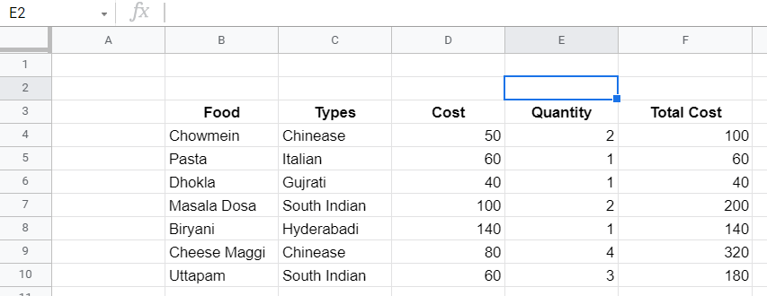
Reference Table: The following table will be used as a reference table for all the examples of the INDEX function. First Cell is at B3 (“FOOD”) and the Last Diagonal Cell is at F10 (“180”).
Examples: Below are some examples of Index functions.
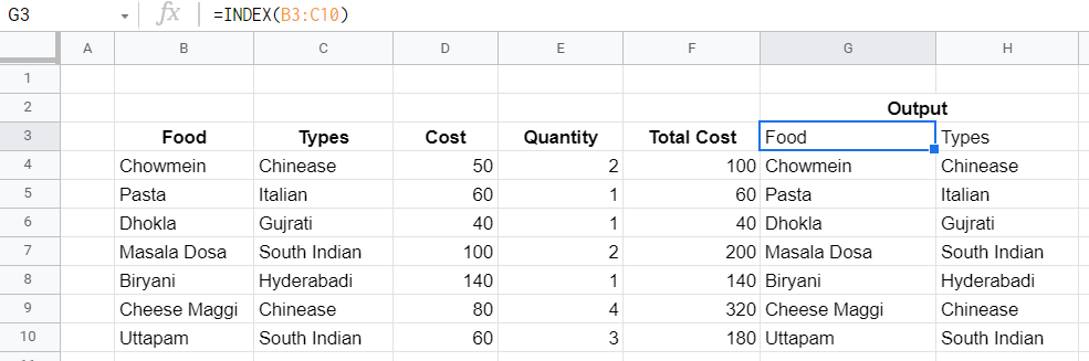
Case 1: No Rows and Columns are mentioned.
Input Command: =INDEX(B3:C10)
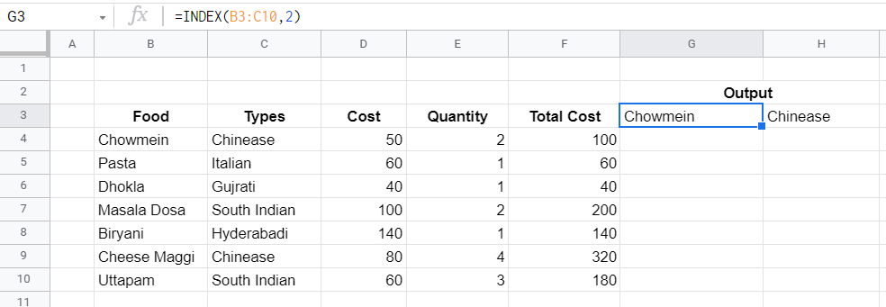
Case 2: Only Rows are Mentioned.
Input Command: =INDEX(B3:C10,2)
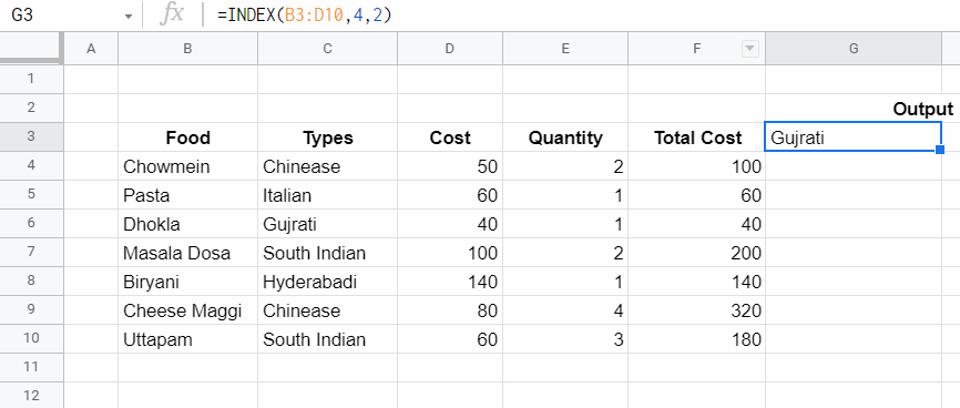
Case 3: Both Rows And Columns are mentioned.
Input Command: =INDEX(B3:D10,4,2)
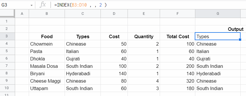
Case 4: Only Columns are mentioned.
Input Command: =INDEX(B3 : D10 , , 2)
Problem With INDEX Function: The problem with the INDEX function is that there is a need to specify rows and columns for the data that we are looking for. Let’s assume we are dealing with a machine learning dataset of 10000 rows and columns then it will be very difficult to search and extract the data that we are looking for. Here comes the concept of Match Function, which will identify rows and columns based on some condition.
MATCH Function
It retrieves the position of an item/value in a range. It is a less refined version of a VLOOKUP or HLOOKUP that only returns the location information and not the actual data. MATCH is not case-sensitive and does not care whether the range is Horizontal or Vertical.
Syntax:
=MATCH(search_key, range, [search_type])
Parameters:
- search_key: The value to search for. For example, 42, “Cats”, or I24.
- range: The one-dimensional array to be searched. It Can Either be a single row or a single column.eg->A1:A10 , A2:D2 etc.
- search_type [optional]: The search method. = 1 (default) finds the largest value less than or equal to search_key when the range is sorted in ascending order.
- = 0 finds the exact value when the range is unsorted.
- = -1 finds the smallest value greater than or equal to search_key when the range is sorted in descending order.
Row number or Column number can be found using the match function and can use it inside the index function so if there is any detail about an item, then all information can be extracted about the item by finding the row/column of the item using match then nesting it into index function.
Reference Table: The following table will be used as a reference table for all the examples of the MATCH function. First Cell is at B3 (“FOOD”) and the Last Diagonal Cell is At F10 (“180”)
Examples: Below are some examples of the MATCH function-
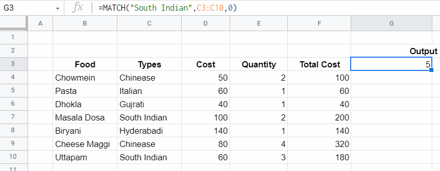
Case 1: Search Type 0, It means Exact Match.
Input Command: =MATCH(“South Indian”,C3:C10,0)
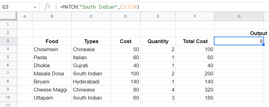
Case 2: Search Type 1 (Default).
Input Command: =MATCH(“South Indian”,C3:C10)
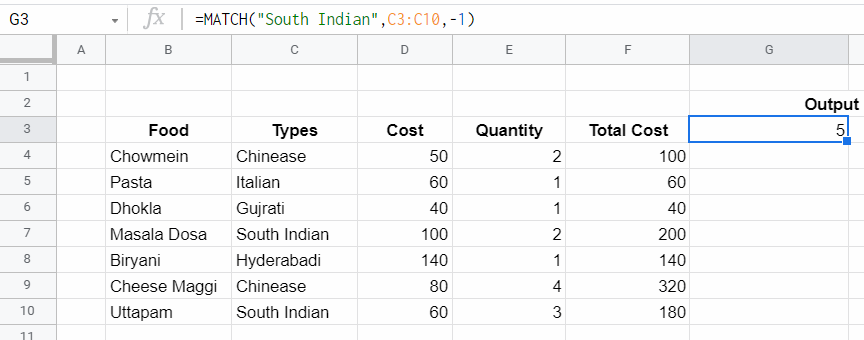
Case 3: Search Type -1.
Input Command: =MATCH(“South Indian”,C3:C10,-1)
INDEX-MATCH Together
In the previous examples, the static values of rows and columns were provided in the INDEX function Let’s assume there is no prior knowledge about the rows and column position then rows and columns position can be provided using the MATCH function. This Is a dynamic way to search and extract value.
Syntax:
=INDEX(Reference Table , [Match(SearchKey,Range,Type)/StaticRowPosition],
                         [Match(SearchKey,Range,Type)/StaticColumnPosition])
Reference Table: The following reference table will be used. First Cell is at B3 (“FOOD”) and the Last Diagonal Cell is At F10 (“180”)
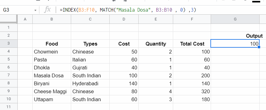
Example: Let’s say the task is to find the cost of Masala Dosa. It is known that column 3 represents the cost of items, but the row position of Masala Dosa is not known. The problem can be divided into two steps-
Step 1: Find the position of Masala Dosa by using the formula:
=MATCH("Masala Dosa",B3:B10,0)
Here B3:B10 represents Column “Food” and 0 means Exact Match. It will return the row number of Masala Dosa.
Step 2: Find the cost of Masala Dosa. Use the INDEX Function to find the cost of Masala Dosa. By substituting the above MATCH function query inside the INDEX function at the place where the exact position of Masala Dosa is required, and the column number of cost is 3 which is already known.
=INDEX(B3:F10, MATCH("Masala Dosa", B3:B10 , 0) ,3)
Two Ways Lookup With INDEX-MATCH Together
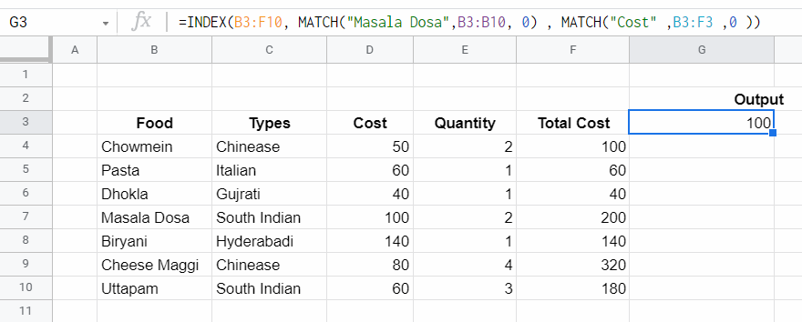
In the previous example, the column position Of the “Cost” attribute was hardcoded. So, It was not fully dynamic.
Case 1: Let’s assume there is no knowledge about the column number of Cost also, then it can be obtained using the formula:
=MATCH("Cost",B3:F3,0)
Here B3:F3 represents Header Column.
Case 2: When row, as well as column value, are provided via MATCH function (without giving static value) then it is called Two-Way Lookup. It can be achieved using the formula:
=INDEX(B3:F10, MATCH("Masala Dosa",B3:B10, 0) , MATCH("Cost" ,B3:F3 ,0))
Left Lookup
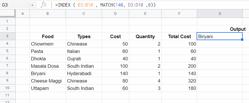
One of the key advantages of INDEX and MATCH over the VLOOKUP function is the ability to perform a “left lookup”. It means it is possible to extract the row position of an item from using any attribute at right and the value of another attribute in left can be extracted.
For Example, Let’s say buy food whose cost should be 140 Rs. Indirectly we are saying buy “Biryani”. In this example, the cost Rs 140/- is known, there is a need to extract the “Food”. Since the Cost column is placed to the right of the Food column. If VLOOKUP is applied it will not be able to search the left side of the Cost column. That is why using VLOOKUP it is not possible to get Food Name.
To overcome this disadvantage INDEX-MATCH function Left lookup can be used.
Step 1: First extract row position of Cost 140 Rs using the formula:
=MATCH(140, D3:D10,0)
Here D3: D10 represents the Cost column where the search for the Cost 140 Rs row number is being done.
Step 2: After getting the row number, the next step is to use the INDEX Function to extract Food Name using the formula:
=INDEX(B3:B10, MATCH(140, D3:D10,0))
Here B3:B10 represents Food Column and 140 is the Cost of the food item.
Case Sensitive Lookup
By itself, the MATCH function is not case-sensitive. This means if there is a Food Name “DHOKLA” and the MATCH function is used with the following search word:
- “Dhokla”
- “dhokla”
- “DhOkLA”
All will return the row position of DHOKLA. However, the EXACT function can be used with INDEX and MATCH to perform a lookup that respects upper and lower case.
Exact Function: The Excel EXACT function compares two text strings, taking into account upper and lower case characters, and returns TRUE if they are the same, and FALSE if not. EXACT is case-sensitive.
Examples:
- EXACT(“DHOKLA”,”DHOKLA”): This will return True.
- EXACT(“DHOKLA”,”Dhokla”): This will return False.
- EXACT(“DHOKLA”,”dhokla”): This will return False.
- EXACT(“DHOKLA”,”DhOkLA”): This will return False.
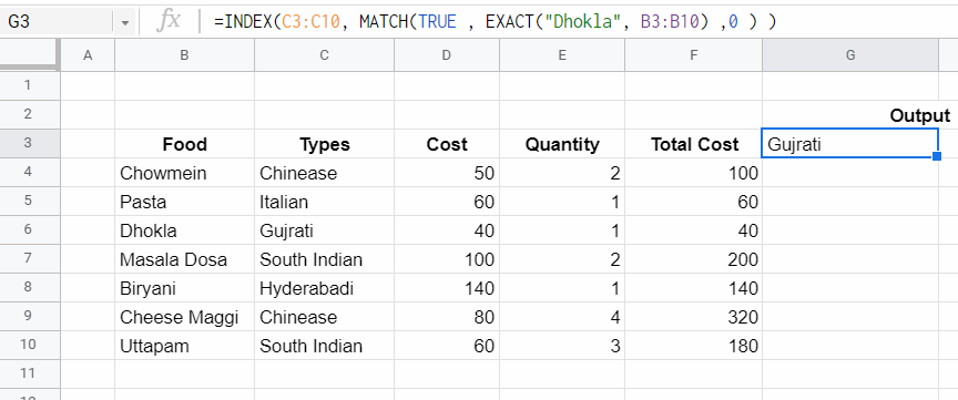
Example: Let say the task is to search for the Type Of Food “Dhokla” but in Case-Sensitive Way. This can be done using the formula-
=INDEX(C3:C10, MATCH(TRUE , EXACT("Dhokla", B3:B10) ,0))
Here the EXACT function will return True if the value in Column B3:B10 matches with “Dhokla” with the same case, else it will return False. Now MATCH function will apply in Column B3:B10 and search for a row with the Exact value TRUE. After that INDEX Function will retrieve the value of Column C3:C10 (Food Type Column) at the row returned by the MATCH function.
Multiple Criteria Lookup
One of the trickiest problems in Excel is a lookup based on multiple criteria. In other words, a lookup that matches on more than one column at the same time. In the example below, the INDEX and MATCH function and boolean logic are used to match on 3 columns-
- Food.
- Cost.
- Quantity.
To extract total cost.
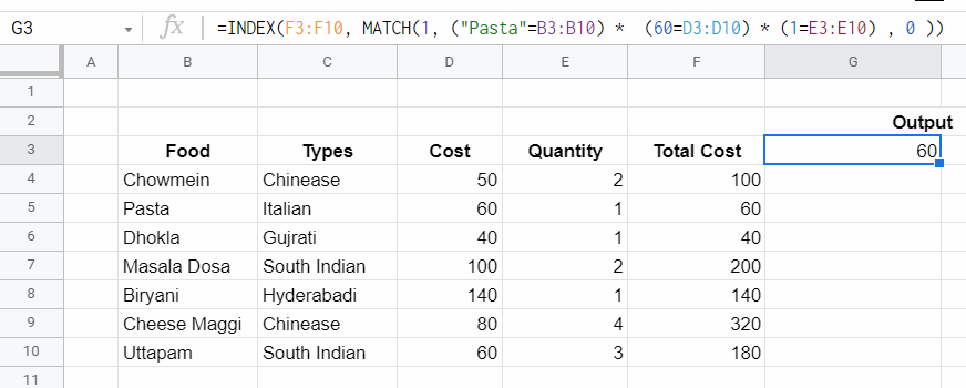
Example: Let’s say the task is to calculate the total cost of Pasta where
- Food: Pasta.
- Cost: 60.
- Quantity: 1.
So in this example, there are three criteria to perform a Match. Below are the steps for the search based on multiple criteria-
Step 1: First match Food Column (B3:B10) with Pasta using the formula:
"PASTA" = B3:B10
This will convert B3:B10 (Food Column) values as Boolean. That Is True where Food is Pasta else False.
Step 2: After that, match Cost criteria in the following manner:
60 = D3:D10
This will replace D3:D10 (Cost Column) values as Boolean. That is True where Cost=60 else False.
Step 3: Next step is to match the third criteria that are Quantity = 1 in the following manner:
1 = E3:E10
This will replace E3:E10 Column (Quantity Column) as True where Quantity = 1 else it will be False.
Step 4: Multiply the result of the first, second, and third criteria. This will be the intersection of all conditions and convert Boolean True / False as 1/0.
Step 5: Now the result will be a Column with 0 And 1. Here use the MATCH Function to find the row number of columns that contain 1. Because if a column is having the value 1, then it means it satisfies all three criteria.
Step 6: After getting the row number use the INDEX function to get the total cost of that row.
=INDEX(F3:F10, MATCH(1, ("Pasta"=B3:B10) * (60=D3:D10) * (1=E3:E10) , 0 ))
Here F3:F10 represents the Total Cost Column.
In this article, we will learn how to Lookup & SUM values with INDEX and MATCH function in Excel.
For the formula to understand first we need to revise a little about the three functions
- SUM
- INDEX
- MATCH
SUM function adds all the numbers in a range of cells and returns the sum of these values.
INDEX function returns the value at a given index in an array.
MATCH function returns the index of the first appearance of the value in an array ( single dimension array ).
Now we will make a formula using the above functions. Match function will return the index of the lookup value in the header field. The index number will now be fed to the INDEX function to get the values under the lookup value.
Then the SUM function will return the sum from the found values.
Use the Formula:
= SUM ( INDEX ( data , 0, MATCH ( lookup_value, headers, 0)))
The above statements can be complicated to understand. So let’s understand this by using the formula in an example
Here we have a list of marks of students and we need to find the total marks for a specific person (Gary) as shown in the snapshot below.
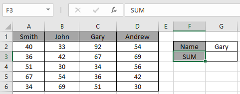
Use the formula in the C2 cell:
= SUM ( INDEX ( A2:D6 , 0 , MATCH ( G2 , A1:D1 , 0 )))
Explanation:
- The MATCH function matches the first value with the header array and returns its position 3 as a number.
- The INDEX function takes the number as the column index for the data and returns the array { 92 ; 67 ; 34 ; 36 ; 51 } to the argument of the SUM function
- The SUM function takes the array and returns the SUM in the cell.
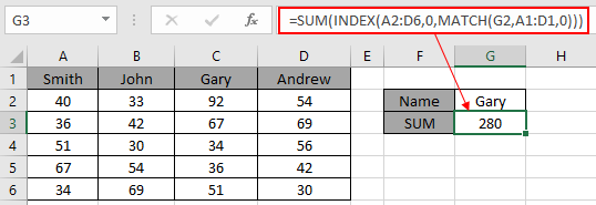
Here values to the function is given as cell reference.
As you can see in the above snapshot, we got the SUM of the marks of student Gary. And it proves the formula works fine and for doubts see the below notes for understanding.
Notes:
- The function returns the #NA error if the lookup array argument to the MATCH function is 2 — D array which is the header field of the data..
- The function matches exact value as the match type argument to the MATCH function is 0.
- The lookup value can be given as cell reference or directly using quote symbol («).
- The SUM function ignores the text values in the array received from the INDEX function.
Hope you understood how to use the LOOKUP function in Excel. Explore more articles on Excel lookup value here. Please feel free to state your queries below in the comment box. We will certainly help you.
Related Articles
Use INDEX and MATCH to Lookup Value
SUM range with INDEX in Excel
How to use the SUM function in Excel
How to use the INDEX function in Excel
How to use the MATCH function in Excel
How to use LOOKUP function in Excel
How to use the VLOOKUP function in Excel
How to use the HLOOKUP function in Excel
Popular Articles
Edit a dropdown list
If with conditional formatting
If with wildcards
Vlookup by date