
This article explains in simple terms how to use INDEX and MATCH together to perform lookups. It takes a step-by-step approach, first explaining INDEX, then MATCH, then showing you how to combine the two functions together to create a dynamic two-way lookup. There are more advanced examples further down the page.
INDEX function | MATCH function | INDEX and MATCH | 2-way lookup | Left lookup | Case-sensitive | Closest match | Multiple criteria | More examples
The INDEX Function
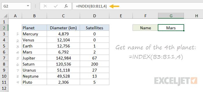
The INDEX function in Excel is fantastically flexible and powerful, and you’ll find it in a huge number of Excel formulas, especially advanced formulas. But what does INDEX actually do? In a nutshell, INDEX retrieves the value at a given location in a range. For example, let’s say you have a table of planets in our solar system (see below), and you want to get the name of the 4th planet, Mars, with a formula. You can use INDEX like this:
=INDEX(B3:B11,4)

INDEX returns the value in the 4th row of the range.
Video: How to look things up with INDEX
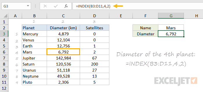
What if you want to get the diameter of Mars with INDEX? In that case, we can supply both a row number and a column number, and provide a larger range. The INDEX formula below uses the full range of data in B3:D11, with a row number of 4 and column number of 2:
=INDEX(B3:D11,4,2)

INDEX retrieves the value at row 4, column 2.
To summarize, INDEX gets a value at a given location in a range of cells based on numeric position. When the range is one-dimensional, you only need to supply a row number. When the range is two-dimensional, you’ll need to supply both the row and column number.
At this point, you may be thinking «So what? How often do you actually know the position of something in a spreadsheet?»
Exactly right. We need a way to locate the position of things we’re looking for.
Enter the MATCH function.
The MATCH function
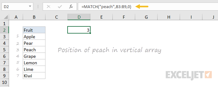
The MATCH function is designed for one purpose: find the position of an item in a range. For example, we can use MATCH to get the position of the word «peach» in this list of fruits like this:
=MATCH("peach",B3:B9,0)

MATCH returns 3, since «Peach» is the 3rd item. MATCH is not case-sensitive.
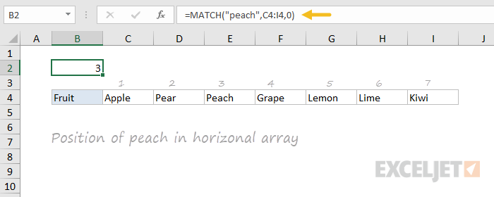
MATCH doesn’t care if a range is horizontal or vertical, as you can see below:
=MATCH("peach",C4:I4,0)

Same result with a horizontal range, MATCH returns 3.
Video: How to use MATCH for exact matches
Important: The last argument in the MATCH function is match_type. Match_type is important and controls whether matching is exact or approximate. In many cases you will want to use zero (0) to force exact match behavior. Match_type defaults to 1, which means approximate match, so it’s important to provide a value. See the MATCH page for more details.
INDEX and MATCH together
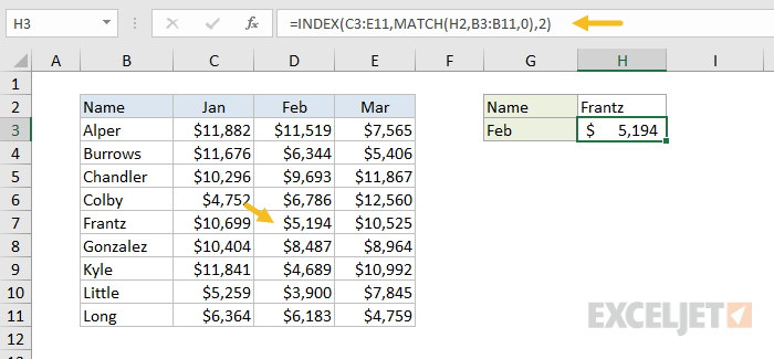
Now that we’ve covered the basics of INDEX and MATCH, how do we combine the two functions in a single formula? Consider the data below, a table showing a list of salespeople and monthly sales numbers for three months: January, February, and March.

Let’s say we want to write a formula that returns the sales number for February for a given salesperson. From the discussion above, we know we can give INDEX a row and column number to retrieve a value. For example, to return the February sales number for Frantz, we provide the range C3:E11 with a row 5 and column 2:
=INDEX(C3:E11,5,2) // returns $5194
But we obviously don’t want to hardcode numbers. Instead, we want a dynamic lookup.
How will we do that? The MATCH function of course. MATCH will work perfectly for finding the positions we need. Working one step at a time, let’s leave the column hardcoded as 2 and make the row number dynamic. Here’s the revised formula, with the MATCH function nested inside INDEX in place of 5:
=INDEX(C3:E11,MATCH("Frantz",B3:B11,0),2)
Taking things one step further, we’ll use the value from H2 in MATCH:
=INDEX(C3:E11,MATCH(H2,B3:B11,0),2)

MATCH finds «Frantz» and returns 5 to INDEX for row.
To summarize:
- INDEX needs numeric positions.
- MATCH finds those positions.
- MATCH is nested inside INDEX.
Let’s now tackle the column number.
Two-way lookup with INDEX and MATCH
Above, we used the MATCH function to find the row number dynamically, but hardcoded the column number. How can we make the formula fully dynamic, so we can return sales for any given salesperson in any given month? The trick is to use MATCH twice – once to get a row position, and once to get a column position.
From the examples above, we know MATCH works fine with both horizontal and vertical arrays. That means we can easily find the position of a given month with MATCH. For example, this formula returns the position of March, which is 3:
=MATCH("Mar",C2:E2,0) // returns 3
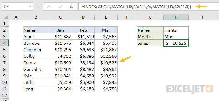
But of course we don’t want to hardcode any values, so let’s update the worksheet to allow the input of a month name, and use MATCH to find the column number we need. The screen below shows the result:

A fully dynamic, two-way lookup with INDEX and MATCH.
=INDEX(C3:E11,MATCH(H2,B3:B11,0),MATCH(H3,C2:E2,0))
The first MATCH formula returns 5 to INDEX as the row number, the second MATCH formula returns 3 to INDEX as the column number. Once MATCH runs, the formula simplifies to:
=INDEX(C3:E11,5,3)
and INDEX correctly returns $10,525, the sales number for Frantz in March.
Note: you could use Data Validation to create dropdown menus to select salesperson and month.
Video: How to do a two-way lookup with INDEX and MATCH
Video: How to debug a formula with F9 (to see MATCH return values)
Left lookup
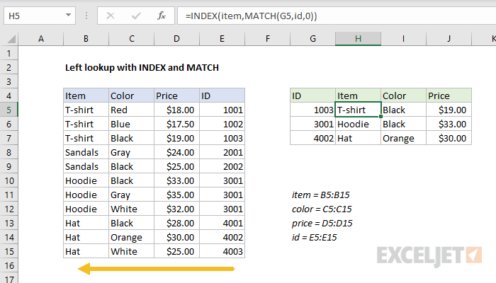
One of the key advantages of INDEX and MATCH over the VLOOKUP function is the ability to perform a «left lookup». Simply put, this just means a lookup where the ID column is to the right of the values you want to retrieve, as seen in the example below:

Read a detailed explanation here.
Case-sensitive lookup
By itself, the MATCH function is not case-sensitive. However, you use the EXACT function with INDEX and MATCH to perform a lookup that respects upper and lower case, as shown below:

Read a detailed explanation here.
Note: this is an array formula and must be entered with control + shift + enter, except in Excel 365.
Closest match
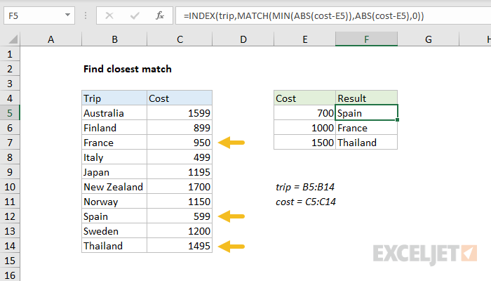
Another example that shows off the flexibility of INDEX and MATCH is the problem of finding the closest match. In the example below, we use the MIN function together with the ABS function to create a lookup value and a lookup array inside the MATCH function. Essentially, we use MATCH to find the smallest difference. Then we use INDEX to retrieve the associated trip from column B.

Read a detailed explanation here.
Note: this is an array formula and must be entered with control + shift + enter, except in Excel 365.
Multiple criteria lookup
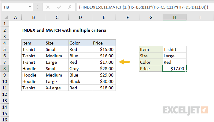
One of the trickiest problems in Excel is a lookup based on multiple criteria. In other words, a lookup that matches on more than one column at the same time. In the example below, we are using INDEX and MATCH and boolean logic to match on 3 columns: Item, Color, and Size:

Read a detailed explanation here. You can use this same approach with XLOOKUP.
Note: this is an array formula and must be entered with control + shift + enter, except in Excel 365.
More examples of INDEX + MATCH
Here are some more basic examples of INDEX and MATCH in action, each with a detailed explanation:
- Basic INDEX and MATCH exact (features Toy Story)
- Basic INDEX and MATCH approximate (grades)
- Two-way lookup with INDEX and MATCH (approximate match)
Содержание
- Look up values with VLOOKUP, INDEX, or MATCH
- Using INDEX and MATCH instead of VLOOKUP
- Give it a try
- VLOOKUP Example at work
- INDEX and MATCH with multiple criteria
- Related functions
- Summary
- Generic formula
- Explanation
- Array visualization
- Non-array version
- MATCH
- Syntax
- Example
- How to use INDEX and MATCH
- Summary
- The INDEX Function
- The MATCH function
- INDEX and MATCH together
- Two-way lookup with INDEX and MATCH
- Left lookup
- Case-sensitive lookup
- Closest match
- Multiple criteria lookup
- More examples of INDEX + MATCH
Look up values with VLOOKUP, INDEX, or MATCH
Tip: Try using the new XLOOKUP and XMATCH functions, improved versions of the functions described in this article. These new functions work in any direction and return exact matches by default, making them easier and more convenient to use than their predecessors.
Suppose that you have a list of office location numbers, and you need to know which employees are in each office. The spreadsheet is huge, so you might think it is challenging task. It’s actually quite easy to do with a lookup function.
The VLOOKUP and HLOOKUP functions, together with INDEX and MATCH, are some of the most useful functions in Excel.
Note: The Lookup Wizard feature is no longer available in Excel.
Here’s an example of how to use VLOOKUP.
In this example, B2 is the first argument—an element of data that the function needs to work. For VLOOKUP, this first argument is the value that you want to find. This argument can be a cell reference, or a fixed value such as «smith» or 21,000. The second argument is the range of cells, C2-:E7, in which to search for the value you want to find. The third argument is the column in that range of cells that contains the value that you seek.
The fourth argument is optional. Enter either TRUE or FALSE. If you enter TRUE, or leave the argument blank, the function returns an approximate match of the value you specify in the first argument. If you enter FALSE, the function will match the value provide by the first argument. In other words, leaving the fourth argument blank—or entering TRUE—gives you more flexibility.
This example shows you how the function works. When you enter a value in cell B2 (the first argument), VLOOKUP searches the cells in the range C2:E7 (2nd argument) and returns the closest approximate match from the third column in the range, column E (3rd argument).
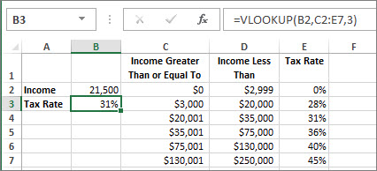
The fourth argument is empty, so the function returns an approximate match. If it didn’t, you’d have to enter one of the values in columns C or D to get a result at all.
When you’re comfortable with VLOOKUP, the HLOOKUP function is equally easy to use. You enter the same arguments, but it searches in rows instead of columns.
Using INDEX and MATCH instead of VLOOKUP
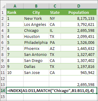
There are certain limitations with using VLOOKUP—the VLOOKUP function can only look up a value from left to right. This means that the column containing the value you look up should always be located to the left of the column containing the return value. Now if your spreadsheet isn’t built this way, then do not use VLOOKUP. Use the combination of INDEX and MATCH functions instead.
This example shows a small list where the value we want to search on, Chicago, isn’t in the leftmost column. So, we can’t use VLOOKUP. Instead, we’ll use the MATCH function to find Chicago in the range B1:B11. It’s found in row 4. Then, INDEX uses that value as the lookup argument, and finds the population for Chicago in the 4th column (column D). The formula used is shown in cell A14.
For more examples of using INDEX and MATCH instead of VLOOKUP, see the article https://www.mrexcel.com/excel-tips/excel-vlookup-index-match/ by Bill Jelen, Microsoft MVP.
Give it a try
If you want to experiment with lookup functions before you try them out with your own data, here’s some sample data.
VLOOKUP Example at work
Copy the following data into a blank spreadsheet.
Tip: Before you paste the data into Excel, set the column widths for columns A through C to 250 pixels, and click Wrap Text ( Home tab, Alignment group).
Источник
INDEX and MATCH with multiple criteria

Summary
To lookup values with INDEX and MATCH, using multiple criteria, you can use an array formula. In the example shown, the formula in H8 is:
The result is $17.00, the Price of a Large Red T-shirt. This is an array formula and must be entered with with Control + Shift + Enter in Legacy Excel.
Note: In the current version of Excel, you can use the same approach with the XLOOKUP function.
Generic formula
Explanation
This is a more advanced formula. For basics, see How to use INDEX and MATCH.
Normally, an INDEX MATCH formula is configured with MATCH set to look through a one-column range and provide a match based on given criteria. Without concatenating values in a helper column, or in the formula itself, there’s no way to supply more than one criteria.
This formula works around this limitation by using boolean logic to create an array of ones and zeros to represent rows matching all 3 criteria, then using MATCH to match the first 1 found. The temporary array of ones and zeros is generated with this snippet:
Here we compare the item in H5 against all items, the size in H6 against all sizes, and the color in H7 against all colors. The initial result is three arrays of TRUE/FALSE results like this:
Tip: use F9 to see these results. Just select an expression in the formula bar, and press F9.
The math operation (multiplication) transforms the TRUE FALSE values to 1s and 0s:
After multiplication, we have a single array like this:
which is fed into the MATCH function as the lookup array, with a lookup value of 1:
At this point, the formula is a standard INDEX MATCH formula. The MATCH function returns 3 to INDEX:
and INDEX returns a final result of $17.00.
Array visualization
The arrays explained above can be difficult to visualize. The image below shows the basic idea. Columns B, C, and D correspond to the data in the example. Column F is created by the multiplying the three columns together. It is the array handed off to MATCH.

Non-array version
It is possible to add another INDEX to this formula, avoiding the need to enter as an array formula with control + shift + enter:
The INDEX function can handle arrays natively, so the second INDEX is added only to «catch» the array created with the boolean logic operation and return the same array again to MATCH. To do this, INDEX is configured with zero rows and one column. The zero row trick causes INDEX to return column 1 from the array (which is already one column anyway).
Why would you want the non-array version? Sometimes, people forget to enter an array formula with control + shift + enter, and the formula returns an incorrect result. So, a non-array formula is more «bulletproof». However, the tradeoff is a more complex formula.
Note: In Excel 365, it is not necessary to enter array formulas in a special way.
Источник
MATCH
Tip: Try using the new XMATCH function, an improved version of MATCH that works in any direction and returns exact matches by default, making it easier and more convenient to use than its predecessor.
The MATCH function searches for a specified item in a range of cells, and then returns the relative position of that item in the range. For example, if the range A1:A3 contains the values 5, 25, and 38, then the formula =MATCH(25,A1:A3,0) returns the number 2, because 25 is the second item in the range.

Tip: Use MATCH instead of one of the LOOKUP functions when you need the position of an item in a range instead of the item itself. For example, you might use the MATCH function to provide a value for the row_num argument of the INDEX function.
Syntax
MATCH(lookup_value, lookup_array, [match_type])
The MATCH function syntax has the following arguments:
lookup_value Required. The value that you want to match in lookup_array. For example, when you look up someone’s number in a telephone book, you are using the person’s name as the lookup value, but the telephone number is the value you want.
The lookup_value argument can be a value (number, text, or logical value) or a cell reference to a number, text, or logical value.
lookup_array Required. The range of cells being searched.
match_type Optional. The number -1, 0, or 1. The match_type argument specifies how Excel matches lookup_value with values in lookup_array. The default value for this argument is 1.
The following table describes how the function finds values based on the setting of the match_type argument.
MATCH finds the largest value that is less than or equal to lookup_value. The values in the lookup_array argument must be placed in ascending order, for example: . -2, -1, 0, 1, 2, . A-Z, FALSE, TRUE.
MATCH finds the first value that is exactly equal to lookup_value. The values in the lookup_array argument can be in any order.
MATCH finds the smallest value that is greater than or equal to lookup_value. The values in the lookup_array argument must be placed in descending order, for example: TRUE, FALSE, Z-A, . 2, 1, 0, -1, -2, . and so on.
MATCH returns the position of the matched value within lookup_array, not the value itself. For example, MATCH(«b», <«a»,»b»,»c «>,0) returns 2, which is the relative position of «b» within the array <«a»,»b»,»c»>.
MATCH does not distinguish between uppercase and lowercase letters when matching text values.
If MATCH is unsuccessful in finding a match, it returns the #N/A error value.
If match_type is 0 and lookup_value is a text string, you can use the wildcard characters — the question mark ( ?) and asterisk ( *) — in the lookup_value argument. A question mark matches any single character; an asterisk matches any sequence of characters. If you want to find an actual question mark or asterisk, type a tilde (
) before the character.
Example
Copy the example data in the following table, and paste it in cell A1 of a new Excel worksheet. For formulas to show results, select them, press F2, and then press Enter. If you need to, you can adjust the column widths to see all the data.
Источник
How to use INDEX and MATCH

Summary
INDEX and MATCH is the most popular tool in Excel for performing more advanced lookups. This is because INDEX and MATCH are incredibly flexible – you can do horizontal and vertical lookups, 2-way lookups, left lookups, case-sensitive lookups, and even lookups based on multiple criteria. If you want to improve your Excel skills, INDEX and MATCH should be on your list. See below for many examples.
This article explains in simple terms how to use INDEX and MATCH together to perform lookups. It takes a step-by-step approach, first explaining INDEX, then MATCH, then showing you how to combine the two functions together to create a dynamic two-way lookup. There are more advanced examples further down the page.
The INDEX Function
The INDEX function in Excel is fantastically flexible and powerful, and you’ll find it in a huge number of Excel formulas, especially advanced formulas. But what does INDEX actually do? In a nutshell, INDEX retrieves the value at a given location in a range. For example, let’s say you have a table of planets in our solar system (see below), and you want to get the name of the 4th planet, Mars, with a formula. You can use INDEX like this:
INDEX returns the value in the 4th row of the range.
What if you want to get the diameter of Mars with INDEX? In that case, we can supply both a row number and a column number, and provide a larger range. The INDEX formula below uses the full range of data in B3:D11, with a row number of 4 and column number of 2:
INDEX retrieves the value at row 4, column 2.
To summarize, INDEX gets a value at a given location in a range of cells based on numeric position. When the range is one-dimensional, you only need to supply a row number. When the range is two-dimensional, you’ll need to supply both the row and column number.
At this point, you may be thinking «So what? How often do you actually know the position of something in a spreadsheet?»
Exactly right. We need a way to locate the position of things we’re looking for.
Enter the MATCH function.
The MATCH function
The MATCH function is designed for one purpose: find the position of an item in a range. For example, we can use MATCH to get the position of the word «peach» in this list of fruits like this:
MATCH returns 3, since «Peach» is the 3rd item. MATCH is not case-sensitive.
MATCH doesn’t care if a range is horizontal or vertical, as you can see below:
Same result with a horizontal range, MATCH returns 3.
Important: The last argument in the MATCH function is match_type. Match_type is important and controls whether matching is exact or approximate. In many cases you will want to use zero (0) to force exact match behavior. Match_type defaults to 1, which means approximate match, so it’s important to provide a value. See the MATCH page for more details.
INDEX and MATCH together
Now that we’ve covered the basics of INDEX and MATCH, how do we combine the two functions in a single formula? Consider the data below, a table showing a list of salespeople and monthly sales numbers for three months: January, February, and March.
Let’s say we want to write a formula that returns the sales number for February for a given salesperson. From the discussion above, we know we can give INDEX a row and column number to retrieve a value. For example, to return the February sales number for Frantz, we provide the range C3:E11 with a row 5 and column 2:
But we obviously don’t want to hardcode numbers. Instead, we want a dynamic lookup.
How will we do that? The MATCH function of course. MATCH will work perfectly for finding the positions we need. Working one step at a time, let’s leave the column hardcoded as 2 and make the row number dynamic. Here’s the revised formula, with the MATCH function nested inside INDEX in place of 5:
Taking things one step further, we’ll use the value from H2 in MATCH:
MATCH finds «Frantz» and returns 5 to INDEX for row.
- INDEX needs numeric positions.
- MATCH finds those positions.
- MATCH is nested inside INDEX.
Let’s now tackle the column number.
Two-way lookup with INDEX and MATCH
Above, we used the MATCH function to find the row number dynamically, but hardcoded the column number. How can we make the formula fully dynamic, so we can return sales for any given salesperson in any given month? The trick is to use MATCH twice – once to get a row position, and once to get a column position.
From the examples above, we know MATCH works fine with both horizontal and vertical arrays. That means we can easily find the position of a given month with MATCH. For example, this formula returns the position of March, which is 3:
But of course we don’t want to hardcode any values, so let’s update the worksheet to allow the input of a month name, and use MATCH to find the column number we need. The screen below shows the result:
A fully dynamic, two-way lookup with INDEX and MATCH.
The first MATCH formula returns 5 to INDEX as the row number, the second MATCH formula returns 3 to INDEX as the column number. Once MATCH runs, the formula simplifies to:
and INDEX correctly returns $10,525, the sales number for Frantz in March.
Note: you could use Data Validation to create dropdown menus to select salesperson and month.
Video: How to debug a formula with F9 (to see MATCH return values)
Left lookup
One of the key advantages of INDEX and MATCH over the VLOOKUP function is the ability to perform a «left lookup». Simply put, this just means a lookup where the ID column is to the right of the values you want to retrieve, as seen in the example below:
Case-sensitive lookup
By itself, the MATCH function is not case-sensitive. However, you use the EXACT function with INDEX and MATCH to perform a lookup that respects upper and lower case, as shown below:
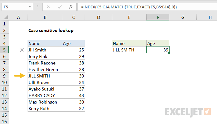
Note: this is an array formula and must be entered with control + shift + enter, except in Excel 365.
Closest match
Another example that shows off the flexibility of INDEX and MATCH is the problem of finding the closest match. In the example below, we use the MIN function together with the ABS function to create a lookup value and a lookup array inside the MATCH function. Essentially, we use MATCH to find the smallest difference. Then we use INDEX to retrieve the associated trip from column B.
Note: this is an array formula and must be entered with control + shift + enter, except in Excel 365.
Multiple criteria lookup
One of the trickiest problems in Excel is a lookup based on multiple criteria. In other words, a lookup that matches on more than one column at the same time. In the example below, we are using INDEX and MATCH and boolean logic to match on 3 columns: Item, Color, and Size:
Note: this is an array formula and must be entered with control + shift + enter, except in Excel 365.
More examples of INDEX + MATCH
Here are some more basic examples of INDEX and MATCH in action, each with a detailed explanation:
Источник
MATCH function
Tip: Try using the new XMATCH function, an improved version of MATCH that works in any direction and returns exact matches by default, making it easier and more convenient to use than its predecessor.
The MATCH function searches for a specified item in a range of cells, and then returns the relative position of that item in the range. For example, if the range A1:A3 contains the values 5, 25, and 38, then the formula =MATCH(25,A1:A3,0) returns the number 2, because 25 is the second item in the range.
Tip: Use MATCH instead of one of the LOOKUP functions when you need the position of an item in a range instead of the item itself. For example, you might use the MATCH function to provide a value for the row_num argument of the INDEX function.
Syntax
MATCH(lookup_value, lookup_array, [match_type])
The MATCH function syntax has the following arguments:
-
lookup_value Required. The value that you want to match in lookup_array. For example, when you look up someone’s number in a telephone book, you are using the person’s name as the lookup value, but the telephone number is the value you want.
The lookup_value argument can be a value (number, text, or logical value) or a cell reference to a number, text, or logical value.
-
lookup_array Required. The range of cells being searched.
-
match_type Optional. The number -1, 0, or 1. The match_type argument specifies how Excel matches lookup_value with values in lookup_array. The default value for this argument is 1.
The following table describes how the function finds values based on the setting of the match_type argument.
|
Match_type |
Behavior |
|
1 or omitted |
MATCH finds the largest value that is less than or equal to lookup_value. The values in the lookup_array argument must be placed in ascending order, for example: …-2, -1, 0, 1, 2, …, A-Z, FALSE, TRUE. |
|
0 |
MATCH finds the first value that is exactly equal to lookup_value. The values in the lookup_array argument can be in any order. |
|
-1 |
MATCH finds the smallest value that is greater than or equal tolookup_value. The values in the lookup_array argument must be placed in descending order, for example: TRUE, FALSE, Z-A, …2, 1, 0, -1, -2, …, and so on. |
-
MATCH returns the position of the matched value within lookup_array, not the value itself. For example, MATCH(«b»,{«a»,»b»,»c«},0) returns 2, which is the relative position of «b» within the array {«a»,»b»,»c»}.
-
MATCH does not distinguish between uppercase and lowercase letters when matching text values.
-
If MATCH is unsuccessful in finding a match, it returns the #N/A error value.
-
If match_type is 0 and lookup_value is a text string, you can use the wildcard characters — the question mark (?) and asterisk (*) — in the lookup_value argument. A question mark matches any single character; an asterisk matches any sequence of characters. If you want to find an actual question mark or asterisk, type a tilde (~) before the character.
Example
Copy the example data in the following table, and paste it in cell A1 of a new Excel worksheet. For formulas to show results, select them, press F2, and then press Enter. If you need to, you can adjust the column widths to see all the data.
|
Product |
Count |
|
|
Bananas |
25 |
|
|
Oranges |
38 |
|
|
Apples |
40 |
|
|
Pears |
41 |
|
|
Formula |
Description |
Result |
|
=MATCH(39,B2:B5,1) |
Because there is not an exact match, the position of the next lowest value (38) in the range B2:B5 is returned. |
2 |
|
=MATCH(41,B2:B5,0) |
The position of the value 41 in the range B2:B5. |
4 |
|
=MATCH(40,B2:B5,-1) |
Returns an error because the values in the range B2:B5 are not in descending order. |
#N/A |
Need more help?
Want more options?
Explore subscription benefits, browse training courses, learn how to secure your device, and more.
Communities help you ask and answer questions, give feedback, and hear from experts with rich knowledge.
In this article, we will learn how to Lookup & SUM values with INDEX and MATCH function in Excel.
For the formula to understand first we need to revise a little about the three functions
- SUM
- INDEX
- MATCH
SUM function adds all the numbers in a range of cells and returns the sum of these values.
INDEX function returns the value at a given index in an array.
MATCH function returns the index of the first appearance of the value in an array ( single dimension array ).
Now we will make a formula using the above functions. Match function will return the index of the lookup value in the header field. The index number will now be fed to the INDEX function to get the values under the lookup value.
Then the SUM function will return the sum from the found values.
Use the Formula:
= SUM ( INDEX ( data , 0, MATCH ( lookup_value, headers, 0)))
The above statements can be complicated to understand. So let’s understand this by using the formula in an example
Here we have a list of marks of students and we need to find the total marks for a specific person (Gary) as shown in the snapshot below.
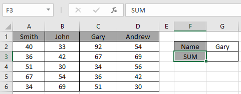
Use the formula in the C2 cell:
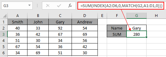
= SUM ( INDEX ( A2:D6 , 0 , MATCH ( G2 , A1:D1 , 0 )))
Explanation:
- The MATCH function matches the first value with the header array and returns its position 3 as a number.
- The INDEX function takes the number as the column index for the data and returns the array { 92 ; 67 ; 34 ; 36 ; 51 } to the argument of the SUM function
- The SUM function takes the array and returns the SUM in the cell.
Here values to the function is given as cell reference.
As you can see in the above snapshot, we got the SUM of the marks of student Gary. And it proves the formula works fine and for doubts see the below notes for understanding.
Notes:
- The function returns the #NA error if the lookup array argument to the MATCH function is 2 — D array which is the header field of the data..
- The function matches exact value as the match type argument to the MATCH function is 0.
- The lookup value can be given as cell reference or directly using quote symbol («).
- The SUM function ignores the text values in the array received from the INDEX function.
Hope you understood how to use the LOOKUP function in Excel. Explore more articles on Excel lookup value here. Please feel free to state your queries below in the comment box. We will certainly help you.
Related Articles
Use INDEX and MATCH to Lookup Value
SUM range with INDEX in Excel
How to use the SUM function in Excel
How to use the INDEX function in Excel
How to use the MATCH function in Excel
How to use LOOKUP function in Excel
How to use the VLOOKUP function in Excel
How to use the HLOOKUP function in Excel
Popular Articles
Edit a dropdown list
If with conditional formatting
If with wildcards
Vlookup by date
If there is no match, then Match() will return the #N/A error, which will be multiplied with the other Match() result and still return an error. Therefore, this formula will only have a non-error result if BOTH Match formulas return a proper value. That’s not what you want, I assume.
You need a formula or function that does not resolve in an error if there is only one match for the two conditions.
One option is to encase each Match into an Iferror. Anonther option is to use Countif, along the lines of this:
=if(countif(G:G,A2)+countif(G:G,B2),"Present","Absent")
Countif returns 0 if nothing is found or a count of the items found. The zero will equal a FALSE in the IF statement, so if neither Countif finds anything, the FALSE argument of the IF function will fire. Bit if any of the two Countif functions find a match, the result will be a number greater than zero, so the TRUE part of the IF function will fire.
На чтение 2 мин
Функция ПОИСКПОЗ в Excel используют для поиска точной позиции искомого значения в списке или массиве данных.
Содержание
- Что возвращает функция
- Синтаксис
- Аргументы функции
- Дополнительная информация
- Примеры использования функции ПОИСКПОЗ в Excel
Что возвращает функция
Возвращает число, соответствующее позиции искомого значения.
 Больше лайфхаков в нашем Telegram Подписаться
Синтаксис
=MATCH(lookup_value, lookup_array, [match_type]) — английская версия
=ПОИСКПОЗ(искомое_значение;просматриваемый_массив;[тип_сопоставления]) — русская версия
Аргументы функции
- lookup_value (искомое_значение) — значение, с которым вы хотите сопоставить данные из массива или списка данных;
- lookup_array (просматриваемый_массив) — диапазон ячеек в котором вы осуществляете поиск искомых данных;
- [match_type] ([тип_сопоставления]) — (не обязательно) — этот аргумент определяет каким образом, будет осуществлен поиск. Допустимые значения для аргумента: «-1», «0», «1» (подробней читайте ниже).
Дополнительная информация
- Чаще всего функция MATCH используется в сочетании с функцией INDEX (ИНДЕКС);
- Подстановочные знаки могут использоваться в аргументах функции в тех случаях, когда значение поиска — текстовая строка;
- При использовании функции ПОИСКПОЗ регистр букв не учитывается;
- Функция возвращает #N/A ошибку, если искомое значение не найдено;
- Аргумент match_type (тип_сопоставления) определяет каким образом, будет осуществлен поиск:
— Если аргумент match_type (тип_сопоставления) = 0, то это критерий точного соответствия. Он возвращает первую точную позицию соответствия (или ошибку, если совпадения нет);
— Если аргумент match_type (тип_сопоставления) = 1 (по умолчанию), то в таком случае данные должны быть отсортированы в порядке возрастания для этой опции. Функция возвращает наибольшее значение, равное или меньшее значения поиска.
— Если аргумент match_type (тип_сопоставления) = -1, то в таком случае данные должны быть отсортированы в порядке убывания для этой опции. Функция возвращает наименьшее и наибольшее значения поиска.
Примеры использования функции ПОИСКПОЗ в Excel